Article

Daytime Rainy Cloud Detection and Convective Precipitation Delineation Based on a Deep Neural Network Method Using GOES-16 ABI Images

1
NSF Spatiotemporal Innovation Center, George Mason Univ., Fairfax, VA 22030, USA
2
Department of Geography and GeoInformation Science, George Mason Univ., Fairfax, VA 22030, USA
3
Department of Geography, Pennsylvania State University, State College, PA 16801, USA
4
Department of Atmospheric, Oceanic and Earth Sciences, George Mason Univ., Fairfax, VA 22030, USA
5
NASA Center for Climate Simulation, Greenbelt, MD 20771, USA
*
Author to whom correspondence should be addressed.
Remote Sens. 2019, 11(21), 2555; https://doi.org/10.3390/rs11212555
Submission received: 27 September 2019 / Revised: 19 October 2019 / Accepted: 26 October 2019 / Published: 30 October 2019
(This article belongs to the Section Atmospheric Remote Sensing)

Abstract

:
Precipitation, especially convective precipitation, is highly associated with hydrological disasters (e.g., floods and drought) that have negative impacts on agricultural productivity, society, and the environment. To mitigate these negative impacts, it is crucial to monitor the precipitation status in real time. The new Advanced Baseline Imager (ABI) onboard the GOES-16 satellite provides such a precipitation product in higher spatiotemporal and spectral resolutions, especially during the daytime. This research proposes a deep neural network (DNN) method to classify rainy and non-rainy clouds based on the brightness temperature differences (BTDs) and reflectances (Ref) derived from ABI. Convective and stratiform rain clouds are also separated using similar spectral parameters expressing the characteristics of cloud properties. The precipitation events used for training and validation are obtained from the IMERG V05B data, covering the southeastern coast of the U.S. during the 2018 rainy season. The performance of the proposed method is compared with traditional machine learning methods, including support vector machines (SVMs) and random forest (RF). For rainy area detection, the DNN method outperformed the other methods, with a critical success index (CSI) of 0.71 and a probability of detection (POD) of 0.86. For convective precipitation delineation, the DNN models also show a better performance, with a CSI of 0.58 and POD of 0.72. This automatic cloud classification system could be deployed for extreme rainfall event detection, real-time forecasting, and decision-making support in rainfall-related disasters.

Graphical Abstract

1. Introduction

Precipitation is one of the most significant contributing factors to destructive natural disasters globally, including hurricanes, floods, and droughts. Convective precipitation with abnormal activities may lead to severe urban floods [1], landslides [2], and flash floods [3], which cause devastating short-term and long-term impacts on people, economies, infrastructure, and ecosystems. To mitigate these negative impacts, precipitation detection and convective precipitation detection are essential in extreme precipitation monitoring, forecasting, and early warning systems. Recently, the increasing availability of high spatiotemporal resolution datasets is contributing to the real-time detection and monitoring of precipitation events in a limited fashion for various domains, including environmental science [4], climate change [5], the economy [6], and society [7]. For example, rain gauge data provide accurate measurements of precipitation rate [8], while their discrete distributions are limited in both space and time. Passive microwave (PMW) remote sensing is a widely-used technique to retrieve precipitation rate but is restricted in spatial-temporal resolutions and time effectiveness, limiting its resolution in fine-scale disaster warning and real-time precipitation monitoring. In contrast, optical sensors onboard geostationary satellites offer higher spatial and temporal resolutions [9]. The available spectral information and resolutions for extracting the properties of rainy clouds (e.g., cloud top height, cloud top temperature, cloud phase, cloud water path [10]) are becoming increasingly accurate. Infrared (IR) data are more widely used in authoritative precipitation products including the Tropical Rainfall Measuring Mission (TRMM) 3B42 [11], Integrated Multi-Satellite Retrievals for Global Precipitation Measurement (IMERG) [12], and Climate Prediction Center Morphing Technique (CMORPH) global precipitation analyses [13]. Given the advantages of optical sensor data, this paper focuses on rainy cloud detection and convective precipitation delineation using images of IR and the visible spectrum.
Rainy cloud detection is more complicated than merely extracting the cloud area, especially when different types of rainy clouds overlap. There are two major types of clouds that produce precipitation - nimbostratus and cumulonimbus clouds [14,15]. A nimbostratus cloud has a low altitude and is dark, textureless, and thick when observed from the Earth’s surface in the daytime. This kind of cloud typically produces light or moderate precipitation of longer duration (i.e., stratiform precipitation). Cumulonimbus clouds form when the atmosphere is unstable enough to allow for significant vertical growth of a cumulus cloud, [16]. This type of cloud also has typically low base heights of about 300 meters but with tops reaching 15 km.
Cumulonimbus clouds produce more substantial and intense precipitation than nimbostratus clouds, usually along with thunder and lightning due to the collisions between charged water droplets, graupel (ice–water mix), and ice crystal particles. Different kinds of rainy clouds have signature characteristics in both reflectance and brightness temperature (BT). Rainy cloud types are identified using properties that reflect these features, such as cloud height, optical thickness, cloud-top temperature, and particle size. For example, differentiating rainy clouds from non-rainy clouds is achieved using their lower temperature in IR spectrums and unique color and brightness in the visible (VIS) spectrum. Estimating the volume of precipitation is achieved by measuring the cloud’s time period at a specific critical threshold temperature or [17].
To improve the CCD method in estimating convective precipitation, Lazri et al. [18] proposed the cold cloud phase duration (CCPD). Using a thresholding approach, Arai [19] detected rainy clouds with visible and thermal IR imageries of Advanced Very High Resolution Radiometer (AVHRR) data and compared the results with radar data for validation. Tebbi and Haddad [20] trained a support vector machine (SVM) classifier using the brightness temperature difference (BTD) spectral parameters of the Spinning Enhanced Visible and Infrared Imager (SEVIRI) to detect rainy clouds and extract convective clouds in the northern border of Algeria and validated the results using observations from rain gauges. Using SEVIRI data in northern Algeria, Mohia et al. [21] trained a classifier based on the artificial neural multilayer perceptron network (MLP). Improved from AVHRR and SEVIRI, the new generation Advanced Baseline Imager (ABI) was developed with higher spatial, temporal, and spectral resolutions. The ABI provides images with more thermal and spectral bands and visible colors and brightness, resulting in a more sensitive and accurate detection of different kinds of clouds. The high scanning frequency of ABI also allows expedient reactions to precipitation-related disasters, which is essential for the coastlines of the U.S. East Coast study area.
With the advancements in AI and big data techniques, machine and deep learning methods have been developed to investigate climatological phenomena and predict natural disasters [22]. McGovern et al. [23] applied gradient-boosted regression trees (GBRT), RF, and elastic net techniques using physical features of the environment (e.g., condensation level, humidity, updraft speed) to improve the predictability of high-impact weather events (e.g., storm duration, severe wind, severe hail, precipitation classification, forecasting for renewable energy, aviation turbulence). Cloud and precipitation properties are non-linearly related to the information extracted from meteorological data, including satellite images [24]. Meyer et al. [25] compared four machine learning (ML) algorithms (random forests (RFs), neural networks (NNETs), averaged neural networks (AVNNETs), and support vector machines (SVMs)) in precipitation area detection and precipitation rate assessment using SEVIRI data over Germany. They concluded that no single method was better than the others, and modification in spectral parameters was of greater necessity than the choice of ML algorithms.
Although traditional machine learning methods have shown potential in precipitation detection and monitoring, deep learning (DL) approaches are more accurate in processing big data with various features [26], most notably, remote sensing images with better spatiotemporal resolution and more spectral information. To further examine the capability of deep neural networks (DNNs), this paper proposes an automatic rainy cloud detection system based on DNN models and compares the system’s performance with that of traditional machine learning methods (e.g., SVM, RF). With the high spatiotemporal resolution of ABI images, the proposed system has good performance in real-time regional and local precipitation monitoring. Including full coverage of precipitation characteristics of the study area, IMERG is a more accurate assessment of precipitation attributes in contrast to discretely distributed ground observations. This paper also evaluates the system in a hydrological extreme (e.g., hurricane) to provide a meaningful basis and reference for future studies. The remaining part of this paper is organized as follows. Section 2 introduces the study area and the dataset used as training and testing data; Section 3 describes the data processing procedure and the DNN model development; Section 4 validates the proposed method and compares the performance with other methods; Section 5 demonstrates the capability of the proposed method in case studies of normal precipitation events and Hurricane Florence; Section 6 discusses the potential future improvements of the proposed method; Section 7 offers conclusions according to the results of the experiments and use-case analysis.

2. Data and Spectral Parameters

2.1. Study Area

The study focuses on a rectangular area of the U.S. East Coast (32°N to 39°N, 80°W to 75°W) crossing Pennsylvania, Delaware, Maryland, Washington DC, Virginia, and North and South Carolina (Figure 1). The climate of the study area is characterized by cool to cold winters and hot, humid summers. The volume, frequency, and density of precipitation in the study area are significantly higher in all seasons than in other parts of the U.S. [27]. A plethora of training and testing samples for both stratiform and convective precipitation are extractable to build the classification models, making the area suitable for the study of precipitation. A large number of hurricanes and tropical cyclones made landfall in this area in the past century, making the rainy cloud classification system critical for hydrological disasters such as hurricanes.

2.2. GPM-IMERG Precipitation Estimates and Gauge Data

Instead of rain gauge data, which are commonly used in precipitation detection research, IMERG V5B precipitation products are used in this research to distinguish rainy/non-rainy areas and convective/stratiform areas. The IMERG has a spatiotemporal resolution of 0.1° and 30 mins. The precipitation product is generated based on the following five steps. (1) Passive microwave (PMW) estimates are produced and inter-calibrated by the retrieval algorithm. (2) Spatiotemporal interpolations are carried out to obtain adequate sampling. (3) Holes are filled in the PMW constellation using microwave-calibrated IR estimates. (4) Gauge observations are adopted to control bias. (5) Error estimates and product delivery are accomplished [28]. The IMERG is a series of state-of-the-art, high-resolution QPE (quantitative precipitation estimation) products, higher in spatial and temporal resolutions and lower in bias with ground truth compared to the former TRMM series. It is a merged dataset that takes advantage of various global scale PMW and IR constellations and is one of the most accurate and popular precipitation products [29,30]. It has relatively high accuracy in determining rainy areas and convective areas.
Gauge data are not used in this study for the following reasons. (1) Gauge observations are distributed sparsely in our study area, with a density of 0.035 gauges per 100 km2 (122 gauges in the study area of 350,000 km2), and the sparseness of this distribution does not provide enough training and testing samples for the models and is insufficient in reflecting sky conditions. (2) Publicly accessible gauge observations are usually non-uniform in temporal resolution, resulting in the samples being distributed unevenly at different times and introducing bias to the models. For example, some gauge records are in an hourly time step, while others have a time step of 30 or 15 minutes; this feature might not capture short convective precipitation events.

2.3. GOES-16 ABI Data

The Geostationary Operational Environmental Satellite (GOES)-16 is the current operational geostationary satellite operated by the National Oceanic and Atmospheric Administration (NOAA) and National Aeronautics and Space Administration (NASA) and is also known as the GOES-East member of the GOES-West and GOES-East NOAA system. It was launched on 9 November 2016 and has provided data since November 2017. The Advanced Baseline Imager (ABI) instrument onboard GOES-16 provides 16 spectral bands, including two VIS, four near-infrared (NIR), and ten IR channels. Due to the lack of the three VIS and NIR bands during nighttime, this research focuses on rainy cloud detection and convective area delineation in the daytime. Eleven bands are used to calculate the spectral parameters in the detection and delineation procedure (i.e., 2, 3, 6, 8, 10–16). Detailed information regarding the central wavelengths and spatial resolutions for each band are available in Table 1 [31]. The ABI generates an image of the contiguous U.S. (CONUS) every five minutes, and its L1b data used in this study are accurately registered (resampled) to a fixed grid (angle–angle coordinate system) with three different spatial resolutions at a nadir [32] ranging from 0.5 to 1 km and 2 km for different bands. Since it has different spatial and temporal resolutions from that of IMERG, collocating the ABI and IMERG data in both spatiotemporal dimensions is needed (Section 3.1).

2.4. Spectral Parameters

The ability of a particular kind of cloud to produce precipitation and develop heavy rate convective precipitation depends on the altitude of the cloud top and the thickness of the cloud [33]. If a cloud is high enough in altitude, thick enough to carry a large volume of water vapor, and contains ice particles in its upper cloud layers, the chance of producing precipitation increases. As an effective measurement of the potential for precipitation to form in the clouds, the liquid water path (LWP) can be calculated as the measurement of the vertically integrated liquid water content in clouds [34,35,36,37]:
LWP   =   5 9 ρ w τ r e ( h ) ,
where ρ w (g/ m 3 ) is the density of liquid water, τ is the optical thickness, and r e ( h ) is the cloud effective radius determined by the cloud thickness (h). The 2.24 μm channel reflects the size of cloud particles, especially those below the cloud top [38]; therefore, it is used in the calculation of LWP and provides useful information in rainy cloud identification.
To classify different types of sky conditions and clouds according to the precipitation properties, the LWP is reflected by the spectral parameters. Cloud-top temperature (CTT) is a direct indicator of parameters in LWP and reflecting cloud altitude. The CTT is related to the intensity of precipitation from colder cloud tops, which are more likely to produce heavier precipitation [39]. The IR channels of ABI provide CTT information in different spectral ranges. The VIS and NIR bands reflect the unique color and brightness of rainy clouds in the daytime [40]. Effective spectral parameters of the classification system are created and calculated from the combination of these bands from VIS to far IR. Due to the lack of VIS and NIR information in the nighttime, this research focuses on daytime rain cloud monitoring. In total, 15 spectral parameters are selected to optimize the detection accuracy—BT10.35, ΔBT6.19-10.35, ΔBT7.34-12.3, ΔBT6.19-7.34, ΔBT13.3-10.35, ΔBT9.61-13.3, ΔBT8.5-10.35, ΔBT8.5-12.3, BT6.19, ΔBT7.34-8.5, ΔBT7.34-11.2, ΔBT11.2-12.3, and reflectance (Ref) of 3 VIS and NIR bands, Ref0.64, Ref0.865, and Ref2.24. For BT and Ref, the subscript number is the central wavelength of the band, and for BTD (ΔBT), the subscript numbers indicate the central wavelengths (Table 2).
The 10.35 μm channel is an atmospheric window channel providing rich CTT information. It is effective in precipitation estimation, and especially for convective areas [41]. A low temperature in this band indicates a high cloud with a higher probability of producing precipitation and developing into a convective event. The CO2 absorption channel is at 13.3 μm, and CO2 decreases with altitude. Therefore, this channel’s temperature is smaller for lower-level versus higher-level clouds. Since the temperature at 10.35 μm has an inverse relationship with height, ΔBT13.3-10.35 is useful in estimating cloud-top height.
The 6.19 μm and 7.34 μm channels represent water vapor. The differences between their brightness temperatures and those observed in the longwave IR bands (i.e., 10.35 μm, 12.3 μm) represent the summit altitude of the cloud. These BTDs are accurate indicators of whether the cloud level is high enough to become convective areas. At low altitudes, cloud temperature in water vapor channels is lower than that in 10.35 and 12.3 μm bands due to the water vapor absorption. As a result, ΔBT6.19-10.35 and BT7.34-12.3 return negative values for low clouds and slightly negative values for rainy clouds, especially convective clouds. The ΔBT6.19-7.34 is also adopted because it reflects cloud height and thickness, with significantly negative values for mid-level clouds and small negative values for high thick clouds [42]. Additionally, the BT of the upper-level water vapor channel (6.19 μm) is an independent parameter due to its capability to detect rainy and convective clouds.
The information derived from the 11.2 μm channel is similar to that of the 10.35 μm channel, so ΔBT7.34-11.2 reflects the CTT and cloud height. The BTD between 10.35 and 12.3 μm is effective in estimating low-level moisture and cloud particle size [43].
The ΔBT9.61-13.3 is another indicator of cloud top height. The 9.61 and 13.3 μm wavelengths are the ozone and CO2 absorption channels, respectively. The temperature of the 9.61 μm channel is higher for high-altitude clouds because of the warming effect of ozone. Therefore, positive values of ΔBT9.61-13.3 represent high-level clouds, while negative values represent low-level clouds.
The ΔBT8.5-10.35 is used to extract information on the cloud phase and the partitioning of cloud into “water” or “ice” [44] because water versus ice absorption differs in these two channels [45] as witnessed by a positive value for ice clouds and a small negative value for low-level water clouds. Convective precipitation is more related to ice clouds [46].
The ΔBT8.5-12.3 indicates the optical thickness of clouds, returning positive values for high clouds, which are relatively thick with larger particle sizes. Negative values result from low-level water clouds due to the low temperature of water vapor in 8.5 μm. The ΔBT7.34-8.5 also indicates the cloud optical thickness, which is adopted in the precipitation rate retrieval algorithm of ABI [47].
Three additional parameters are selected from the ABI’s VIS and NIR channels to optimize accuracy. Refs of 0.64 μm and 0.865 μm provide cloud brightness. Clouds with higher reflectance in the VIS bands tend to have more water or ice contents, which potentially results in more rainfall and vice versa [48].

3. Methodology and Models

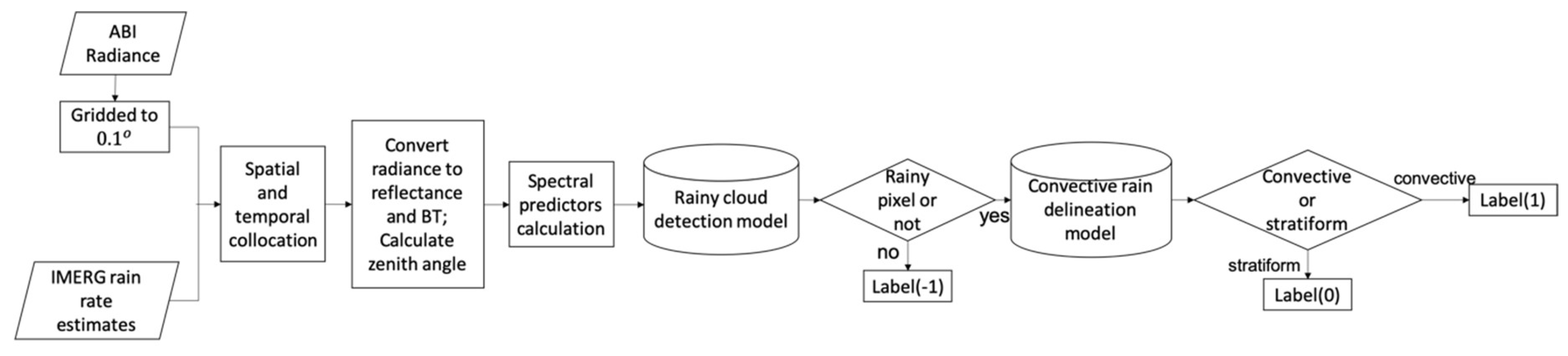
3.1. Data Processing

The goals of the automatic rainy cloud monitoring system are to detect rainy areas and delineate the convective areas. These two goals are achieved through the following steps:
  • Data preprocessing. First, the 16 bands of ABI radiance are gridded to the spatial resolution of 0.1°, the same as IMERG precipitation estimates. Second, six individual ABI data with scanning time ranges included in one IMERG time step are averaged to complete the spatial and temporal collocation between the two datasets. Third, Ref, BT, and sun zenith angle (z) are calculated, with reflectance being derived as follows (Equation (2)):
    Ref λ = L λ k ,
    where λ is the central wavelength of the channel, L λ is the radiance value, and κ is the reflectance conversion factor. The BT is derived from Equation (3) as follows:
    BT = [ fk 2 alog ( fk 1 L λ + 1 ) bc 1 ] / bc 2 ,
    where fk1, fk2, bc1, and bc2 are the Planck function constants. Sun zenith angle (z) is calculated through the variables in the ABI data file and pixel locations.
  • Spectral parameters are calculated and normalized.
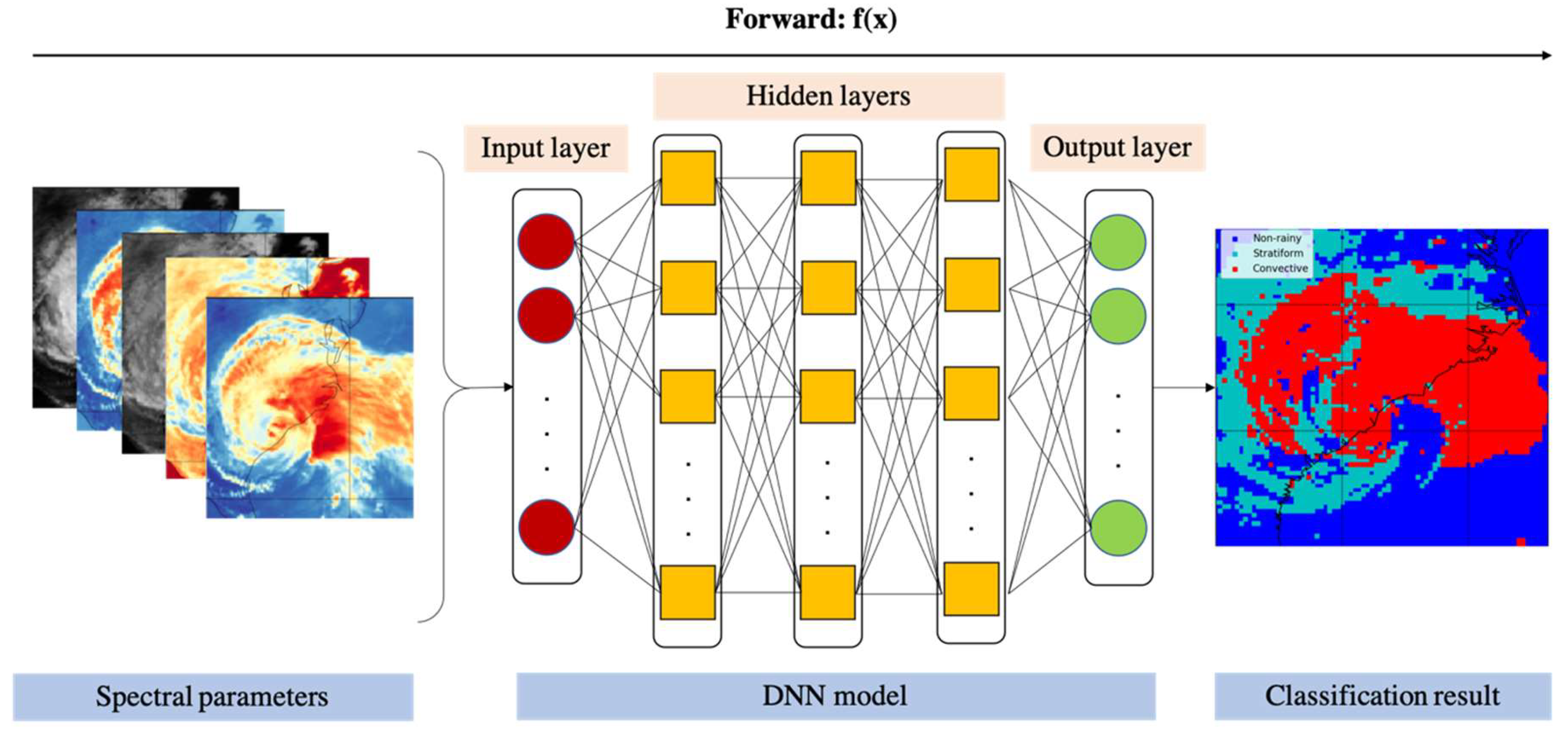
  • Each set of parameters is sorted into rainy and non-rainy clouds according to the associated IMERG rain rate (r). If r < 0.1 mm/hr, the sample is classified as non-rainy; otherwise, it is labeled as rainy. The rainy cloud detection models are built using DNN models, through which rainy samples are separated automatically from non-rainy ones.
    Sample {   R a i n y i f   r > = 0.1   m m / h r N o n r a i n y i f   r < 0.1   m m / h r
  • After rainy or non-rainy samples are distinguished, the convective and stratiform rain clouds are split based on their rain rates. The adopted threshold to discriminate convection or stratus cloud is calculated through the Z–r relation [49]:
    Z = 300 r 1.4 ,
    dBZ = 10 log 10 Z ,
    where Z ( m m 6   m 3 ) is the reflectivity factor of the radar, r (mm/hr) is the corresponding rain rate, and dBZ is the decibel relative to Z. Lazri [18] uses dBZ = 40 as the threshold of Z for convective precipitation. Then r is 12.24 mm/hr according to Equation (5). As precipitation rates measured by meteorological radar tend to be overestimated due to anomalous propagation of the radar beam [50], a lower threshold for r is more reasonable. This research uses r = 10 mm/hr as the final threshold because it is adopted frequently and has worked well in previous studies [20,51,52]:
    Sample {   C o n v e c t i v e i f   r > = 10   m m / h r S t r a t i f o r m i f   r < 10   m m / h r
  • Convective precipitation delineation models are built using training samples derived from step 4 with DNN models.
  • Accuracy is evaluated using validation data and case studies.
A flow chart of this procedure is illustrated in Figure 2.

3.2. Model Development

Following the data processing steps, the classification system contains two types of models: the rainy area detection and convective precipitation delineation models. This research adopts DNN methods to build both types of models and compares the performance with SVM and RF methods.
The DNN is a feed-forward artificial neural network with multiple hidden layers between the input and output [53]. The schematic workflow of the proposed DNN model (Figure 3) depicted in the input, hidden, and output layers forms a bipartite structure, with all these layers fully connected. The goal of this research is to detect the rainy cloud pixels and further classify them into two classes for each step. The DNN estimates the posteriors of each class given the input cloud features x, which refer to the spectral parameters. The activation functions used in each neuron of the hidden layers are rectified linear units (ReLUs) functions, which have the following advantages: (1) faster computation; and (2) more efficient gradient propagation [54]. The output is computed via the normalized exponential function to force the target label to have the maximum posterior estimation. The objective is to minimize the cross-entropy between predictions of DNN p = [p1, p2, … pJ]T and the target probabilities d = [d1, d2, ..., dJ ]T [55]. The loss function is defined in Equation (7):
L   =   j = 1 J d j log ( p j ) .
The back-propagation (BP) algorithm [56] is adopted to update the weights and bias of DNN based on the calculated loss.
The models achieve the optimal results when three hidden layers are embedded, and the numbers of neurons are 30, 20, and 20 for each hidden layer. For the rainy cloud detection models, “Yes” is returned when the pixel is identified as rainy and “No” for non-rainy. For the convective area delineation models, “Yes” is returned for convective pixels and “No” for stratiform. In applications, the non-rainy, stratiform, and convective pixels are labeled as −1, 0, and 1 in series.

4. Model Performance Evaluation

To include enough rainy and convective samples, training data were selected during rainy days from June to September of 2018, which contain at least one precipitation event for each day and have a large ensemble of different rain conditions. Eleven rainy days that do not overlap with training events were selected as testing samples (Table 3). Samples were randomly split into training (70%) and validation (30%) sets. The total number of pixels was 1,044,072.

4.1. Evaluation Metrics

This research uses the following statistical assessors to evaluate model accuracy, which are calculated in Equations (8)–(13):
  • The probability of detection (POD). The POD is the rate of testing samples correctly recognized as rainy/convective by the model:
    P O D   =   a a + c .
  • The probability of false detection (POFD). The POFD indicates the fraction of rainy/convective events incorrectly predicted by the model:
    P O F D   =   b b + d .
  • The false alarm ratio (FAR). The FAR is the ratio of the incorrect detection of rainy/convective pixels and the total pixels recognized as rainy/convective:
    F A R   =   b a + b .
  • The bias. Bias represents model over- or underestimates of reality:
    B i a s   =   a + b a + c .
  • The critical success index (CSI). The CSI is the fraction between the correct prediction of rainy/convective pixels by the model and the total number of pixels detected as rainy/convective by both IMERG and the model:
    C S I   =   a a + b + c .
  • The model accuracy (MA). The MA is the probability of a correct prediction of both rainy/convective and non-rainy/stratiform pixels by the model:
    M A   =   a + d a + b + c + d ,
    where the contingency parameters a, b, c, and d are summarized (Table 4).

4.2. Comparison of DNN, SVM, and RF Performance on Testing Data
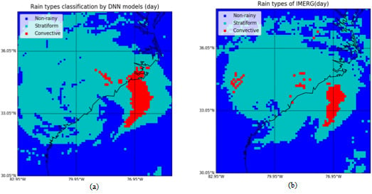
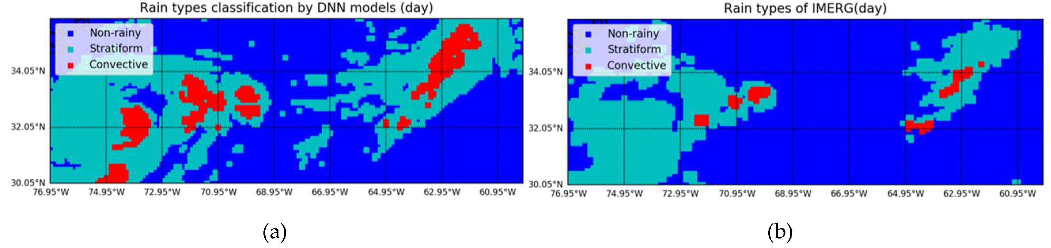
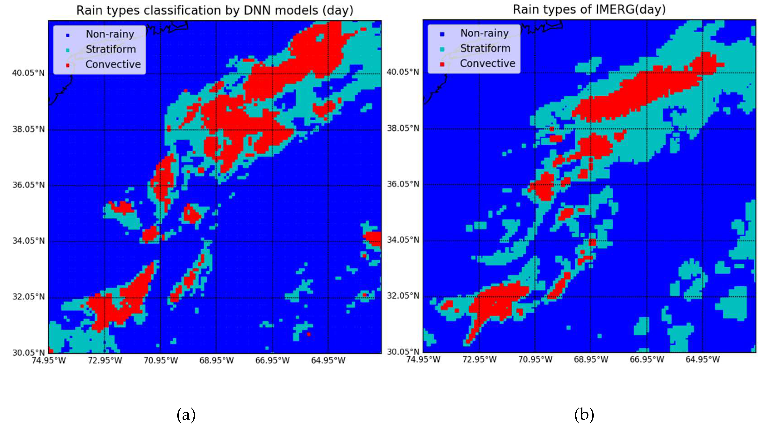
According to the assessors’ accuracies, the DNN system correctly detected most of the rainy areas (POD = 0.86 and CSI = 0.71) and convective areas (POD = 0.72 and CSI = 0.58), with relatively high overall accuracies (0.87 and 0.74, respectively). The research compared the performance of the DNN method with the other two machine learning methods, SVM and RF, and found that DNN performs better on the testing sets, especially in the delineation of convective precipitation.
For rainy area detection (Table 5), all three methods slightly overestimate the rainy pixels, while DNN achieved the highest accuracy in all the assessors. Overall, the performance of the three methods is similar, with no more than a 0.03 difference.
For convective precipitation delineation (Table 6), the advantage of DNN is even more evident, but all models overestimated the convective areas, except the DNN model. The DNN achieves the highest accuracy for almost all the assessors except POD (0.72 vs. 0.86 and 0.78). The DNN performed much better than RF and SVM, with a 0.20 lower FAR and 0.07–0.09 higher CSI. The SVM and RF significantly overestimated the convective pixels, with a FAR larger than 0.40.
The errors are mainly introduced by two sources. First, the acquisition time and frequency are different for ABI images and IMERG estimations. There are differences and gaps in scanning periods between ABI and the instruments used in IMERG data. Precipitation distribution and density may change and evolve in the periods. Second, since the ABI data have 0.5, 1, and 2 km spatial resolutions initially and are gridded to 0.1°, the spatial coverage is not the same for each set of spectral parameters and their associated rain rate. Errors also occur in the averaging process for spatial-temporal collocation.
Overall, the classification system efficiently detected the rainy area and extracted the convective areas from the testing dataset. In addition, most of the highest accuracies were observed in the proposed DNN models, being better performers than traditional machine learning when the data are complicated and sparsely distributed with a relatively large size [57]. The training and testing sample sizes were more than 500,000 and 50,000; on the other hand, there were 15 spectral parameters with different values for each pixel.

5. Case Study

Two case studies, a normal one and an extreme precipitation one (Hurricane Florence in 2018), were used to validate the performance of the classification system. Validation was carried out using only the DNN method due to its superior performance.

5.1. Normal Precipitation Events

Comparisons are shown between the predictions of the system and IMERG estimation of normal precipitation events for 9 July 2018 (Figure 4). The system accurately detected the rainy and convective area but slightly overestimated both. One possible reason is the temporal difference between the IMERG estimates and the ABI predicted results. The ABI data are temporally averaged from 13:30~14:00 UTC, whereas the IMERG data are retrieved at 14:00 UTC. Another reason is that the samples used in the training dataset were insufficient, which could be improved with the accumulation of the ABI data. Lastly, the thresholds that determine rain clouds are arbitrary, resulting in biases to their intercomparison result. Despite this shortcoming, the spatial distribution patterns of the predicted result and the IMERG data are congruent.
The results of a second case study of a normal precipitation event (9 September 2018) show that the system effectively identified the rainy areas and convective areas, with a minor underestimation of the rainy area and a minor overestimation of the convective areas (Figure 5).

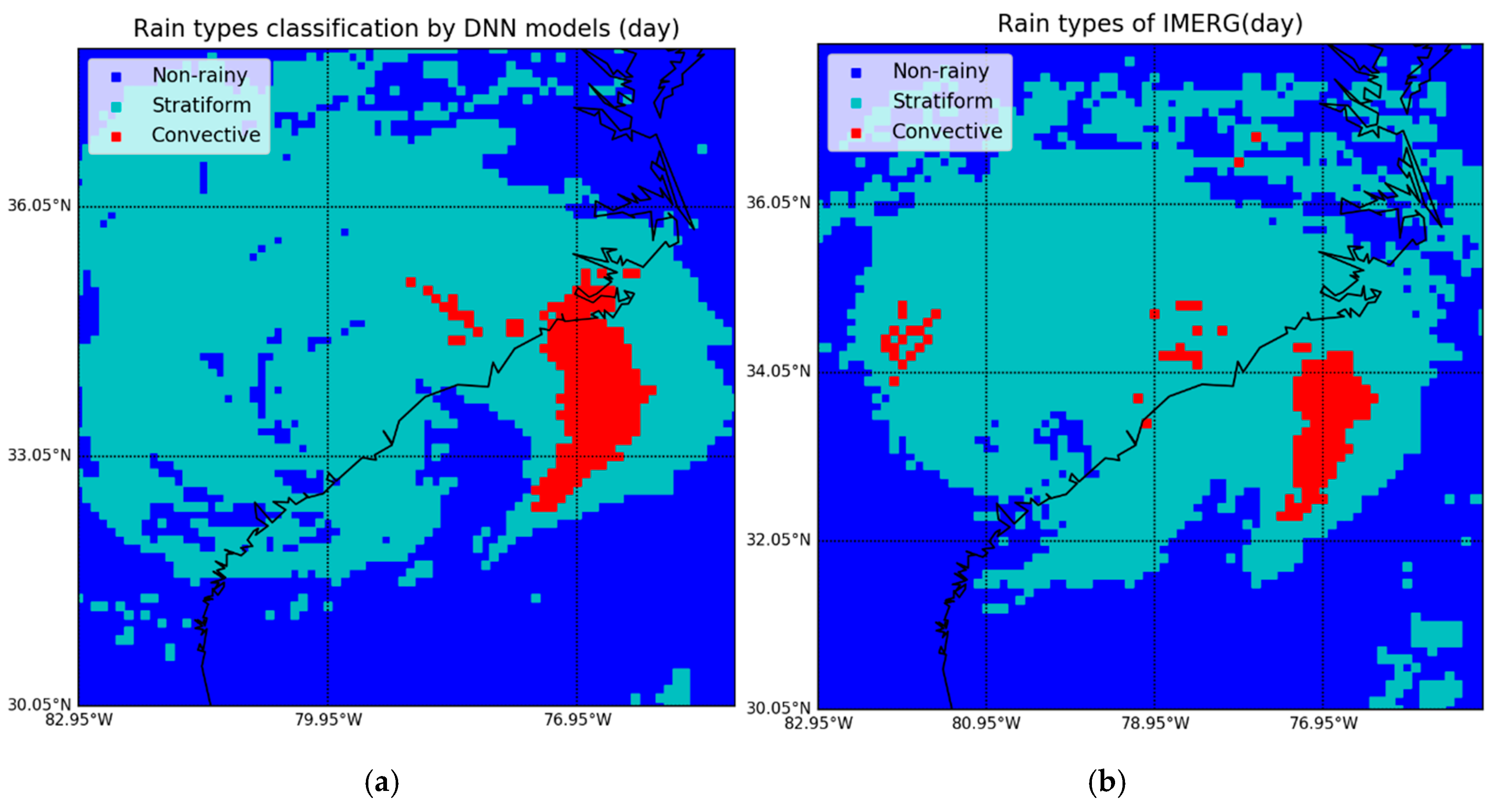
5.2. Hurricane Florence

The comparisons between the predictions of the system and IMERG estimations of Hurricane Florence demonstrate that the system detected most of the rainy areas, and the results clearly show the hurricane’s shape and area of influence (Figure 6). For the convective precipitation delineation, the models identify almost all of the convective areas. The system accurately detected the convective areas over the ocean, with a slight overestimation and some missed pixels over land. Overall, the system performed better over the ocean than land in the Hurricane Florence case study. Precipitation on land is influenced by more factors than over the ocean, including topography, land use, and vegetation [58]. The precipitation estimations of IMERG were calibrated by ground-based rain gauge data, and the measurements differ from those of the satellite-based system. In addition, different from normal precipitation events, hurricanes are extreme events where the clouds have more complicated air motion in both the horizontal and vertical dimensions. However, most samples used to train the models were normal precipitation, and Florence is the only hurricane event during the available period of ABI data in the study area. It is proposed that the models do not learn well about extreme events through the current data source.

6. Discussion

This research explores the performance of rainy cloud detection and convective precipitation delineation based on GOES-ABI data using the DNN method. The system detected rainy clouds with relatively high accuracy and is reliable for convective area extraction. However, overestimation is observed in the identification of convective precipitation, especially over land areas.
Due to the limitations of passive instrumentation, one of the recognized weaknesses in extracting cloud information from brightness temperature is that it only provides vertical column-integrated cloud information. Although the spectral parameters adopted in this research were effective in reflecting the information of LWP by using the differences in BTs, they do not measure raindrops in the cloud directly, as done by the PMW data. Therefore, the IR-BTD-based method does not perform well enough in deciding the rain rates. Overestimation of convective rain areas occurred in the validations and case studies.
However, the ABI data surpasses the PMW data in both spatial and temporal resolution and provides real-time monitoring and detection. The ABI’s temporal resolution is 5 minutes, and after the system is constructed, classification results are produced in the same interval. Conversely, the temporal resolution of IMERG is 30 minutes, six times less frequent than ABI. The system provides rainy cloud classification results at a spatial resolution of 2 km, five times greater than that of the IMERG data. It functions in the prediction of convective precipitation in both urgent precipitation hazards and routine weather forecasts and is an alternative when PMW data are unavailable.
Radar-based QPE offers a high-quality estimation of precipitation. However, ground-based radar is sparsely distributed and not available over the ocean, which has a high percentage of the heavy precipitation events (i.e., open ocean) and areas with the most significant economic impact (i.e., coasts). The GOES-ABI has full and continuous coverage of northern and southern America and large areas of the ocean. The system proposed herein complements the radar-based QPE over areas in which ground-based radar is unavailable.
To improve the performance of the proposed automatic detection system, several initiatives are envisioned. First, more spectral information is needed, especially those reflecting the features inside the clouds. This could be accomplished by adding an IR sounder, microwave images, and re-analysis of data like ECMWF (European Centre for Medium-Range Weather Forecasts) and MERRA2 (Modern-Era Retrospective Analysis for Research and Applications, Version 2). The second is better quality control in selecting rainy and convective pixels for training models. This may be addressed by adding more thresholds to the spectral parameters to further filter errors and bias. Thirdly, it is quite arbitrary to distinguish stratiform and convective precipitation solely using a fixed precipitation rate. This can be addressed by including more variables (e.g., pressure and temperature). The fourth is to extend the research to precipitation rate estimation and introduce AI methods, especially DL, to the transformation of statistical knowledge about meteorological phenomena into numerical models. This helps improve the accuracy of numerical weather predictions (NWPs). The fifth is that the precipitation product of Next Generation Weather Radar (NEXRAD) needs to be considered as validation data. The sixth focuses on the cloud types and precipitation conditions that differ under other climate regimes [59]. The models and system constructed in this research address only the daytime of the east coast of the U.S. Future investigations need to address separate classification systems for different areas of the U.S. and those happening during the nighttime.

7. Conclusions

This research proposes an automatic system of cloud classification based on the precipitation-producing capability to detect rainy clouds and delineate convective precipitation in real time, based on DNN technologies. The proposed DNN model returns better accuracies on the validation dataset, especially for convective precipitation delineation.
From the experiments and analysis, this research offers the following conclusions:
  • In the detection of rainy areas, the system provides reliable results of normal precipitation events and precipitation extremes such as hurricanes with a tendency toward overestimation;
  • The DNN achieves better performance than the two ML methods, with higher accuracies of the assessors on testing data;
  • The system performs better over the ocean versus land;
  • This study is offered as a contribution to combine the advantages of AI methodology with the modeling of atmospheric phenomena, a relatively innovative domain needing more exploration. More specifically, the system combines DNN-classifier and spectral features of rainy clouds to investigate precipitation properties. This research establishes an essential step with which to estimate precipitation rates further.

Author Contributions

Conceptualization, Q.L., Y.L., M.Y., L.S.C., X.H., C.Y. and D.Q.D.; writing—original draft preparation, Q.L., Y.L., M.Y. and L.S.C.; writing—review and editing C.Y., X.H. and D.Q.D.; funding acquisition, C.Y., L.S.C. and D.Q.D.

Funding

This research was funded by Ligado Networks (222992), NSF (1835507 and 1841520), and NASA (80NSSC19P2033).

Acknowledgments

NASA’s GODDARD Space Flight Center provided the IMERG data. The authors gratefully acknowledge Victoria Dombrowik from Yale University for reviewing the language of the paper, and the anonymous reviewers who have offered constructive feedback. A previous version of the paper was proofed by Professor George Taylor.

Conflicts of Interest

The authors declare no conflict of interest.

Abbreviations

ABIAdvanced Baseline Imager
AVHRRAdvanced Very High Resolution Radiometer
AVNNETAveraged neural networks
BPBack-propagation
CCDCold cloud duration
CCPDCold cloud phase duration
CMORPHClimate Prediction Center Morphing Technique
CONUSContiguous U.S.
CSICritical success index
CTTCloud-top temperature
dBZDecibel relative to reflectivity factor of the radar
DLDeep learning
DNNDeep neural network
FARFalse alarm ratio
GBRTGradient-boosted regression trees
IMERGIntegrated Multi-Satellite Retrievals for Global Precipitation Measurement
LWPLiquid water path
MAModel accuracy
MLMachine learning
MLPMultilayer perceptron network
NIRNear-infrared
NNETNeural networks
PMWPassive microwave
PODProbability of detection
POFDProbability of false detection
QPEQuantitative precipitation estimation
TRMMTropical Rainfall Measuring Mission

References

  1. Mason, D.; Speck, R.; Devereux, B.; Schumann, G.-P.; Neal, J.; Bates, P. Flood Detection in Urban Areas Using TerraSAR-X. IEEE Trans. Geosci. Remote. Sens. 2009, 48, 882–894. [Google Scholar] [CrossRef] [Green Version]
  2. Keefer, D.K.; Wilson, R.C.; Mark, R.K.; Brabb, E.E.; Brown, W.M.; Ellen, S.D.; Harp, E.L.; Wieczorek, G.F.; Alger, C.S.; Zatkin, R.S. Real-Time Landslide Warning During Heavy Rainfall. Science 1987, 238, 921–925. [Google Scholar] [CrossRef] [PubMed]
  3. Alfieri, L.; Thielen, J. A European precipitation index for extreme rain-storm and flash flood early warning. Meteorol. Appl. 2015, 22, 3–13. [Google Scholar] [CrossRef]
  4. Valipour, M. Optimization of neural networks for precipitation analysis in a humid region to detect drought and wet year alarms. Meteorol. Appl. 2016, 23, 1–100. [Google Scholar] [CrossRef]
  5. O’Gorman, P.A. Precipitation Extremes under Climate Change. Curr. Clim. Chang. Rep. 2015, 1, 49–59. [Google Scholar] [CrossRef] [PubMed]
  6. Wang, Z. The Impact of Extreme Precipitation on the Vulnerability of a Country. In IOP Conference Series: Earth and Environmental Science; IOP Publishing: Bristol, UK, 2018; Volume 170, p. 032089. [Google Scholar]
  7. Skofronick-Jackson, G.; Petersen, W.A.; Berg, W.; Kidd, C.; Stocker, E.F.; Kirschbaum, D.B.; Kakar, R.; Braun, S.A.; Huffman, G.J.; Iguchi, T.; et al. THE GLOBAL PRECIPITATION MEASUREMENT (GPM) MISSION FOR SCIENCE AND SOCIETY. Bull. Am. Meteorol. Soc. 2017, 98, 1679–1695. [Google Scholar] [CrossRef]
  8. Karbalaee, N.; Hsu, K.; Sorooshian, S.; Braithwaite, D. Bias adjustment of infrared-based rainfall estimation using Passive Microwave satellite rainfall data. J. Geophys. Res. Atmos. 2017, 122, 3859–3876. [Google Scholar] [CrossRef] [Green Version]
  9. Hong, Y.; Hsu, K.-L.; Sorooshian, S.; Gao, X. Precipitation Estimation from Remotely Sensed Imagery Using an Artificial Neural Network Cloud Classification System. J. Appl. Meteorol. 2004, 43, 1834–1853. [Google Scholar] [CrossRef] [Green Version]
  10. Thies, B.; Nauss, T.; Bendix, J. Discriminating raining from non-raining clouds at mid-latitudes using meteosat second generation daytime data. Atmos. Chem. Phys. Discuss. 2008, 8, 2341–2349. [Google Scholar] [CrossRef] [Green Version]
  11. Huffman, G.J.; Bolvin, D.T.; Nelkin, E.J.; Wolff, D.B.; Adler, R.F.; Gu, G.; Hong, Y.; Bowman, K.P.; Stocker, E.F. The TRMM Multisatellite Precipitation Analysis (TMPA): Quasi-Global, Multiyear, Combined-Sensor Precipitation Estimates at Fine Scales. J. Hydrometeorol. 2007, 8, 38–55. [Google Scholar] [CrossRef]
  12. Huffman, G.J.; Bolvin, D.T.; Nelkin, E.J. Integrated Multi-satellitE Retrievals for GPM (IMERG) technical documentation. NASA/GSFC Code 2015, 612, 47. [Google Scholar]
  13. Joyce, R.J.; Janowiak, J.E.; Arkin, P.A.; Xie, P. CMORPH: A Method that Produces Global Precipitation Estimates from Passive Microwave and Infrared Data at High Spatial and Temporal Resolution. J. Hydrometeorol. 2004, 5, 487–503. [Google Scholar] [CrossRef]
  14. Jensenius, J. Cloud Classification. 2017. Available online: https://www.weather.gov/lmk/cloud_classification (accessed on 17 April 2019).
  15. World Meteorological Orgnization. International Cloud Atlas. Available online: https://cloudatlas.wmo.int/clouds-supplementary-features-praecipitatio.html (accessed on 10 December 2019).
  16. Donald, D. What Type of Clouds Are Rain Clouds? 2018. Available online: https://sciencing.com/type-clouds-rain-clouds-8261472.html (accessed on 17 April 2019).
  17. Milford, J.; Dugdale, G. Estimation of Rainfall Using Geostationary Satellite Data. In Applications of Remote Sensing in Agriculture; Elsevier BV: Amsterdam, The Netherlands, 1990; pp. 97–110. [Google Scholar]
  18. Lazri, M.; Ameur, S.; Brucker, J.M.; Ouallouche, F. Convective rainfall estimation from MSG/SEVIRI data based on different development phase duration of convective systems (growth phase and decay phase). Atmospheric Res. 2014, 147, 38–50. [Google Scholar] [CrossRef]
  19. Arai, K. Thresholding Based Method for Rainy Cloud Detection with NOAA/AVHRR Data by Means of Jacobi Itteration Method. Int. J. Adv. Res. Artif. Intell. 2016, 5, 21–27. [Google Scholar] [CrossRef]
  20. Tebbi, M.A.; Haddad, B. Artificial intelligence systems for rainy areas detection and convective cells’ delineation for the south shore of Mediterranean Sea during day and nighttime using MSG satellite images. Atmospheric Res. 2016, 178, 380–392. [Google Scholar] [CrossRef]
  21. Mohia, Y.; Ameur, S.; Lazri, M.; Brucker, J.M. Combination of Spectral and Textural Features in the MSG Satellite Remote Sensing Images for Classifying Rainy Area into Different Classes. J. Indian Soc. Remote Sens. 2017, 45, 759–771. [Google Scholar] [CrossRef]
  22. Yang, C.; Yu, M.; Li, Y.; Hu, F.; Jiang, Y.; Liu, Q.; Sha, D.; Xu, M.; Gu, J. Big Earth data analytics: A survey. Big Earth Data 2019, 3, 83–107. [Google Scholar] [CrossRef]
  23. McGovern, A.; Elmore, K.L.; Gagne, D.J.; Haupt, S.E.; Karstens, C.D.; Lagerquist, R.; Smith, T.; Williams, J.K. Using Artificial Intelligence to Improve Real-Time Decision-Making for High-Impact Weather. Bull. Am. Meteorol. Soc. 2017, 98, 2073–2090. [Google Scholar] [CrossRef]
  24. Engström, A.; Bender, F.A.-M.; Charlson, R.J.; Wood, R. The nonlinear relationship between albedo and cloud fraction on near-global, monthly mean scale in observations and in the CMIP5 model ensemble. Geophys. Res. Lett. 2015, 42, 9571–9578. [Google Scholar] [CrossRef] [Green Version]
  25. Meyer, H.; Kühnlein, M.; Appelhans, T.; Nauss, T. Comparison of four machine learning algorithms for their applicability in satellite-based optical rainfall retrievals. Atmospheric Res. 2016, 169, 424–433. [Google Scholar] [CrossRef]
  26. LeCun, Y.; Bengio, Y.; Hinton, G. Deep learning. Nature 2015, 521, 436. [Google Scholar] [CrossRef] [PubMed]
  27. Liu, Q.; Chiu, L.S.; Hao, X.; Yang, C. Characteristic of TMPA Rainfall; American Association of Geographer Annual Meeting, Washington, DC, USA, 2019.
  28. Huffman, G.J.; Bolvin, D.T.; Braithwaite, D.; Hsu, K.; Joyce, R.; Xie, P.; Yoo, S.H. NASA Global Precipitation Measurement (GPM) Integrated Multi-satellitE Retrievals for GPM (IMERG). 2018. Available online: https://pmm.nasa.gov/sites/default/files/document_files/IMERG_ATBD_V5.2_0.pdf (accessed on 4 October 2019).
  29. Gaona, M.F.R.; Overeem, A.; Brasjen, A.M.; Meirink, J.F.; Leijnse, H.; Uijlenhoet, R.; Gaona, M.F.R. Evaluation of Rainfall Products Derived from Satellites and Microwave Links for The Netherlands. IEEE Trans. Geosci. Remote. Sens. 2017, 55, 6849–6859. [Google Scholar] [CrossRef]
  30. Wei, G.; Lü, H.; Crow, W.T.; Zhu, Y.; Wang, J.; Su, J. Comprehensive Evaluation of GPM-IMERG, CMORPH, and TMPA Precipitation Products with Gauged Rainfall over Mainland China. Adv. Meteorol. 2018, 2018, 1–18. [Google Scholar] [CrossRef] [Green Version]
  31. Benz, A.; Chapel, J.; Dimercurio, A., Jr.; Birckenstaedt, B.; Tillier, C.; Nilsson, W., III; Colon, J.; Dence, R.; Hansen, D., Jr.; Campbell, P. GOES-R SERIES DOCUMENTS. 2018. Available online: https://www.goes-r.gov/downloads/resources/documents/GOES-RSeriesDataBook.pdf (accessed on 3 August 2019).
  32. GOES-R Series Program Office. Goddard Space Flight Center. 2019. GOES-R Series Data Book. Available online: https://www.goes-r.gov/downloads/resources/documents/GOES-RSeriesDataBook.pdf (accessed on 10 December 2019).
  33. Cotton, W.; Bryan, G.; Heever, S.V.D. Storm and Cloud Dynamics; Academic press: Cambridge, MA, USA, 2010; Volume 99. [Google Scholar]
  34. Reid, J.S.; Hobbs, P.V.; Rangno, A.L.; Hegg, D.A. Relationships between cloud droplet effective radius, liquid water content, and droplet concentration for warm clouds in Brazil embedded in biomass smoke. J. Geophys. Res. Space Phys. 1999, 104, 6145–6153. [Google Scholar] [CrossRef]
  35. Chen, F.; Sheng, S.; Bao, Z.; Wen, H.; Hua, L.; Paul, N.J.; Fu, Y. Precipitation clouds delineation scheme in tropical cyclones and its validation using precipitation and cloud parameter datasets from TRMM. J. Appl. Meteorol. Clim. 2018, 57, 821–836. [Google Scholar] [CrossRef]
  36. Han, Q.; Rossow, W.B.; Lacis, A.A. Near-Global Survey of Effective Droplet Radii in Liquid Water Clouds Using ISCCP Data. J. Clim. 1994, 7, 465–497. [Google Scholar] [CrossRef] [Green Version]
  37. Nakajima, T.Y.; Nakajma, T. Wide-Area Determination of Cloud Microphysical Properties from NOAA AVHRR Measurements for FIRE and ASTEX Regions. J. Atmospheric Sci. 1995, 52, 4043–4059. [Google Scholar] [CrossRef] [Green Version]
  38. GOES-R ABI Fact Sheet Band 6 ("Cloud Particle Size" near-infrared). Available online: http://cimss.ssec.wisc.edu/goes/OCLOFactSheetPDFs/ABIQuickGuide_Band06.pdf (accessed on 4 October 2019).
  39. Vijaykumar, P.; Abhilash, S.; Santhosh, K.R.; Mapes, B.E.; Kumar, C.S.; Hu, I.K. Distribution of cloudiness and categorization of rainfall types based on INSAT IR brightness temperatures over Indian subcontinent and adjoiningoceanic region during south west monsoon season. J. Atmos. Solar Terr. Phys. 2017, 161, 76–82. [Google Scholar] [CrossRef]
  40. Scofield, R.A. The NESDIS Operational Convective Precipitation- Estimation Technique. Mon. Weather. Rev. 1987, 115, 1773–1793. [Google Scholar] [CrossRef]
  41. Giannakos, A.; Feidas, H. Classification of convective and stratiform rain based on the spectral and textural features of Meteosat Second Generation infrared data. In Theoretical and Applied Climatology; Springer: New York, NY, USA, 2013; Volume 113, pp. 495–510. [Google Scholar]
  42. Feidas, H.; Giannakos, A. Classifying convective and stratiform rain using multispectral infrared Meteosat Second Generation satellite data. In Theoretical and Applied Climatology; Springer: New York, NY, USA, 2012; Volume 108, pp. 613–630. [Google Scholar]
  43. Schmit, T.J.; Griffith, P.; Gunshor, M.M.; Daniels, J.M.; Goodman, S.J.; Lebair, W.J. A Closer Look at the ABI on the GOES-R Series. Bull. Am. Meteorol. Soc. 2017, 98, 681–698. [Google Scholar] [CrossRef]
  44. Thies, B.; Nauß, T.; Bendix, J.; Nauss, T. Precipitation process and rainfall intensity differentiation using Meteosat Second Generation Spinning Enhanced Visible and Infrared Imager data. J. Geophys. Res. Space Phys. 2008, 113. [Google Scholar] [CrossRef]
  45. Baum, B.A.; Soulen, P.F.; Strabala, K.I.; Ackerman, S.A.; Menzel, W.P.; King, M.D.; Yang, P. Remote sensing of cloud properties using MODIS airborne simulator imagery during SUCCESS: 2. Cloud thermodynamic phase. J. Geophys. Res. Space Phys. 2000, 105, 11781–11792. [Google Scholar] [CrossRef]
  46. Baum, B.A.; Platnick, S. Introduction to MODIS cloud products. In Earth Science Satellite Remote Sensing: Science and Instruments; Qu, J.J., Gao, W., Kafatos, M., Murphy, R.E., Salomonson, V.V., Eds.; Springer: New York, NY, USA, 2006. [Google Scholar]
  47. Kuligowski Robert, J. GOES-R Advanced Baseline Imager (ABI) Algorithm Theoretical Basis Document for Rainfall Rate (QPE). 2010. Available online: https://www.star.nesdis.noaa.gov/goesr/documents/ATBDs/Baseline/ATBD_GOES-R_Rainrate_v2.6_Oct2013.pdf (accessed on 4 October 2019).
  48. Hartmann, D.L. Global Physical Climatology, 2nd ed.; Academic Press: Cambridge, MA, USA, 1994. [Google Scholar]
  49. Hunter, S.M. WSR-88D radar rainfall estimation: Capabilities, limitations and potential improvements. Natl. Wea. Dig. 1996, 20, 26–38. [Google Scholar]
  50. Islam, T.; Rico-Ramirez, M.A.; Han, D.; Srivastava, P.K. Artificial intelligence techniques for clutter identification with polarimetric radar signatures. Atmospheric Res. 2012, 109, 95–113. [Google Scholar] [CrossRef]
  51. Baquero, M.; Cruz-Pol, S.; Bringi, V.; Chandrasekar, V. Rain-rate estimate algorithm evaluation and rainfall characterization in tropical environments using 2DVD, rain gauges and TRMM data. In Proceedings of the 25th Anniversary IGARSS 2005 IEEE International Geoscience and Remote Sensing Symposium, Seoul, Korea, 29–29 July 2005; Volume 2, pp. 1146–1149. [Google Scholar]
  52. Maeso, J.; Bringi, V.; Cruz-Pol, S.; Chandrasekar, V. DSD characterization and computations of expected reflectivity using data from a two-dimensional video disdrometer deployed in a tropical environment. In Proceedings of the 25th Anniversary IGARSS 2005 IEEE International Geoscience and Remote Sensing Symposium, Seoul, Korea, 29–29 July 2005; pp. 5073–5076. [Google Scholar]
  53. Qian, Y.; Fan, Y.; Hu, W.; Soong, F.K. On the training aspects of deep neural network (DNN) for parametric TTS synthesis. In Proceedings of the 2014 IEEE International Conference on Acoustics, Speech and Signal Processing (ICASSP), Florence, Italy, 4–9 May 2014; pp. 3829–3833. [Google Scholar]
  54. Dahl, G.E.; Sainath, T.N.; Hinton, G.E. Improving deep neural networks for LVCSR using rectified linear units and dropout. In Proceedings of the 2013 IEEE International Conference on Acoustics, Speech and Signal Processing, Vancouver, BC, Canada, 26–31 May 2013; pp. 8609–8613. [Google Scholar]
  55. Xu, Y.; Huang, Q.; Wang, W.; Plumbley, M.D. Hierarchical learning for DNN-based acoustic scene classification. arXiv 2016, arXiv:1607.03682. [Google Scholar]
  56. Hinton, G.; Deng, L.; Yu, D.; Dahl, G.; Mohamed, A.R.; Jaitly, N.; Senior, A.; Vanhoucke, V.; Nguyen, P.; Kingsbury, B.; et al. Deep neural networks for acoustic modeling in speech recognition. IEEE Signal Process. Mag. 2012, 29, 82–97. [Google Scholar] [CrossRef]
  57. Caruana, R.; Niculescu-Mizil, A. An empirical comparison of supervised learning algorithms. In Proceedings of the 23rd International Conference on Machine Learning, Pittsburgh, PA, USA, 25–29 June 2006; pp. 161–168. [Google Scholar]
  58. Rodgers, E.; Siddalingaiah, H.; Chang, A.T.C.; Wilheit, T. A Statistical Technique for Determining Rainfall over Land Employing Nimbus 6 ESMR Measurements. J. Appl. Meteorol. 1979, 18, 978–991. [Google Scholar] [CrossRef] [Green Version]
  59. Berg, W.; Kummerow, C.; Morales, C.A. Differences between East and West Pacific Rainfall Systems. J. Clim. 2002, 15, 3659–3672. [Google Scholar] [CrossRef] [Green Version]
Figure 1. Geographic coverage of study area.
Remotesensing 11 02555 g001
Figure 2. Workflow of the automatic rainy cloud classification system. IMERG is Integrated Multi-Satellite Retrievals for Global Precipitation Measurement; BT is Brightness Temperature.
Remotesensing 11 02555 g002
Figure 3. Flowchart of the deep neural network (DNN) model for cloud classification and delineation.
Remotesensing 11 02555 g003
Figure 4. Cloud classification results and IMERG estimations on normal precipitation: (a) ABI prediction; and (b) IMERG estimation on 9 July 2018, at 13:30–14:00 UTC.
Remotesensing 11 02555 g004
Figure 5. Cloud classification results and IMERG estimations of normal precipitation: (a) ABI prediction; and (b) IMERG estimation on 19 September 2018, at 18:00–18:30 UTC.
Remotesensing 11 02555 g005
Figure 6. Cloud classification results and IMERG estimations of Hurricane Florence: (a) ABI; and (b) IMERG estimation on 15 September 2018, at 18:00–18:30 UTC.
Remotesensing 11 02555 g006
Table 1. Advanced Baseline Imager (ABI) band characteristics.
Band NumberCentral Wavelength (μm)Spatial Resolution at Nadir (km)κ-Factor
(W −1 * m * μm)
Used in StudyPrimary Application
10.471.01.5177−3 Aerosols
20.640.51.8767−3Clouds
30.8651.03.1988−3Vegetation
41.3782.08.4828−3 Cirrus
51.611.01.26225−2 Snow/ice discrimination, cloud phase
62.242.03.98109−2Cloud particle size, snow cloud phase
73.92.0- Fog, stratus, fire, volcanism
86.192.0-Various atmospheric features
96.952.0- Middle-level water vapor features
107.342.0-Lower-level water vapor features
118.52.0-Cloud-top phase
129.612.0-Total column of ozone
1310.352.0-Clouds
1411.22.0-Clouds
1512.32.0-Clouds
1613.32.0-Air temperature, clouds
Table 2. Spectral parameters used in the models, with the subscript number being the central wavelength (μm).
Spectral ParametersCloud Features Reflected by the Parameter
Ref0.64Cloud brightness
Ref0.865Cloud brightness
Ref2.24Cloud particle size
BT10.35Cloud particle size, cloud-top temperature
ΔBT6.19−10.35Cloud-top temperature, convective level
ΔBT7.34−12.3Cloud-top temperature, convective level
ΔBT6.19−7.34Cloud height and thickness
ΔBT13.3−10.35Cloud-top height
ΔBT9.61−13.3Cloud-top height
ΔBT8.5−10.35Cloud phase (positive for thick ice clouds, negative for thin low-level water clouds)
ΔBT8.5−12.3Optical thickness (negative values for thin optical thickness)
BT6.19Upper-level tropospheric water vapor
ΔBT7.34−8.5Cloud optical thickness
ΔBT7.34−11.2Cloud-top temperature and height
ΔBT11.2−12.3Cloud thickness, particle size
Table 3. Dates of precipitation events in training and testing data.
Training and Validation SamplesTesting Samples
3–5, 17, 22 June; 1, 10, 24 June;
4, 7, 30, 31 July; 11, 26 July;
2–4, 8–12, 18–20, 22 August; 5–7 August;
7–8, 14, 17, 25 September4–6 September
Table 4. Contingency parameters of the statistical assessors.
By IMERG
Yes (Rainy/Convective)No (Non-Rainy/Stratiform)
By modelsYes (Rainy/Convective)ab
No (Non-rainy/Stratiform)cd
Table 5. Validation of rainy cloud detection model on testing data. The best result for each assessor is shown in bold. POD is the Probability of Detection; POFD is the Probability of False Detection; FAR is False Alarm Ratio; CSI is the Critical Success Index; MA is the Model Accuracy; DNN is Deep Neural Network; SVM is Support Vector Machine; RF is Random Forest.
ModelPOD
(Ideal 1)
POFD
(Ideal 0)
FAR
(Ideal 0)
Bias
(Ideal 1)
CSI
(Ideal 1)
MA
(Ideal 1)
DNN0.860.130.201.070.710.87
SVM0.850.130.211.070.690.86
RF0.850.140.211.090.700.86
Table 6. Validation of convective precipitation delineation model on testing data. The best result for each assessor is shown in bold.
ModelPOD
(Ideal 1)
POFD
(Ideal 0)
FAR
(Ideal 0)
Bias
(Ideal 1)
CSI
(Ideal 1)
MA
(Ideal 1)
DNN0.720.230.240.940.580.74
SVM0.860.400.441.550.510.69
RF0.780.350.431.370.490.70

