waveformlidar: An R Package for Waveform LiDAR Processing and Analysis

Abstract

A wealth of Full Waveform (FW) LiDAR (Light Detection and Ranging) data are available to the public from different sources, which is poised to boost extensive applications of FW LiDAR data. However, we lack a handy and open source tool that can be used by potential users for processing and analyzing FW LiDAR data. To this end, we introduce waveformlidar, an R package dedicated to FW LiDAR processing, analysis and visualization as a solution to the constraint. Specifically, this package provides several commonly used waveform processing methods such as Gaussian, Adaptive Gaussian and Weibull decompositions and deconvolution approaches (Gold and Richard-Lucy (RL)) with users’ customized settings. In addition, we also developed functions to derive commonly used waveform metrics for characterizing vegetation structure. Moreover, a new way to directly visualize FW LiDAR data is developed by converting waveforms into points to form the Hyper Point Cloud (HPC), which can be easily adopted and subsequently analyzed with existing discrete-return LiDAR processing tools such as LAStools and FUSION. Basic explorations of the HPC such as 3D voxelization of the HPC and conversion from original waveforms to composite waveforms are also available in this package. All of these functions are developed based on small-footprint FW LiDAR data but they can be easily transplanted to the large footprint FW LiDAR data such as Geoscience Laser Altimeter System (GLAS) and Global Ecosystem Dynamics Investigation (GEDI) data analysis. It is anticipated that these functions will facilitate the widespread use of FW LiDAR and be beneficial for better estimating biomass and characterizing vegetation structure at various scales.

1. Introduction

The advent of Full Waveform (FW) LiDAR (Light Detection and Ranging) data including airborne and spaceborne have enabled new opportunities for vegetation structure characterization at a range of scales [1,2,3,4,5]. Unlike Discrete-return (DR) LiDAR data which only store the crest of analog signal representing discrete echo, FW LiDAR data can store the entire echo scattered from illuminated objects with different temporal resolutions [1,6]. This advantage provides more information about the objects that the pulse interacts with and gives users more flexibility to interpret information inherent in waveforms [7].

Multiple approaches such as the Gaussian decomposition and deconvolution have been developed to interpret information from waveforms [6,8,9]. However, complicated processing steps and algorithms hinder the widespread use of Full Waveform (FW) LiDAR data. To tackle these challenges, our package waveformlidar proposed several commonly used approaches and functions to conduct waveform processing and analysis such as Gaussian decomposition and deconvolution. These approaches have been successfully applied to extract physical attributes of vegetation such as canopy height, stem volume, aboveground biomass and tree species from LiDAR waveforms [2,3,10]. With the aid of the package, these approaches can be easily implemented in the R platform and further relieve users’ concerns on complicated FW processing steps.

Additionally, currently available tools are mainly oriented for processing DR LiDAR data. There is a lack of handy tools that dedicated to FW LiDAR data, which precludes users to explore the new or potential practices of FW LiDAR data. Therefore, we developed functions to derive commonly used waveform metrics such as front slope and waveform distance. These waveform metrics are different from the metrics derived from waveform decomposition in terms of the information they contained. Thus, they can be complementary to metrics obtained from decomposition, which enable users to make the most use of the waveform information contained [11].

Lastly, the package also proposed a new method to convert waveforms into point clouds with hyper point density (Hyper Point Cloud, HPC) and composite waveforms after implementing waveform voxelization steps. The HPC is an alternative product of FW LiDAR data, which not only can preserve information embedded in original waveforms, also offer users a convenient way to visualize and decode information with existing LiDAR processing tools such as LAStools [12] and FUSION [13]. However, not every waveform signal is useful for real-world applications. To explore the HPC’s potential usefulness, this package also provides functions to explore the HPC in 2D and 3D spatial dimensions. Additionally, we also explore the methods to convert original waveforms with waveform intensities distributing at an off-nadir angle into composite waveforms with intensities distributing at the vertical direction. Furthermore, we conducted a comparison between original waveforms and composite waveforms on the tree species identification and detailed information can be found in Zhou et al. [11]. Notably, the storage and computation cost using the composite waveforms is more expensive than original waveforms, which requires users to conduct an assessment of the marginal benefits obtained from composite waveforms.

Overall, the purpose of this article is to provide an overview of the waveformlidar package and to ensure the free availability and usability of methodologies including code or algorithms from our previous scholarly publications. We first introduce an example of FW LiDAR data and corresponding ancillary data such as outgoing pulse and system impulse data. Next, we begin to briefly explain the main algorithms’ technical principles and the logic behind them. We end by discussing the main functions such as decomposition, deconvolution and the HPC in the practical use in the R platform. Full tutorials and reports to reproduce the results from these examples are available in the supporting information from our website (https://github.com/tankwin08/waveformlidar/vignettes).

2. Example Datasets

FW LiDAR data are available on the market with various formats. However, they are primarily composed of two parts—a geolocation part that keeps geo-reference locations derived from range measurement between the laser sensor and the reference location and a wave part which stores digitized return energy starting from the reference location till the end of digitized samples [4]. To mitigate the effect of format on the FW LiDAR data processing, we converted these files into CSV format and then conducted the subsequent analysis. The waveform LiDAR datasets were downloaded from National Ecological Observatory Network (NEON) data center (http://www.neonscience.org/content/airborne-data). The example dataset used here is a subset (500 waveforms) from the Harvard Forest, Massachusetts, USA. Each row represents one waveform and each column represents a time bin. The temporal resolution of the time bin can be 1/2/4 nanosecond (ns), which is up to the data collecting system. In this case, the temporal resolution is 1 ns with the vertical distance approximately 0.15 m.

Overall, there are two major methods for waveform processing in this package. The first method was direct decomposition (I), which only applied the Gaussian, Adaptative Gaussian and Weibull models to decompose waveform data. The second method was the deconvolution and then decomposition (II) method. More details of these two methods can be found in Zhou et al. (6). Brief introduction of these two methods are elaborated in the Methods section. Most of the functions in the waveformlidar package require waveform LiDAR data as the input for obtaining useful information. However, the method II requires additional input data such as corresponding outgoing pulse data, system response impulse and its corresponding outgoing pulse to interpret information inherent in waveforms. Ideally, the system response pulse would be measured in the lab using a hard target. Here, a provisional system response impulse was provided. It was a return pulse of a single laser shot from a hard ground target with a mirror angle close to nadir [6]. Through deconvolving the outgoing pulse corresponding to this provisional system response pulse, we can obtain an estimated system response pulse closer to the “true” system response pulse. With the aid of the estimated system response impulse, the system response effect can be removed with the deconvolution method. Alternatively, the provisional system response pulse can be used as “true” system response pulse when no corresponding outgoing pulse was provided. In the Deconvolution section, we provided an example to show the detailed deconvolution process. In addition, we also provided two example results with the two different methods. In summary, we provided 8 datasets in this package and their corresponding brief introduction as shown in

Table 1. A summary of example data sets for waveformlidar package.

Dataset Names	Physical Meaning	Size (Row*Column)	Data Type
return	FW lidar data	500*208	Data frame
outg	Outgoing pulse corresponding to return	500*100	Data frame
imp	Return impulse response	100	Numeric vector
imp_out	Outgoing pulse corresponding to imp	100	Numeric vector
geo	Geo-reference data corresponding to return	500*16	Data frame
decom_result	Sample results after direct decomposition method	1000*7	Data frame
decon_result	Sample results after decomposition and deconvolution method	1000*7	Data frame
shp_hf	An polygon of small boundary in Harvard Forest, Massachusetts, USA	Vector	Vector or shapefile

.

3. Methods and Functions

3.1. Methods

3.1.1. Decomposition and Deconvolution

The waveformlidar package provides two broad sets of methods including the deconvolution and decomposition to interpret useful information from waveform LiDAR data. These two methods are built on different assumptions. For the deconvolution (Equation (1)), we assumed that the returning pulses of the waveform were the product of interaction among outgoing pulses, atmospheric scattering, system noise and reflecting surfaces. In other words, the return waveform can be expressed as the convolution of the outgoing pulse, impulse response (atmospheric scattering, system noise, etc.) and effective target cross section [6,7] (Equation (1)).

$$P_r\left(t\right)={\displaystyle \sum }_{i=1}^n\frac{D^2}{4\pi {\gamma }^2{R}_i{}^4}{P}_t\left(t\right)\ast \tau \left(t\right)\ast {\delta }_i\left(t\right)$$

(1)

where $P_r^t\left(t\right)$ is the received laser power, $P_t\left(t\right)$ is the emitted laser power,$\mathsf{\tau }\left(\mathrm{t}\right)$ is the receiver impulse function, D is the aperture diameter of the receiver optics, λ is the wavelength, R is the range from the LiDAR system to the target, n is the number of the effective target cross sections and ${\delta }_i\left(t\right)$ is the ith effective target cross section.

Thus, the deconvolution is an algorithm-based process that is to reverse the effect of convolution on the recorded signals and the decomposition is a process which can provide estimates of the location and properties of objects along the pulse [7]. In this package, two deconvolution methods including the Gold and Richardson-Lucy (RL) are available for conducting the deconvolution. The detailed description of these algorithms can be found in Reference [6].

For the decomposition (Equations (2)–(4)), both the outgoing pulse and the return pulse are nearly following some probability distribution such as Gaussian distribution in terms of shape. Thus, the information inherent in waveform can be extracted through fitting waveforms with a mixture of models with the specific distribution or waveform components. By interpreting these models’ parameters or waveform components, the targets such as vegetation and ground interacting with outgoing pulse along the path can be characterized.

In this package, three representative models such as the Gaussian (Equation (2)), Adaptative Gaussian (Equation (3)) and Weibull (Equation (4)) models [4,9] were available to interpret information from waveforms. The Gaussian model is the most frequently used model for waveform decomposition. In general, the outgoing pulse is assumed to be Gaussian shape, as well as the effective target cross-section [7]. The return waveform is obtained through the convolution of these two, which result in the return waveform also follows the Gaussian distribution in the ideal condition. Therefore, the return waveform can be fitted with a mixture of Gaussian models. $\theta$ are parameters for each model.

$$f\left(x,\theta \right)={\displaystyle \sum }_{i=1}^n{A}_i\exp \left(-\frac{{\left(x-{\mu }_i\right)}^2}{2{\sigma }_i{}^2}\right)$$

(2)

where n is the number of Gaussian components, $A_i$ is the amplitude of ith waveform component, ${\delta }_i$ is the standard deviation of ith waveform component and ${\mu }_i$ is the time location of ith waveform component.

The Adaptive Gaussian model has the form of Equation (3) which can minimize the residual of the model by introducing another variable which is also known as rate parameter (λ).

$$f\left(x,\theta \right)={\displaystyle \sum }_{i=1}^n{A}_i\exp \left(-\frac{{\left(x-{\mu }_i\right)}^{\lambda }}{2{\sigma }_i{}^2}\right)$$

(3)

The Weibull model (Equation (4)) was introduced since it enables us to simulate either symmetric or asymmetric peaks with four unknown parameters [4].

$$f\left(x,\theta \right)={\displaystyle \sum }_{i=1}^n{A}_i\frac{\mathrm{k}}{{\delta }_i}{\left(\frac{x-{\mu }_i}{{\sigma }_i}\right)}^{k-1}\exp \left(-{\left(\frac{x-{\mu }_i}{{\sigma }_i}\right)}^k\right)$$

(4)

where A_i is the amplitude, k (> 0) is the shape parameter that controls the behavior or the shape of the distribution and σ_i (> 0) is the scale parameter that controls the spread of the distribution. The shape parameter can capture the asymmetry or skewness of the waveforms that overcomes the disadvantage of the Gaussian function, which is only suitable for symmetric distributions. ${\mu }_i$ is a location parameter in the Weibull model.

3.1.2. Hyper Point Cloud

The methods mentioned in Section 3.1.1 are mainly intended to convert part of waveform signals into points to form DR-like point clouds with additional information such as amplitude (A) and echo width ($\delta$). However, intensity information embedded in waveforms, which is the most conspicuous advantage of FW LiDAR data, is still insufficiently studied. Moreover, the decomposition or deconvolution method requires users to have a deep understanding of complicated waveform processing methods and precludes practitioners’ willingness to explore FW LiDAR data’s potential. To overcome these technical barriers and make the most use of waveform information, we proposed a new concept named Hyper Point Cloud (HPC) to directly convert all waveform information into points with the aid of the geo-reference data [14]. In addition, this product also renders us a direct way to visualize the FW LiDAR data with existing tools or software mainly oriented toward DR LiDAR data processing.

Beyond the concept of the HPC, we also developed some algorithms to explore potential applications of the HPC. For example, the waveformgrid and waveformvoxel are primarily meant to generalize information at the 2D and 3D spatial scale from the HPC. The logic of these two is to project waveform information into 2D grid cells or voxels to obtain high-level information of objects according to the user defined resolution. Furthermore, we also developed an algorithm (rawtocomposite) to generate composite waveforms with waveform signals that are vertically distributed. It is anticipated that this product can reduce the impact of tilt angle on the vegetation characterization in the vertical direction.

To get a better overview of our package, we summarized the major functions in

Table 2. Summary of major functions of waveformlidar package.

Package	Categories	Functions
	Waveform processing	decom
		decom.adaptive
		decom.weibull
		deconvolution …
waveformlidar	Waveform variables extraction	fslope
		percentile.location
		ground.location
		integral
		waveformclip …
	Hyper point cloud	hyperpointcloud
		waveformgrid
		waveformvoxel
		rawtocomposite …

.

3.2. Functions with Examples

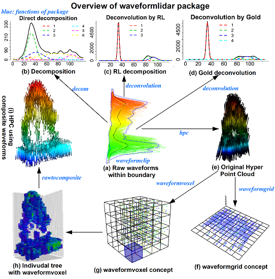
As shown in Table 2, the waveformlidar package consists of three major components—waveform processing, waveform variable extraction and HPC generation and its potential applications. More specifically, we summarized core functions of the package in Figure 1. For example, the decom is used for decomposition, the deconvolution is used for Gold and RL deconvolution, hpc is used for generating the HPC, waveformgrid and waveformvoxel is used for projecting the HPC into 2D and 3D dimensions and rawcomposite is used for generating composite waveforms from the HPC. The core these functions of the package and how to use them are elaborated in the following sections.

3.2.1. Installation

To install the latest release version from CRAN, type install.packages(“waveformlidar”) within R. The current developmental version can be downloaded from GitHub via:

if (!require(“devtools”)) {

  install.packages(“devtools”)

}

devtools::install_github(“tankwin08/waveformlidar”, dependencies = TRUE)

3.2.2. Preprocessing

The waveform processing involves a series of preprocessing steps such as noise detection, smoothing and radiometric calibration. In this package, we provide some options in several functions to conduct the preprocessing steps.

Different data sources may store data in different radiometric resolution or start at different baseline values. For instance, the NEON FW LiDAR data are 16 bits and the baseline value of the waveform is about 200. To optimize subsequent analysis, we applied the minimum subtraction for each waveform to ensure that the signal intensity starts at 1.

Before conducting waveform processing with the decomposition or deconvolution methods, several functions are also available to obtain general information about the waveform echoes. For example, the lpeak function can be used to identify the peak location in each waveform with TRUE and FALSE; the npeaks function is to identify the number of waveform components (n) of models being used. Another important function is the gennls, which is used to generate the non-linear Gaussian model formula for each waveform based on the number of waveform components and the probability distribution model the users chose. Moreover, this function also gives the model appropriate initiated estimates for parameters such as $A_i$, ${\mu }_i$ and ${\sigma }_i$ to ensure the successful solutions of waveform fitting. For example, if one waveform was identified with the three waveform components and the corresponding initialized parameters are given as follows:

library(waveformlidar)

A<-c(76,56,80); mu<-c(29,40,67); sig<-c(4,3,2.5)

The Gaussian model can be generated automatically with these known parameters.

fg<-gennls(A,mu,sig)

fg returns two parts—fg$formula gives the formula of the Gaussian model and fg$start provides the initiated values for each parameter based on known values.

The models suitable for the waveform fitting are the non-linear models that generally suffer from the problem of non-uniqueness, which indicates that there are several possible models could be used for fitting one waveform. Thus, this package also provides another two representative models such as the Adaptative Gaussian (agennls) and Weibull functions (wgennls) to generate formulas and initiate parameters for the model fitting. These two functions both have four parameters which require us to give four vectors to initiate parameter estimates. The only difference between the Gaussian function and Adaptive Gaussian function is the rate parameter r. When r = 2, the adaptive Gaussian function becomes the Gaussian function. For example, the Adaptive Gaussian model given the three waveform components can be generated as follows:

A<-c(76,56,80); mu<-c(29,40,67); sig<-c(4,3,2.5);  r<-c(2,2,2)

afg<- agennls(A,mu,sig,r)

afg$formula

The Weibull function also has four parameters but their physical meanings are different from the Gaussian and adaptive Gaussian functions. The detailed description of these parameters can be found in the study of Zhou and Popescu [4].

In addition to using models to decompose waveforms, a function named peakfind is also available to roughly estimate the parameters based on waveform shapes.

rough_estimates<- peakfind(wf[182,])

In the matrix of rough_estimates, the number of rows represents the number of waveform components and the columns corresponds to the index number of the waveform, the estimated amplitude, time location(s) and echo width(s) of the corresponding waveform component(s). As shown in Figure 2a, the green circles (I) represent the estimated amplitude, the vertical blue dash lines (m) represent the corresponding time locations and the horizontal dash lines (s) represent the roughly estimated echo widths (not real echo width). With the default, we can obtain four sets of parameters for four waveform components (peaks). In fact, the first peak parameters may be caused by noise.

Actually, most of the waveforms are mixed with noise as we have shown in Figure 2b. There is a difference between the ideal Gaussian waveform (IGW, black dash line, generated from a mixture of Gaussian functions) and the raw waveform (RW, red). Consequently, some unreasonable peaks maybe detected when the RWs mixed with a high level of noise. To obtain more reasonable results, we need to conduct some preprocessing steps such as smoothing and threshold filtering. For example, we increased the threshold to 0.3 to achieve a more reasonable rough estimate (rough_estimates1).

rough_estimates1<- peakfind (wf[182, ],  thres = 0.3)

3.2.3. Decomposition

Similar to the peakfind function, our core function decom also had an option named thres to enable users to specify the threshold (thres*maximum intensity of the given waveform) for selecting peaks and determine the number of waveform components. Another two important arguments are smooth and width which are used to determine if we applied mean filter and the width of mean filter to reduce the negative effect of noise on the waveform decomposition. The default is to use the smooth function with the width = 3. The width argument is valid only when the smooth = TRUE.

For an individual waveform, we can implement the following codes to obtain the decomposition result using the smoothed waveform (r1) and the raw waveform (r2).

r1<- decom(wf[1,])

r2<- decom(wf[1,], smooth = FALSE)

Results of decomposition are stored in a list, which consists of three components—the first is the index of waveform for tracking the results from each waveform; the second is the raw results with all estimated parameters; the third one is to extract parameters from the second result such as estimates and standard error of the estimates, which is mainly to prepare for calculating the point cloud from the decomposition results.

Results of r1 and r2 showed almost the same parameter estimates using smoothed and raw waveforms. However, the decomposition results using the raw waveform may not give you a solution to the “complex” waveform data fitting with an amount of noise. Generally, it was expected that 1–2% of waveform data were in this kind of conditions based on past experience. The following example showed one waveform with an amount of noise. The decomposition of r3 just returns NULL due to the waveform being extremely irregular or to the user rendering inappropriate initiating parameters. However, the decomposition results can be achieved through adjusting the thres option such as smooth options (r4). With the appropriate peak filtering steps, the waveform components can be obtained and we plotted the Gaussian decomposition in Figure 2a with three waveform components. A closer examination reveals that results of r4 are not reasonable since the A2 is negative and u1 and u2 are too close (Figure 2a). To indicate this result is not reasonable, the index will return NA and the summary of parameters will return NULL. For those waveforms without giving reasonable solutions, there are multiple ways that can be explored to tackle these challenges. For instance, you can fit the waveform with an additional waveform component or assign larger width to smooth the waveform again. In addition, using other models or functions such as the peakfind or adaptive.decom functions are also potential solutions.

r3<- decom(wf[182,])

r4<- decom(wf[182,],smooth=TRUE, width=7)

In addition, we also provided other similar models such as the Adaptive Gaussian (decom.adaptive) and Weibull functions (decom.weibull) as alternatives to fit the waveforms. Compared to decom, the decom.adaptive is able to fit the complex waveforms with default settings and give us reasonable estimates. Of particular note, the adaptive Gaussian model may overfit the waveform by adjusting the rate parameter (r) to minimize the model residual. Consequently, this may lead us to mistakenly consider noise as waveform signal and caution should be taken when we chose to use this model. As shown in Figure 2c, three waveform components can be obtained using the Adaptive Gaussian models (r5) while the mixture of Adaptive Gaussian function (black dash line) is not consistent with the RW with obvious mismatch around time location 44 ns.

r5<-decom.adaptive(wf[182,])

As shown in Figure 2d, the decom.weibull function is also capable of fitting waveforms with three waveform components using four parameters but how to transform these parameters into a meaningful product is still an open question. The four parameters of the decom.weibull have different physical meanings compared to the decom and decom.adaptive functions. For the decom.weibull, the A is the scaling factor, which is related to the amplitude, µ is the location parameter, σ is the scale parameter and k is the shape parameter. Here, the scale parameter captured the possible cross section information to some extent which may be used for generating point clouds with additional steps. However, more efforts are still required to figure out how to transform these parameters into meaningful products for waveform LiDAR, since the Weibull function is originally designed for processing Synthetic Aperture Radar (SAR).

r6<-decom.weibull(wf[182,])

To demonstrate the efficiency of the algorithms and deal with large dataset, the apply function was adopted. We explored this core function on a small dataset which contained 500 waveforms as follows:

dr3<-apply(wf,1, decom.adaptive)

rfit3<-do.call(“rbind”,lapply(dr3,”[[“,1)) ## to collect index information

ga3<-do.call(“rbind”,lapply(dr3,”[[“,2))  ##to collect original results

pa3<-do.call(“rbind”,lapply(dr3,”[[“,3)) #to collect estimated parameters for subsequent analysis

3.2.4. Deconvolution

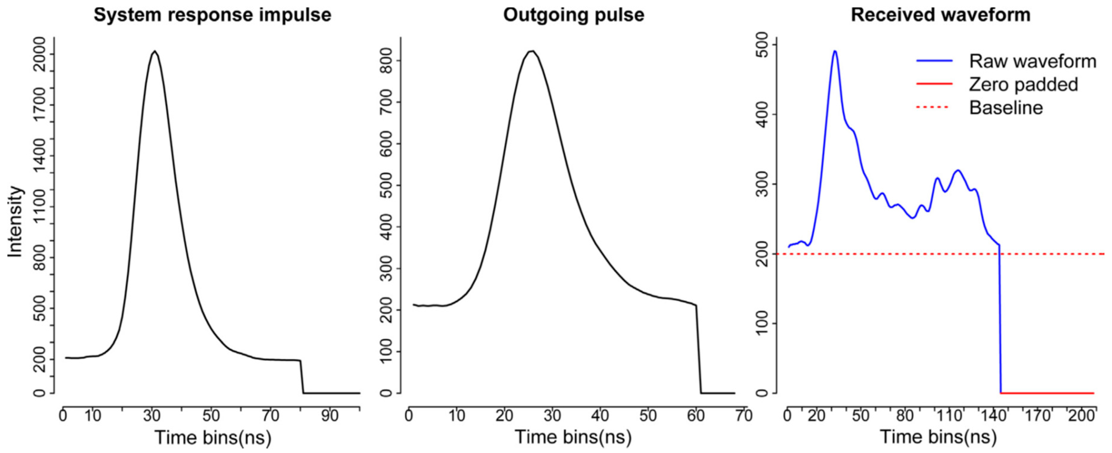
Compared to the decomposition, the deconvolution requires more input data and additional processing steps. Generally, we should have three kinds of data as the input for the deconvolution—the return waveform (RW), corresponding outgoing pulse (OUT) and the system response impulse (SRI) as shown in Figure 3 [6]. The RW and OUT are directly provided by the vendor. Ideally, the SRI is obtained through the calibration process in the lab before the waveform data are collected. In our case, NEON provided a return impulse response (RIR) which can be assumed as a prototype SRI. This system impulse was obtained through a return pulse of single laser shot from a hard ground target with a mirror angle close to nadir. Meanwhile, NEON also provided the corresponding outgoing pulse of this return impulse response (RIR_OUT). The “true” system impulse response can be obtained by deconvolving the RIR_OUT.

In this package, we provide two options for users to deal with the system impulse response (SRI). One is directly to assume the RIR as the SRI by assigning imp = RIR. Another is to obtain the SRI through deconvolving the OUT_RIR. In the function, the “true” SRI can be achieved by assigning imp = RIR and imp_out = OUT_RIR.

Two algorithms including the RL and Gold algorithms are available for the deconvolution. There are three main parameters for the deconvolution algorithms—(1) iterations: Number of iterations between boosting operations; (2) repetitions: The number of repetitions of boosting operations, which must be greater or equal to one; the total number of iterations is repetitions*iteration; and (3) boosting coefficient/exponent—the exponentiation of iterated value. These parameters will be valid only if repetition is greater than one and its recommended range is [1,2]. Our experiments showed that the boosting had less impact on the deconvolution results than the other two parameters. The value of 1.8 was assigned for the default boosting coefficients. The number of iterations and repetitions were critical to the performance of the deconvolution, which requires us to conduct the optimization process. One way of conducting the optimization process had been described in our previous study [6]. Moreover, the complexity of the waveforms generally required larger number of iterations and repetitions, which spurred us to add two arguments (large_paras and small_paras) for assigning suitable deconvolution parameters based on the number of waveform components (nwc). The np is an integer as the threshold parameter for determining using the large_paras (nwc > a anp) or small_paras (nwc <= np). For each argument, there are six parameters including the iterations, repetitions and boost parameters for deconvolving the SRI and the OUT.

data(return); data(outg); data(imp)  ##The impulse function is generally one for the whole study area

data(imp_out)

re<-return[1,]; out<-outg[1,]; imp<-imp; imp_out<-imp_out

option1: to obtain “true” system impulse response using the return impulse response (imp) and corresponding outgoing pulse (imp_out)

gold0<-deconvolution(re = re,out = out,imp = imp,imp_out = imp_out)

rl0<-deconvolution(re = re,out = out,imp = imp,imp_out = imp_out,method = “RL”)

option2: assume the provisional return impulse response RIP is the system impulse response (SRI)

gold1<-deconvolution(re = re,out = out,imp = imp)

rl1<-deconvolution(re = re,out = out,imp = imp,method=“RL”,small_paras = c(30,2,1.5,30,2,2))

After obtaining the deconvolution results, we can employ the peakfind, decom or decom.adaptive functions to get the possible objects’ corresponding time locations (µ) and other related parameters (A and σ). The time location information will be used for the subsequent geolocation transformation to generate the waveform-based point cloud. Other parameters can be appended to the point cloud and provide additional information for vegetation characterization.

To exemplify differences of our waveform processing methods, we selected three waveform examples to demonstrate results of decomposition and deconvolution methods in Figure 4. The detailed description of these methods has been reported in Zhou et al. [6].

3.2.5. Geolocation Transformation

This function is primarily used to transform waveforms into point clouds based on the decomposition results and reference geolocation data. The reference geolocation data were generally coming with the return waveforms and provided by the data vendor. Generally, reference geolocation data include original x, y, z reference information (orix, oriy, oriz) and the position change for x, y, z direction (dx, dy, dz) per time unit (ns). In addition, we also need to know the first return reference bin location (refbin) for the decomposition results. For the deconvolution results, the time of peak location for each outgoing pulse (outp) and the time of corresponding reference bin location for the outgoing pulse (outref) is also needed. Detailed description of the data and steps for calculation were given in Zhou et al. [14].

Our package provided one function named geotransform to quickly integrate decomposition result with reference geolocation data (geo) to generate points with relevant information. For the geo, we need to assign specific names to each column, which were used to calculate the absolute position of the time location in the waveform. To optimize the calculation process, we need to rename column names of geo-reference data, which is critical to the successful implementation of the function.

data(geo)  ### the reference geolocation

geoindex<- c(1:9,16)

colnames(geo)[geoindex]<-c(“index”,”orix”,”oriy”,”oriz”,”dx”,”dy”,”dz”,”outref”,”refbin”,”outpeak”)

decomre<-geotransform(decomp=rpars,geo)

Of particular note, the caution should be exercised in using this function. Because the geo-reference data format and their corresponding relationship with waveform data may vary for different data vendors, which require users to explore the corresponding relationship for subsequent calculation.

3.2.6. Waveform Variables

In addition to classical methods such as the decomposition and deconvolution (Method 1), we also explored another way (Method 2) to decode information inherent in waveform through directly extracting waveform metrics or signatures from waveforms. Unlike the classical methods, waveform metrics or signatures are directly obtained from waveforms instead of point cloud after decomposition.

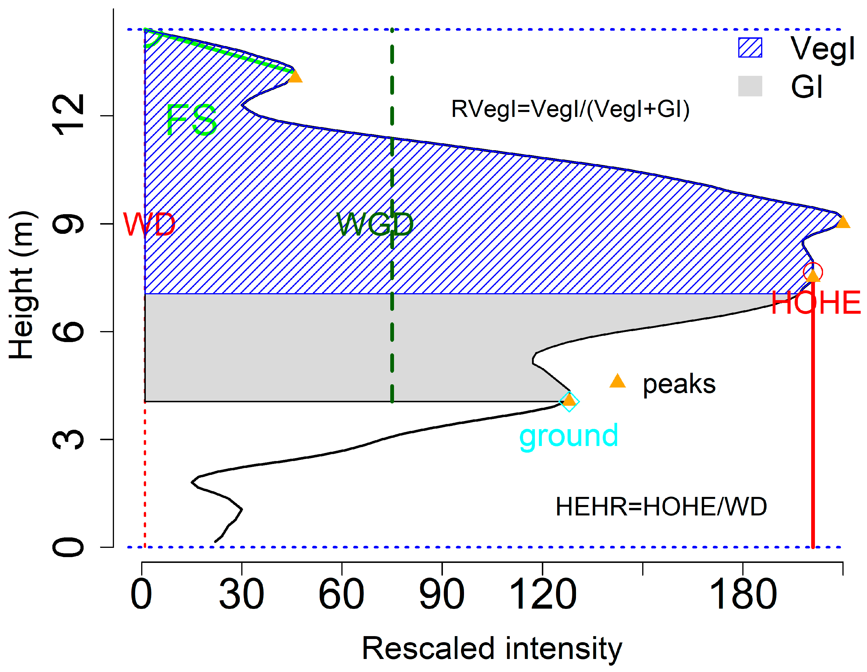
Our package provides some functions to obtain waveform metrics or signatures such as the height of median energy, front slope angle and the energy ratio between ground and vegetation from the waveforms for serving purposes of the Method 2. For example, the fslope function can help calculate the angle from waveform beginning to the first peak (front slope angle, FS) and the distance from the waveform beginning to the first peak (ROUGH), both of which can be used to differentiate the tree species in terms of crown structure. In addition, several intensity related functions such as percentiles can easily get the intensity-based characteristic from the waveforms. For example, we can calculate the intensity percentiles [0.45, 0.5, 0.55, …, 0.95] with percentile.location function and obtain the relative time location of these percentiles.

data(return); x<-return[182,]; qr<-seq(0.45,0.99,0.05); re<- percentile.location(x)

With these time locations, we can calculate the relative height of these percentiles. We assumed that the relative height is the height between the given location to the end of the waveform. To calculate the relative height of these intensity percentiles, we need to assign top = FALSE to make the intensity percentiles and the ground location index start at the end of the waveform. Another factor we need to know for calculating the relative height is the temporal resolution of a waveform. Here, our waveform was digitized with 1 ns temporal resolution which is approximately 0.15 m.

re1<-percentile.location(x,quan=qr,top=FALSE)

rh1<- (re1-ground.location(x,top = FALSE))*0.15

wd<- wavelen(x)*0.15

wgd<- (wavelen(x) - ground.location(x,top = FALSE))*0.15

num_peaks<- npeaks(x)

In this example, there is no negative value for rh1 since multiple waveform peaks are observed for this waveform. The negative values of relative height represent these locations are below the assumed ground level and caution should be exercised in real applications. Another important function is to obtain the integral (the area under the waveform curve) of assumed vegetation and ground with the integral function. You also can choose to use the raw waveform intensity by assigning rescale = FALSE to conduct the integral calculation. But using the minimum intensity (baseline) to conduct rescaling generally make more sense for generating integral related parameters.

xx<-return[182,]

rr1<-integral(xx)

To demonstrate the waveform metrics derived from waveform, we plotted several of them in Figure 5. Detailed description of these variables can be found in Zhou et al. [11]. Certainly, there are more variables can be generated from the waveform based on the users’ purposes.

These functions were mainly oriented for one waveform. Some researchers or users may be more interested in the waveforms within one specific region or given extent. The waveformclip function was designed to meet this requirement. For example, we can select waveforms within the region of interest by specifying the geo-extent or a shapefile. It is worthy to note that the shapefile should have the same projected coordinate system with the geo dataset.

data(geo); colnames(geo)[2:9]<-c(“x”,”y”,”z”,”dx”,”dy”,”dz”,”or”,”fr”)

data(return); waveform<-data.table(index=c(1:nrow(return)),return)

shp<-shp_hf; swre<-waveformclip(waveform,geo,shp)

swre1<-waveformclip(waveform, geo, geoextent=c(731126,731128,4712678,4712698))

Once a user has selected the waveforms within the region of interest (ROI), the functions used above can be applied to these waveforms to obtain results up to users’ purposes. In addition, a user also can combine theses waveform into one waveform and then process this waveform to obtain the characteristic of objects within the ROI.

3.2.7. From Waveforms to Hyper Point Cloud

To enrich existing waveform processing methods and reduce technical barriers of extracting useful information from FW LiDAR data, we developed a new way to process FW LiDAR data by converting all waveform intensities into points to form a very large point cloud dataset. The concept of this method is illustrated in Figure 6 [14] by combing raw waveforms with corresponding reference geolocation information. The notable feature of the point cloud in Figure 6b is the high density with ~177 points/m² (ppm²) that preserves as much information embed in the original waveforms. Additionally, its point cloud format can be easily adopted by most potential users using existing LiDAR tools or software such as LAStools and FUSION. The point cloud converted from FW LiDAR is much denser than the corresponding discrete-return LiDAR data (~7 ppm²). Consequently, we named this product the HPC. Detailed conversion steps and their potential applications can be found in Zhou et al. [14].

The following example shows how we generate the HPC with the hyperpointcloud function. To generate the HPC, we need to prepare two input datasets, the waveform data and corresponding geo-reference data. Before running this function, we need to check the geo-reference data and assign column names to them. This step is critical for the subsequent calculation which requires us to give exactly the same column names as follows.

data(geo); data(return)

geo$index<-NULL; colnames(geo)[1:8]<-c(“x”,”y”,”z”,”dx”,”dy”,”dz”,”or”,”fr”)

hpc<-hyperpointcloud(waveform=return,geo=geo)

For a large region, the computation of the hyperpointcloud function demands high RAM and volume of disk or memory storage. One solution is to divide waveforms into several tiles and process tiles separately as we showed in the following example. Another solution will be to use the SprakR package to manage the large data sets.

re<-NULL; chunks=5

row_interval<- round(seq(1, nrow(return),length.out = chunks))

for (i in 1:(chunks-1)){

  swf<- return[row_interval[i]:(row_interval[i+1]-1)]

  sgeo<- geo[row_interval[i]:(row_interval[i+1]-1)]

  sre<- hyperpointcloud(swf,sgeo)

  fwrite (sre,paste0(“subset_hpc_”,i,”.csv”))}

It is noteworthy that there is no standard format of FW LiDAR data and the current version of the hyperpointcloud function may be only suitable for calculating the FW LiDAR data with similar format to the data (NEON) we exemplified. However, the concept and methods can be extended to other kinds of FW LiDAR data once the data structure and corresponding geo-reference data are given.

3.2.8. Waveformgrid

The HPC can relieve users’ concerns on the technical intricacy of waveform processing. However, not every point in the HPC are useful, which require us to conduct additional steps to generalize useful information from the HPC up to users’ purpose. We explored several potential applications of the HPC on vegetation characterization. One example is to apply a grid-net for the HPC to obtain the useful information the waveforms contained. There are two ways to generalize useful information from raw waveforms in the waveformgrid function—(1) using the HPC product as the input and summary the information in each grid cell users defined; (2) using the raw waveforms and corresponding geolocation reference data to obtain information within each grid cell. Unlike the first method, the principle of the second method is to select waveforms instead of to select points within each grid, which means we can still use the waveformgrid function without generating the HPC. Specifically, we assigned the geolocation (the middle point of the waveform) to each waveform based on the corresponding geo-reference data. Through this geolocation information, we can select potential waveforms in the grid and further derive candidate parameters such as the mean intensity and maximum intensity of the grid. The size of the grid is crucial for the 2D surface generation which requires users to experiment different sizes and optimize this parameter up to their purposes.

In the following example, we used both methods to generate waveform gridding results. Actually, there is no significant difference between these two methods when the grid size is small (<~2 m). However, the second method requires less computation and storage memory to obtain final results than the first method (the HPC method).

####using hpc as input, the first method

hpcgrid<-waveformgrid(hpc=hpc,res=c(1,1))

###using raw data as input, the second method

rawgrid<-waveformgrid(waveform = return, geo=geo, res=c(1,1),method=“Other”)

By default, there are four features calculated in each grid cell—the number of waveform signals, the maximum intensity, mean intensity and the minimum intensity. In addition, this function also provided an option to calculate the percentile intensity within the grid cell. To implement this step, we need to assign the quan argument, which are the percentiles you are interested in. In the following example, we calculate the intensity percentile c(0.4,0.48,0.58,0.67,0.75,0.85,0.95) within the grid using the HPC as the input.

quangrid<-waveformgrid(hpc=hpc, res=c(1,1),quan=c(0.4,0.48,0.58,0.67,0.75,0.85,0.95)

Results of quangrid not only include both four representative intensity, it also gives the percentile intensity based on the user-specified quantiles.

To generate a 2D surface, we converted cx, cy and one of these intensity variables to the point cloud as the LiDAR data exchange binary format (LAS) and generated the digital surface model (DSM) for each point cloud using the lasgrid function from LAStools [11]. Figure 7 [14] is an example of the discrete-return (DR)-based digital surface model (DSM) and (b) the HPC-based MAXI DSM, (c) HPC-based MI DSM and (d) HPC-based 99th percentile height (PH) DSM from the HPC. The visualization of these results is demonstrated in the Quick Terrain Modeler (QTM).

3.2.9. Waveformvoxel

Similar to the concept of the waveformgrid, our package also provided a 3D representation of the HPC using the waveformvoxel function. Through this function, the HPC data will be divided into 3D space to form multiple voxels (Figure 8d), which could give us more detailed information of the objects the waveforms interact with than the 2D projected products. Moreover, this method also paves a way for generalizing useful information from the HPC.

The principle behind the voxel is that the neighborhood points shared similar characteristics and the information within the homogenous unit can be represented by one quantity or one voxel. The following example shows how to voxelize data from the HPC. The main parameter of this function is the voxel size (res) which require you to assign a vector containing three values to represent voxel size in the X, Y and Z directions. Analogous to the waveformgrid, we also can generate the quantile intensity in each voxel by adding the quan argument.

voxr<-waveformvoxel(hpc,res=c(1,1,0.15))

qvoxr<-waveformvoxel(hpc,res=c(1,1,0.15),quan=c(0.4,0.5,0.75,0.86))

As shown in Figure 8, we conducted a comparison of an individual tree represented by the discrete-return LiDAR data (Figure 8a) and HPC related products. Specifically, Figure 8b shows the waveforms we cropped from the whole dataset using the waveformclip function. To directly visualize these waveforms, the hyperpointcloud function was used to convert these waveforms into the HPC as shown in Figure 8c. Compared to Figure 8a, the HPC has a larger height range with more points at the top of the canopy and the bottom of the group. Furthermore, we also present the HPC in a voxel format (Figure 8d) coloring by intensity through the waveformvoxel function. The size of the voxels is dx = 0.8, dy = 0.8 and dz = 0.15 m. It can be observed that the higher intensity is more likely to be located at the ground and the tree top area. While the mid-story of the tree is more likely to have lower intensity. The shape of the tree crown can be vaguely recognized from Figure 8d, however, a useful representation of individual trees with the HPC or voxels needs subsequent filtering and further removal of redundant information. As an example, we presented three voxelization trees after conducting intensity filtering with 60% (Figure 8e), 65% (Figure 8f) and 70% quantile (Figure 8g of intensity. As anticipated, fewer voxels are left to represent the vegetation structure with the increase of the intensity threshold. Interestingly, the crown shape and vegetation structure can be reconstructed to some extent using filtering voxels. Especially when we used 60% quantile of intensity to filter the voxels, the internal structure of the individual tree can be observed. Moreover, a simple filtering strategy was implemented at the current stage. With a comprehensive filtering, more representative voxels are expected. Undoubtedly, this will provide an insightful way to characterize vegetation structure using waveform LiDAR data.

3.2.10. Rawtocomposite

Most of the waveforms are not directly vertically distributed along the pulse line due to the fact that the outgoing pulse was emitted at an off-nadir angle as shown in Figure 8c,h. This off-nadir angle can enhance the capability of the laser to penetrate through gaps in the forest canopy but on the other hand, it also results in the negative effect on the vegetation structure characterization and data merging from multiple flight lines [11,15]. To mitigate this negative effect on the internal structure characterization, we developed a new way to generate vertical waveforms from the waveform voxelization results. The principle of this method is to reconstruct the raw waveforms from the products generated from the waveformvoxel function. The rawtocomposite function of our package can take these voxels as input and reconstruct waveforms without tilt angle (composite waveforms) based on the choice of voxel intensities (maximum, mean or percentile intensity). Subsequently, composite waveforms are treated as original waveforms and can recreate the HPC using the hyperpointcloud function. To better demonstrate results, we present a comparison of the original HPC (Figure 8h and composited waveform based HPC (Figure 8i after using 60% quantile intensity as the filter. We can see those points in Figure 8i are vertically distributed as compared to Figure 8h. In addition, we also compared the capability of composite waveforms with the original waveforms on vegetation characterization such as tree species identification [11]. The comparisons have shown that the composite waveform has an advantage over the raw waveform on the tree species identification. Certainly, more efforts are needed to further test its performance and facilitate its potential applications. Of particular note, the composite waveform needs additional processing steps and higher computation cost, which calls for cost-benefit analysis prior to large scale application using composite waveforms. The original waveforms may be sufficient to achieve the necessary accuracy of vegetation characterization under specific circumstances.

The following example gave us a snapshot of how to use the rawtocomposite function to obtain the composite waveforms. In addition, we provide an option to enable users to select which intensity variables they want to formulate in the composite waveform. By default, we used the maximum intensity (inten_index = 2) of each voxel to represent the intensities of the composite waveforms. In the second example, we assigned inten_index to 6 which represents we used the 50% percentile intensity to represent the intensity of the composite waveform. In this example (qvoxr), there are eight intensity related variables were generated—the number of intensities, the maximum intensity, the mean intensity, total intensity, 40th percentile intensity, 50th percentile intensity, 75th percentile intensity and 86 percentile intensity in each voxel. It is important to note that the resolution of composite waveform relied on the setting of the waveformvoxel function.

rtc<-rawtocomposite(voxr)

ph_rtc<-rawtocomposite(qvoxr,inten_index = 6)

4. Conclusions

The present paper aims to introduce the waveformlidar package and its applications to R users. We incorporated commonly used FW processing algorithms with a new development of FW LiDAR data analysis, which is expected to alleviate the technical barrier of exploring FW LiDAR data and give users more flexibility to interpret results. Multiple examples are presented to illustrate various features of the package. For example, several decomposition methods such as the Gaussian decomposition and Gold deconvolution are available for the ecological and remote sensing communities to implement sophisticated waveform processing algorithms in a comfortable way. In addition, we also demonstrate a new way to directly visualize the FW LiDAR data in terms of point cloud data structure and exemplify the potential usefulness of the HPC.

To date, only part of the functions available in waveformlidar are discussed in detail. More examples of FW LiDAR data applications can be found at https://github.com/tankwin08/waveformlidar. The package is still under continuous development and suggestions for further features can be submitted to https://github.com/tankwin08/waveformlidar/issues.