Article

Removal of Large-Scale Stripes Via Unidirectional Multiscale Decomposition

1
State Key Laboratory of Information Engineering in Surveying, Mapping and Remote Sensing (LIESMARS), Wuhan University, Wuhan 430079, China
2
School of Computer, Hubei University of Technology, Wuhan 430068, China
3
Collaborative Innovation Center of Geospatial Technology, 129 Luoyu Road, Wuhan 430079, China
4
School of Resource and Environment Sciences, Wuhan University, Wuhan 430079, China
*
Author to whom correspondence should be addressed.
Remote Sens. 2019, 11(21), 2472; https://doi.org/10.3390/rs11212472
Submission received: 28 August 2019 / Revised: 21 October 2019 / Accepted: 21 October 2019 / Published: 23 October 2019
(This article belongs to the Special Issue Quality Improvement of Remote Sensing Images)

Abstract

:
Stripes are common in remote sensing imaging systems equipped with multichannel time delay integration charge-coupled devices (TDI CCDs) and have different scale characteristics depending on their causes. Large-scale stripes appearing between channels are difficult to process by most current methods. The framework of column-by-column nonuniformity correction (CCNUC) is introduced to eliminate large-scale stripes. However, the worst problem of CCNUC is the unavoidable cumulative error, which will cause an overall color cast. To eliminate large-scale stripes and suppress the cumulative error, we proposed a destriping method via unidirectional multiscale decomposition (DUMD). The striped image was decomposed by constructing a unidirectional pyramid and making difference maps layer by layer. The highest layer of the pyramid was processed by CCNUC to eliminate large-scale stripes, and multiple cumulative error suppression measures were performed to reduce overall color cast. The difference maps of the pyramid were processed by a designed filter to eliminate small-scale stripes. Experiments showed that DUMD had good destriping performance and was robust with respect to different terrains.

Graphical Abstract

1. Introduction

High-resolution optical remote sensing satellites are generally imaged by time delay integration charge-coupled devices (TDI CCD) sensors. A single CCD consists of multiple taps, and different taps have different levels of circuit noise. Moreover, a camera is often spliced by multiple CCDs to satisfy image width requirements. Therefore, a single linear camera has multiple channels. With a single channel, there is high-frequency response nonuniformity between different detectors, and this nonuniformity will produce small-scale stripes. With multiple channels, there is low-frequency response nonuniformity, which will produce large-scale stripes [1]. For example, the optical satellite Gaofen-1B (GF-1B) is equipped with two multispectral cameras, each camera has three CCDs, and each CCD has two taps. That is, a GF-1B multispectral image forms 12 channels. If the nonuniformity is not effectively corrected, the large-scale stripes will exist between these channels, and the small-scale stripes will exist in these channels.
Before and after the launch of a satellite, the staff will perform laboratory and on-orbit relative radiation calibration for the sensors to eliminate nonuniformity. However, errors can occur in the process of relative radiometric calibration, and the radiation response of the detectors will drift with time [2]. Given these and other random factors, some remote sensing images (especially medium- and long-wave infrared images) will still contain stripes [3]. This characteristic will adversely affect image quality and subsequent use.
Current destriping algorithms can be mainly divided into filtering-based methods, statistical-based methods, and variation-based methods. Filtering-based methods are the earliest proposed destriping algorithms and include space-frequency domain filtering and wavelet domain filtering [4,5,6,7,8,9]. Space-frequency domain filtering methods treat stripe noise as periodic noise and use a low-pass filter to remove corresponding components [5]. Wavelet domain filtering methods mainly utilize the directionality of stripe noise and the sensitivity of wavelet to the direction [6]. Stripe noise is removed by processing the wavelet coefficients. Filtering-based methods have simple calculations and are easy to implement. However, the real signal and the noise signal cannot be separated, resulting in the loss of image detail and making the destriped image fuzzy.
To overcome the blurred effect of filtering-based methods, scholars have gradually turned to statistical-based methods. Statistical-based methods include histogram matching [10], moment matching (MM) [11], and its improved versions (IMM) [12,13]. Statistical-based methods all have certain assumptions and are limited by image size, terrain distribution, and other conditions. Histogram matching assumes that the histogram of each column in the image has the same distribution. Moment matching assumes that the standard deviation and mean value of each column in the image are the same. If the image size is too small or the terrain difference is too large, these statistical-based methods cannot achieve satisfactory results. The destriping effect of statistical-based methods depends on the universality and rationality of their assumptions. Since the assumption of moment matching is more general, its processing effect will be better than histogram matching.
The general pattern of variation-based methods is to construct the relationship model between stripe noise and real signal and eliminate the stripe by minimizing the model function [14,15,16,17]. The key issue is how to analyze and construct a suitable model. The total variation (TV) was firstly introduced by Shen in destriping because of its great edge retention ability [14]. Since then, scholars have proposed a variety of improvements. Boual [15] proposed the unidirectional TV (UTV) model, which assumed that the gradient in the vertical direction of the stripes is not affected. Based on UTV, Zhou [16] proposed the spatially adaptive unidirectional total variation (SAUTV) model, which improved robustness and edge retention ability. The variation-based methods approach works well, but the calculations are complex, and the performance is extremely dependent on the choice of parameters.
Stripes have different scales due to their different causes. For large-scale stripes between channels, most current methods have difficulty achieving satisfactory results. To solve this problem, this paper proposed a destriping method based on unidirectional multiscale decomposition (DUMD). A stripe image was decomposed by constructing a unidirectional pyramid and making difference maps layer by layer. The large-scale stripes and small-scale stripes were separated by multiscale decomposition. The large-scale stripes were contained in the highest layer of the pyramid and eliminated by column-by-column nonuniformity correction (CCNUC). The small-scale stripes were contained in difference maps and eliminated by a designed filter. The algorithm was tested with six sets of simulation data, and the results were compared with MM, IMM, and SAUTV. Experiments showed that the DUMD algorithm had good performances, could remove stripes with different scales, and was robust to terrain differences.
The remaining parts of this paper are as follows. Section 2 analyzes the causes and characteristics of stripe noise. Section 3 describes the specific method of the DUMD algorithm. Section 4 describes and analyzes the experimental results. Section 5 summarizes this paper.

2. Analysis of Stripe Noise

2.1. Conversion of the Destriping Problem

The no-stripe image is denoted L , the striped image is denoted L * , the destriped image is denoted L ^ . Assuming that they are all of the size M × N , and that L * is affected by multiplicative and additive stripe noise simultaneously,
p i , j * = k j × p i , j + b j
where p i , j * is the pixel in L * , p i , j is the pixel in L , k j is the multiplicative stripe noise of the j th detector, b j is the additive stripe noise of the j th detector, and subscripts i , j are the row and column indexes, respectively.
The j th column of L is denoted P j = [ p 1 , j , p 2 , j , , p M , j ] T , the mean value of P j is denoted a j , and the standard deviation of P j is denoted s j . Similarly, the j th column of L * is denoted P j * = [ p 1 , j * , p 2 , j * , , p M , j * ] T , the mean value of P j * is denoted a j * , and the standard deviation of P j * is denoted s j * . These values have the following relationship:
{ a j * = k j a j + b j s j * = k j s j
It can be seen from Equation (2) that standard deviation is only affected by the multiplicative noise, while the mean value is affected by both multiplicative and additive noise. For the j th column, the stripe noise can be eliminated if a j and s j can be determined. Moment matching assumes that a j and s j equal the mean and standard deviation of the overall image. The performance of moment matching depends on the image size and terrain uniformity of the imaged area. If the image size is too small or the terrain is not sufficiently uniform, moment matching will produce new stripes.
If the additive noise is ignored, then the destriped pixel can be expressed as:
p ^ i , j = p i , j * k ^ j = p i , j + b j ( a j p i , j ) k j a j + b j
where p ^ i , j is a pixel in L ^ and k ^ j = a j * / a j is the approximate multiplicative noise. It can be seen from Equation (3) that if the additive noise is ignored, there will be an error term whose value is equal to b j ( a j p i , j ) k j a j + b j .
Multiplicative noise is the main component of stripes; its main sources are the nonuniformity of responses, the gain amplification effect, and other factors. Additive noise is the secondary component of stripes; its main source is dark current whose intensity is relatively small. The error term caused by ignoring additive noise is relatively small. If the mean value of every column can be obtained, the no-stripe image can be reconstructed. The mean values of the columns can be written as a vector (the column mean vector, CMV). Therefore, the destriping problem can be transformed into estimating the optimal CMV of the no-stripe image.

2.2. Scale Characteristics of Stripes

Stripes have different scale characteristics depending on their sources. For a single channel (tap), the sources of the stripes include photo shot noise, reset noise, dark current, fixed pattern noise, and quantization noise [18,19]. The stripes in the channel appear as thin lines in the image and appear as small-scale impulse noise on the corresponding CMV. Figure 1a shows the Band4 of GF-1C as an example of small-scale stripes, and Figure 1c is its corresponding CMV.
The optical sensor in the satellite is generally formed by multiple CCDs, and each CCD is formed by multiple taps, causing a linear camera to have multiple channels. Different channels have different circuit noise, and the circuit noise is amplified by the gain, which causes the image to produce an obvious color cast. Stripes between channels are large-scale and of high-intensity and appear as large-scale steps in the corresponding CMV. Figure 1b shows the Band2 of GF-2 as an example of large-scale stripes, and Figure 1d is its corresponding CMV. This large-scale stripe appears at the junction of two CCDs. It is caused by the nonuniformity of the two CCDs, and this nonuniformity is not repaired by radiometric correction completely.
Small-scale stripes are easy to process, either by filtering the CMV or by using some variation-based methods. However, it is difficult to process large-scale stripes. To eliminate large-scale stripes, we introduced the framework of column-by-column nonuniformity correction (CCNUC), which is based on the spatial similarity of remote sensing images.

3. Methodology

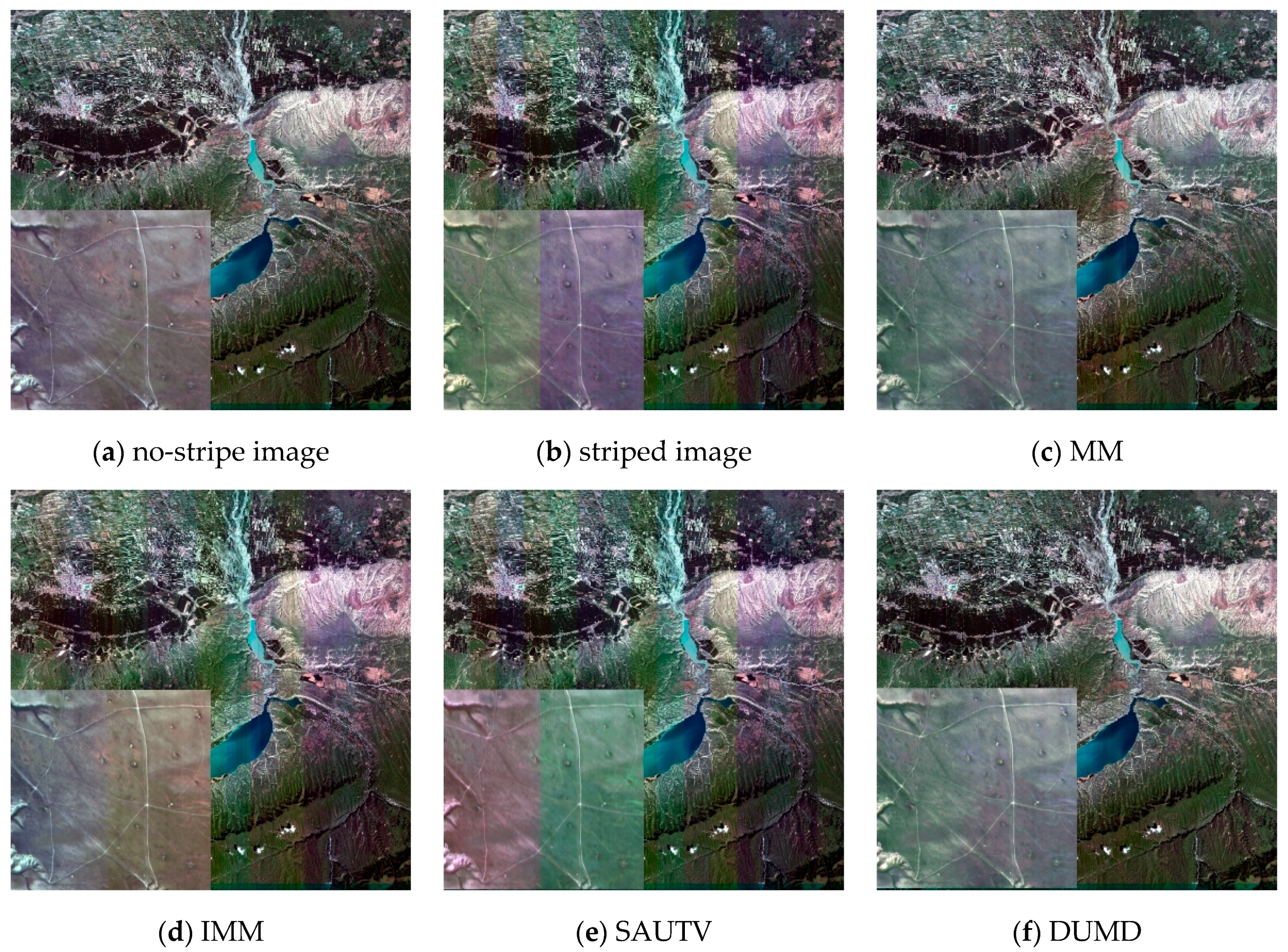
3.1. Overall Description of DUMD

When establishing the unidirectional pyramid of stripe image L * { L 0 * , L 1 * , , L n * } , the large-scale stripes are saved in the highest layer L n * , and the small-scale stripes are saved in difference maps. The difference map of the i th layer is written as D i * and is defined as:
D i * = L i * L i + 1 * , ( i = 0 , 1 , , n 1 )
where L i * and L i + 1 * both need to be resampled to have the same size as L * . The CMVs of { L 0 * , L 1 * , , L n * } are denoted { A 0 * , A 1 * , , A n * } , and the corresponding destriped CMVs are denoted { A ^ 0 , A ^ 1 , , A ^ n } , respectively. The CMVs of { D 0 * , D 1 * , , D n 1 * } are denoted { E 0 * , E 1 * , , E n 1 * } , and the corresponding destriped CMVs are denoted { E ^ 0 , E ^ 1 , , E ^ n 1 } , respectively. Extending Equation (4), we obtained:
E i * = A i * A i + 1 * , ( i = 0 , 1 , , n 1 )
Equation (5) illustrates that E i * can be obtained from A i * and A i + 1 * and does not have to use D i * . Moreover, A i * can be obtained from the downsampling of A * (the CMV of L * ) and does not have to use L i * . Therefore, only A * needs to be calculated from two-dimensional data, while the other CMVs ( A i * , E i * ) are all calculated from one-dimensional data; this feature can greatly reduce the amount of calculation.
In Section 2.1, the destriping problem was converted into the CMV estimation of the no-stripe image. Therefore, the destriped image L ^ can be expressed as:
L ^ = L * × A ^ A * A ^ = Α ^ n + i = 0 n 1 E ^ i
In Equation (6), the destriping problem has been converted into the problem of seeking Α ^ n and E ^ i . The small-scale stripes are saved in D i * , which is eliminated by E ^ i . Small-scale stripes are easy to process, and we have designed a filter G ( ) to remove them. Assuming E i * = [ e i , 1 * , e i , 2 * , , e i , N * ] and E i = E i * h 1 d = [ e i , 1 , e i , 2 , , e i , N ] (where h 1 d is a one-dimensional smooth kernel), the filter can be expressed as:
E ^ i = G ( E i * ) = { e i , j   , i f   | e i , j * e i , j | > δ e i , j *   , i f   | e i , j * e i , j | δ
where δ is a threshold used to judge small-scale stripe noise; δ was set at 1 in this paper.
The large-scale stripes are saved in L n * , which is eliminated by Α ^ n . Large-scale stripes are difficult to process; this difficulty was the main issue addressed in this paper. The CCNUC framework was applied to obtain A ^ ; this process has been described more thoroughly in Section 3.2. However, the cumulative error produced by CCNUC cannot be ignored, and additional measures must be applied for suppression. These cumulative error suppression measures are described in Section 3.3, Section 3.4 and Section 3.5.
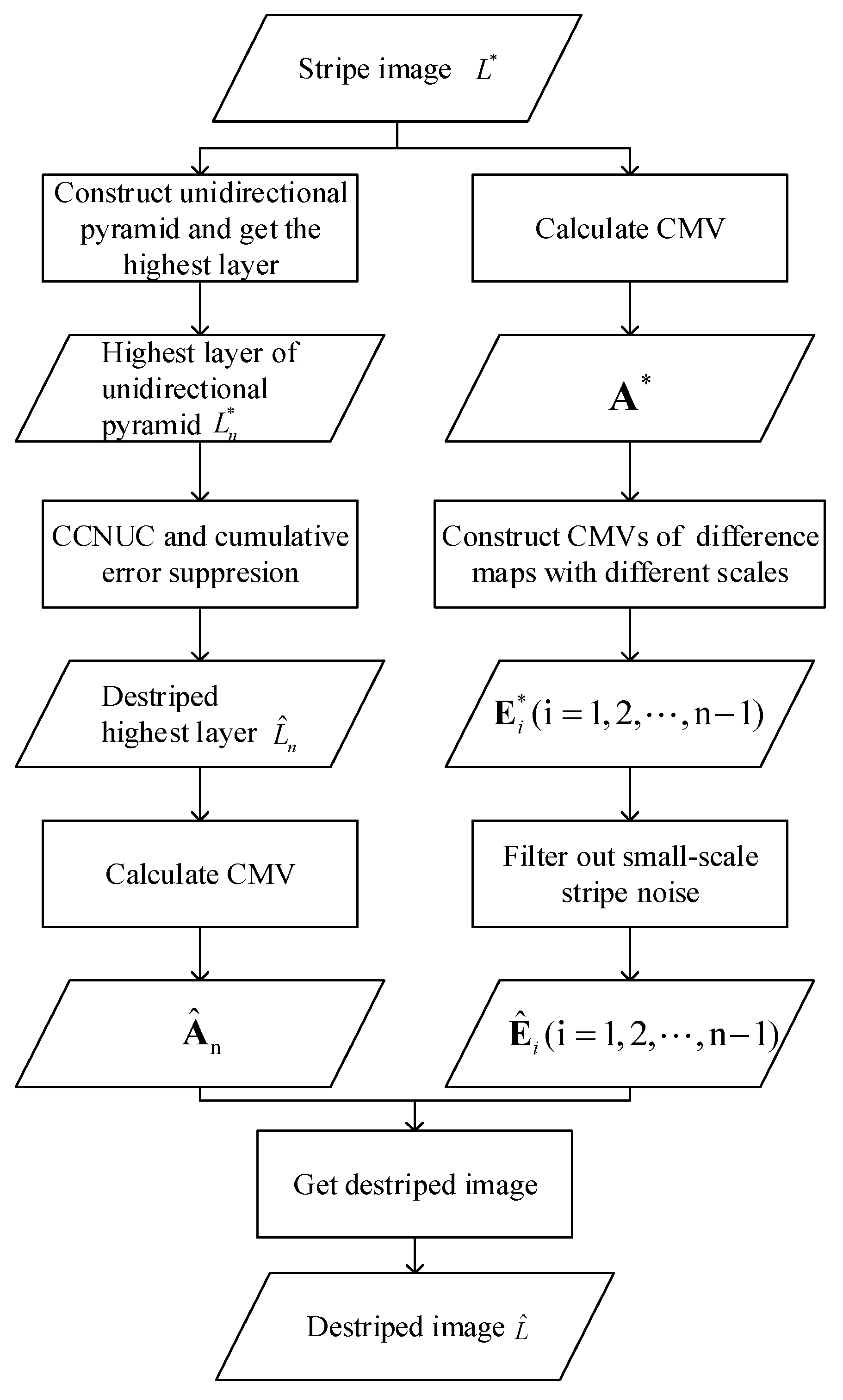
In summary, the overall process of the DUMD algorithm is shown in Figure 2, and mainly includes five steps:
(1) A unidirectional pyramid of the stripe image is constructed, and the highest layer L n * is obtained.
(2) CCNUC and cumulative error suppression measures are performed on L n * to obtain the destriped layer L ^ n and the corresponding CMV Α ^ n .
(3) In accordance with Equation (5), { E 0 * , E 1 * , , E n 1 * } are obtained by resampling and difference.
(4) In accordance with Equation (7), { E ^ 0 , E ^ 1 , , E ^ n 1 } are obtained by removing small-scale stripes.
(5) In accordance with Equation (6), the final destriped image is obtained by combining A * , Α ^ n , and { E ^ 0 , E ^ 1 , , E ^ n 1 } .

3.2. The Framework of Column-by-Column Nonuniformity Correction (CCNUC)

Remote sensing images have spatial similarity, and any two random adjacent columns should have similar statistical characteristics. Because of this feature, the stripe image can be corrected by CCNUC with various methods. In Section 2.1, the destriping problem was converted into the problem of estimating the CMV of the no-stripe image, so the stripe noise can be removed by calculating the deviation between adjacent columns. The CCNUC framework can be expressed as:
P ^ j = a 1 * + k = 2 j c k a j * P j * c k = F ( P k * , P k 1 * )
where P ^ j is the j th column of the destriped image, c k is the adjustment coefficient between P k * and P k 1 * , and F : ( X , Y ) c is a function that calculates the adjustment coefficient between two columns. The adjustment coefficient c k can be divided into two parts: the accurate part (denoted γ k ) and the error term (denoted ε k ). There is a cumulative error Δ between the estimated column P ^ j and the real column P j :
Δ = P ^ j P j = P j * a j * k = 2 j ε k
In Equation (9), the role of P j * a j * is to normalize P j * . Therefore, the intensity of Δ is positively correlated with the number of accumulations j and the magnitude of the single adjustment error ε k .
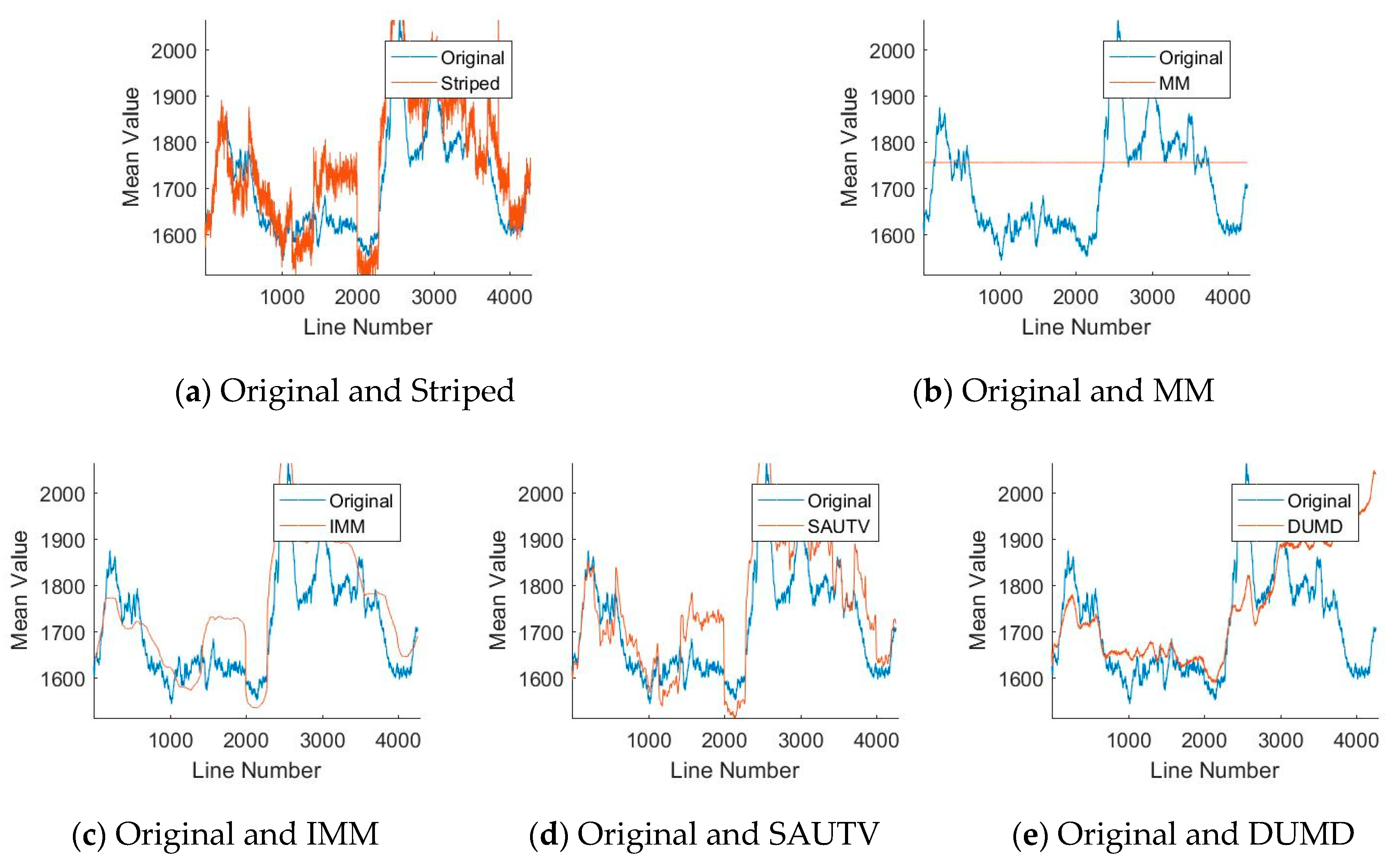
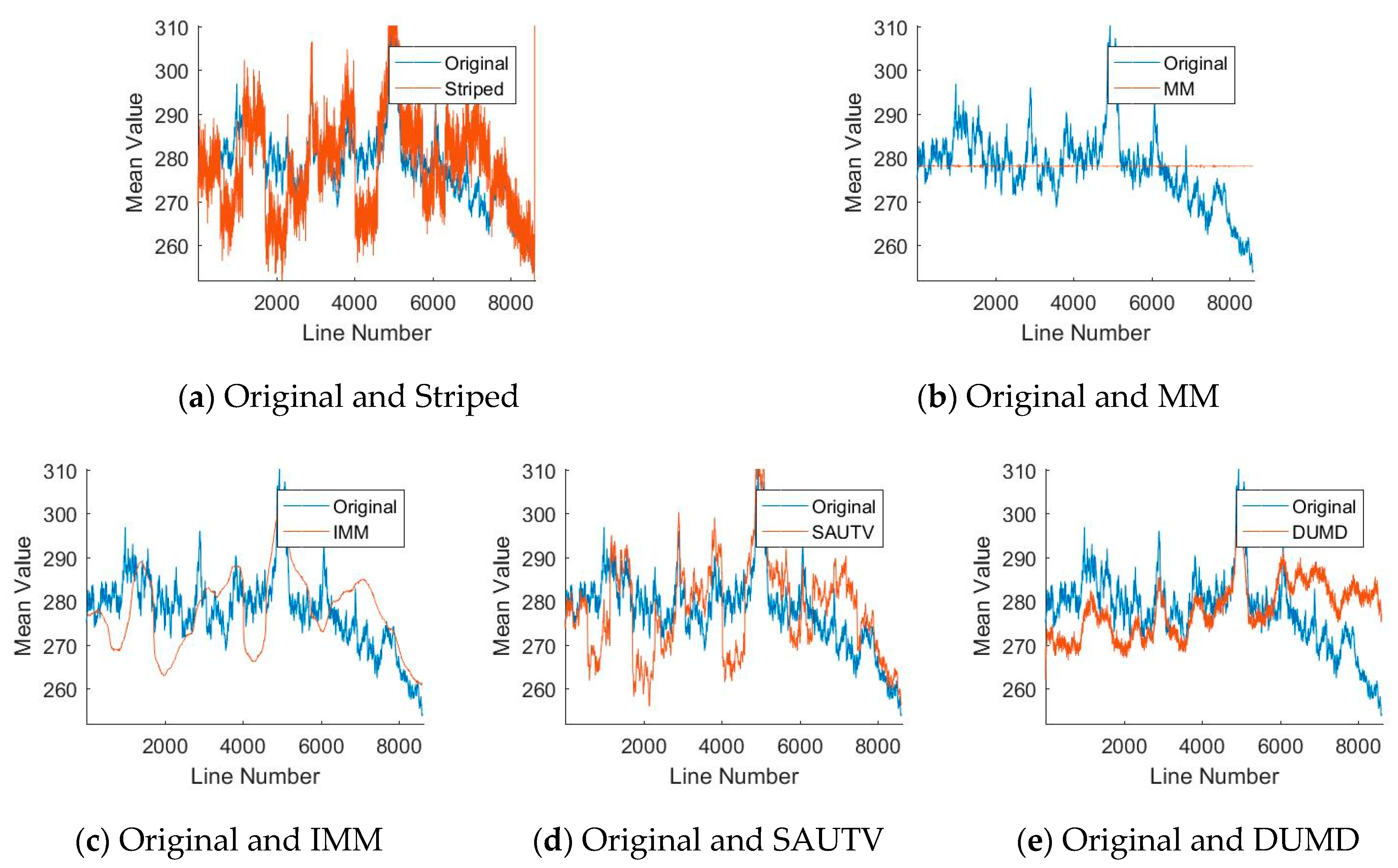
The cumulative error is an unavoidable problem of the CCNUC framework. In the image, the cumulative error appears as a color cast on the destriped image. The farther the error is from the initial column, the more serious the color cast. In the CMV, the cumulative error appears as an overall offset. The farther the error is from the initial point, the larger the offset. There are three steps that can be taken to compensate for the cumulative error produced by CCNUC:
(1) Reduce the number of error accumulations. By Equation (9), the intensity of Δ is positively correlated with j . Reducing the size of j is the most effective way to suppress the cumulative error. When the unidirectional pyramid of stripe image L * { L 0 * , L 1 * , , L n * } is established, only the highest layer L n * is processed by CCNUC. In this way, the cumulative number can be reduced from N 1 to N 2 n 1 . This step has been described in more detail in Section 3.3.
(2) Improve the accuracy of the single deviation estimation of adjacent columns (i.e., reduce the value of the single adjustment error ε k ). The cumulative error comes from the accumulation of multiple tiny errors, so improving the accuracy of every deviation estimation is also an effective suppression method. The size of ε k is related to the samples and the calculation method. The least-square method (LSM) is the most common method for calculating the linear relationship between two samples. However, its objective function is the root mean square error (RMSE), which is sensitive to extreme values (gross errors). If these extreme values cannot be excluded, the deviation estimation of the adjacent columns will be enlarged. Therefore, we proposed a deviation estimation method based on a normal distribution. This method can reduce the influence of extreme values and improve accuracy. This step has been described in more detail in Section 3.4.
(3) Design a compensation measure for cumulative error. The adjustment error ε k cannot be measured, but it has the property of accumulation. Using this property, we could detect it on a larger scale and compensate for it. Recording the initial corrected L n * as L ^ n ( 1 ) , decomposing L ^ n ( 1 ) to a larger scale, and making the second adjustment by the same method will compensate for cumulative error to some extent. This step has been described in more detail in Section 3.5.

3.3. Unidirectional Multiscale Decomposition

Because of their different causes, stripes have different scales. The stripes in the channel are small-scale and of low-intensity, and the stripes between channels are large-scale and of high-intensity. The unidirectional pyramid of stripe image L * { L 0 * , L 1 * , , L n * } is established by mean filtering with a filter size 1 × 3. All layers of the pyramid are resampled to the same size, and the difference maps are obtained by Equation (4). Then, the stripe image can be decomposed into the multiscale sets L * { D 0 * , D 1 * , , D n 1 * , L n * } .
Each layer of the unidirectional pyramid can only contain stripes of the same scale or larger scale. Therefore, each layer of the multiscale sets can only retain stripes of the same scale. In other words, stripes are completely decomposed into multiscale sets without overlap; L n * retains large-scale stripes, and D 0 * , D 1 * , , D n 1 * retain small-scale stripes.
Stripes appear as two-dimensional signals in the image, but they can be completely and losslessly compressed into one-dimensional signals in the corresponding CMV. Similarly, the CMVs of D 0 * , D 1 * , , D n 1 * ( E ^ 0 , E ^ 1 , , E ^ n 1 ) retain all the small-scale stripes, and the CMV of L n * ( A n * ) retains all the large-scale stripes. Small-scale stripes can be eliminated by filtering E ^ 0 , E ^ 1 , , E ^ n 1 . Therefore, only L n * needs to be processed by CCNUC; this processing can reduce the error accumulation number from the original N 1 to the current N 2 n 1 .
In the CCNUC framework, the adjustment parameter c k is calculated by the statistical characteristics of the adjacent columns. The availability of the statistical characteristics depends on the number of samples. If the image is shrunk by the same factor in width and length, then the number of pixels in each column will be drastically reduced, and the reliability of the statistical characteristics cannot be guaranteed. Therefore, it is only necessary to shrink the image in a single direction (perpendicular to the stripe direction) in the process of establishing the pyramid.

3.4. Deviation Estimation of Adjacent Columns

The actual features of the remote sensing image change gradually, indicating that the remote sensing images have a spatial similarity. Therefore, the premise of the CCNUC framework is that two adjacent columns in the remote sensing image should have similar statistical characteristics. When the statistical characteristics of adjacent columns have large differences, it indicates that there are external factors causing systematic radiation deviation (e.g., existing stripe noise). The key issue of the CCNUC framework is how to measure the statistical characteristics of adjacent columns. If the mean and standard deviation are used as statistical indicators, CCNUC is equal to moment matching. If only the mean is used as a statistical indicator, CCNUC is equal to simplified moment matching, and its performance will be worse.
Stripe noise will cause a linear change in the columns. LSM is the most popular method for calculating the linear relationship between two sets of samples. Although the adjacent columns have similarities, they are not identical. There are a few differences between adjacent columns. These differences are caused by features and are especially noticeable in the high-gradient region. The object function of LSM is the RMSE of the two sets of samples, and this RMSE is susceptible to extreme values. Therefore, using LSM to estimate the deviation between adjacent columns will cause over-estimation (i.e., will increase the absolute value of ε k ) and enlarge the cumulative error. Based on this consideration, this paper proposed a deviation estimation method based on the normal distribution, which could reduce the influence of extreme values and improve the robustness of the measurement.
If the radiation responses of two adjacent detectors are consistent, then the difference between the adjacent columns of their images can be considered to be caused by features. In this situation, the difference between the two adjacent columns should satisfy the zero-mean normal distribution:
X k N ( μ k , σ 2 ) ,   μ k = 0
where X k is the difference between adjacent columns, μ k is the mean of the normal distribution, which is equal to 0, and σ 2 is the variance of the normal distribution. If the radiation responses of two adjacent detectors are inconsistent, the fitting Gaussian curve will shift and μ k 0 . Therefore, the adjustment parameter can be obtained by measuring the mean of the Gaussian fitting curve of X k :
F ( P k * , P k 1 * ) = { μ k i f   | μ k | > η 0 i f   | μ k | η
where F ( ) is a function that calculates the adjustment parameter, P k * and P k 1 * are two adjacent columns, and η is the threshold introduced to reduce the algorithm error; it was set to the median of { μ 2 , μ 3 , μ N } in this paper.

3.5. Cumulative Error Compensation

After L n * has been processed by CCNUC once, the large-scale stripes have been filtered out. At this time, the initial destriped image L ^ n ( 1 ) retains the true information and the cumulative error. The cumulative error is the accumulation of the adjustment error in space. The single adjustment error ε k cannot be measured, but it has the property of accumulation. Three columns of L ^ n ( 1 ) are denoted P ^ k ( 1 ) , P ^ k 1 ( 1 ) , and P ^ k d ( 1 ) , where d > 1 . For P ^ k ( 1 ) and P ^ k 1 ( 1 ) , the result of F ( P ^ k ( 1 ) , P ^ k 1 ( 1 ) ) is completely untrustworthy. However, for P ^ k ( 1 ) and P ^ k d ( 1 ) , the result of F ( P ^ k ( 1 ) , P ^ k d ( 1 ) ) has a certain degree of confidence due to the cumulative nature of the error.
The value of F ( P ^ k ( 1 ) , P ^ k d ( 1 ) ) contains two parts: the difference in features and the cumulative error. Therefore, F ( P ^ k ( 1 ) , P ^ k d ( 1 ) ) has a certain cumulative error compensation effect. Since the two columns are not adjacent, the difference in features will be correspondingly larger, thereby reducing the compensation accuracy. Based on this consideration, L ^ n ( 1 ) is downsampled again to obtain L ^ n + 1 ( 1 ) , which is then processed by CCNUC to obtain L ^ n + 1 ( 2 ) . Then, the final destriped layer L ^ n can be expressed as:
L ^ n = A ^ n A ^ n ( 1 ) L ^ n ( 1 ) A ^ n = ( A ^ n ( 1 ) A ^ n ( 1 ) h 1 d ) + A ^ n + 1 ( 2 )
where A ^ n is the CMV of L ^ n , A ^ n ( 1 ) is the CMV of L ^ n ( 1 ) , h 1 d is a one-dimensional kernel, and A ^ n + 1 ( 2 ) is the CMV of L ^ n + 1 ( 2 ) , which has been resampled to be the same size as A ^ n ( 1 ) .

4. Results

4.1. Experimental Data

This paper selected six multispectral images as experimental data. They were imaged by different satellites and included a variety of features, such as cities, mountains, waters, and clouds. The experimental data were sufficiently highly representative to evaluate the performances and characteristics of the proposed method and the comparison methods. The specific conditions of the experimental data are shown in Table 1.
The original images had been radiometrically corrected during the data production. There were no stripes in the original images, so they could be treated as reference images to participate in subsequent evaluation. The striped images were obtained by adding random stripes with different scales to the original images and were used as the input data for testing. The striped images were processed by moment matching (MM) [11], improved moment matching (IMM) [12], spatially adaptive unidirectional total variation (SAUTV) [16], and the proposed method (DUMD) to obtain the final destriped images.
A combination of subjective and objective methods was applied to evaluate destriping performance. In the subjective evaluation, destriping performance was qualitatively evaluated by observing whether the destriped images have obvious stripes and color casts. In the objective evaluation, the root mean square error (RMSE) and signal-to-noise ratio (SNR) were applied to evaluate the experimental results; this evaluation could be done because of the existence of reference images.

4.2. Experimental Results

Figure 3, Figure 4, and Figure 5 show the performance of data 3 (Gaofen-1C, GF-1C), data 4 (Gaofen-1D, GF-1D), and data 6 (Ziyuan3-02, ZY3-02), respectively. In all three sets of experiments, (a) is the original image, (b) is the striped image, (c) is the destriped image processed by MM, (d) is the destriped image processed by IMM, (e) is the destriped image processed by SAUTV, and (f) is the destriped image processed by DUMD. Figure 6, Figure 7 and Figure 8 record the CMVs of Figure 3, Figure 4 and Figure 5, respectively. The blue lines in (a)–(e) are the CMVs of the no-stripe images (the reference images), and the orange lines are the CMVs of the striped images, the MM-processed destriped images, the IMM-processed destriped images, the SAUTV-processed destriped images, and the DUMD-processed destriped images, respectively. Table 2 records the RMSE and SNR of six sets of experiments.

5. Discussion

It can be seen from Figure 3, Figure 4 and Figure 5 that after adding stripes with different scales, the striped images had a large number of high-frequency thin stripes on the microscopic surface, and multiple stripes with obvious color differences on the macroscopic surface. The small-scale stripes could be effectively removed by all four methods. However, for large-scale stripes, there were significant differences in the effects of these four methods. IMM and SAUTV were ineffective for large-scale stripes, and the color cast did not disappear. MM and DUMD could eliminate large-scale stripes, and the color cast was significantly improved. However, MM heavily relied on terrain uniformity. When there are terrains with large differences in grayscale, new stripes would appear in the image. There were obvious stripes in the MM-processed destriped images, such as the cloud area in Figure 3c and the water areas in Figure 3c and Figure 4c. Compared with MM, DUMD was more robust with respect to terrain nonuniformity, and there were no obvious stripes in the corresponding areas.
In Figure 6, Figure 7 and Figure 8, the CMVs of striped images had high-frequency impulse noise (small-scale stripe noise) and large-scale platform steps (large-scale stripe noise). After being processed by MM, IMM, SAUTV, and DUMD, the impulse noise was filtered out effectively. However, the overall differences among the four destriped CMVs were large, indicating that the processing results for large-scale stripe noise were quite different. MM assumed that the standard deviation and the mean of each column were the same for the whole image, so the column mean of the MM-processed destriped image appeared as a straight line parallel to the x-axis. IMM assumed that the standard deviation and the mean of each column were the same as for the block near the column, so the CMV of the IMM-processed destriped image appeared as a smooth curve. SAUTV eliminated stripes by constructing a model function that penalizes the partial derivative of the image in the x-direction. Therefore, the CMV of the SAUTV-processed destriped image was more consistent with the striped image. The DUMD eliminated large-scale stripes by CCNUC and multiple cumulative error suppression measures and eliminated small-scale stripes by filtering. However, a cumulative error was introduced by CCNUC. Therefore, the CMV of the DUMD-processed destriped image diverged from the intermediate point to both ends compared with the reference curve.
It can be seen from Table 2 that IMM and SAUTV had the best parameter performances, DUMD was second best, and MM was the worst. These findings occurred because both IMM and SAUTV dealt with the local part and did not have much influence on the grayscale distribution of the whole image, so the parameters were relatively good. However, since the two methods did not achieve the goal of removing large-scale stripes, the parameter performances did not have practical significance. MM adjusted the standard deviation and the mean of each column to be the same as the whole, so the absolute difference increased. Especially in the case of large variations in terrain, the performance of the parameters would be poorer. Compared with MM, DUMD retained the radiation description of the terrain to a certain extent. Although the grayscale distortion on both sides of the image was larger under the influence of cumulative error, the parameter performance of DUMD was still better than that of MM.

6. Conclusions

This paper analyzed the causes, characteristics, and manifestations of stripe noise in remote sensing images and illustrated the characteristics of stripe noise at different scales. In contrast with small-scale stripes, large-scale stripes are difficult to deal with using current methods. To address this problem, this paper proposed a destriping method called DUMD that is based on unidirectional multiscale decomposition. Large-scale stripes and small-scale stripes were separated by unidirectional multiscale decomposition. Large-scale stripes were eliminated by CCNUC and multiple cumulative error suppression measures, and small stripes were eliminated by a designed filter. Experiments with multiple sets of data showed that the proposed method had good destriping performance, could remove stripes with different scales, and was robust over varying terrains.
There are still some shortcomings in this method that warrant future research and improvement: (1) Overexposure features, such as thick clouds, do not satisfy the linear assumption of stripe noise. How to improve robustness with respect to overexposure features is a worthy direction for future research. (2) It can be seen from the experiments that the cumulative error caused by DUMD cannot be eliminated and changes the radiation characteristics of the image itself. How to further reduce the cumulative error is also a question worth studying in the future.

Author Contributions

Data curation, X.C.; Funding acquisition, M.W.; Methodology, L.H.; Project administration, M.W.; Validation, Z.Z.; Writing—original draft, L.H.; Writing—review and editing, X.F.

Funding

This work was jointly supported by the China National Funds for Distinguished Young Scientists (NO. 61825103) and the National Natural Science Foundation of China (NO. 91838303, No. 61825103, No. 41701527, No. 41801382).

Acknowledgments

The authors would like to thank CRESDA for providing the experimental data.

Conflicts of Interest

The authors declare no conflict of interest.

References

  1. Wang, M.; Chen, C.; Pan, J.; Zhu, Y.; Chang, X. A Relative Radiometric Calibration Method Based on the Histogram of Side-Slither Data for High-Resolution Optical Satellite Imagery. Remote Sens. 2018, 10, 381. [Google Scholar] [CrossRef]
  2. Huo, L.-J.; He, B.; Zhou, D.-B. A destriping method with multi-scale variational model for remote sensing images. Opt. Precis. Eng. 2017, 25, 198–207. [Google Scholar]
  3. Huo, L.; Zhou, D.; Wang, D.; Liu, R.; He, B. Staircase-scene-based nonuniformity correction in aerial point target detection systems. Appl. Opt. 2016, 55, 7149–7156. [Google Scholar] [CrossRef] [PubMed]
  4. Chen, J.; Shao, Y.; Guo, H.; Wang, W.; Zhu, B. Destriping CMODIS data by power filtering. IEEE Trans. Geosci. Remote Sens. 2003, 41, 2119–2124. [Google Scholar] [CrossRef]
  5. Shi, G.-M.; Wang, X.-T.; Zhang, L.; Liu, Z. Removal of random stripe noises in remote sensing image by directional filter. J. Infrared Millim. Waves. 2008, 27, 214–218. [Google Scholar] [CrossRef]
  6. Infante, O.S. Wavelet analysis for the elimination of striping noise in satellite images. Opt. Eng. 2001, 40, 1309. [Google Scholar] [CrossRef]
  7. Münch, B.; Trtik, P.; Marone, F.; Stampanoni, M. Stripe and ring artifact removal with combined wavelet—Fourier filtering. Opt. Express. 2009, 17, 8567. [Google Scholar] [CrossRef] [PubMed]
  8. Simpson, J.J.; Stitt, J.R.; Leath, D.M. Improved Finite Impulse Response Filters for Enhanced Destriping of Geostationary Satellite Data. Remote Sens. Environ. 1998, 66, 235–249. [Google Scholar] [CrossRef]
  9. Pande-Chhetri, R.; Abd-Elrahman, A. De-striping hyperspectral imagery using wavelet transform and adaptive frequency domain filtering. ISPRS J. Photogramm. Remote Sens. 2011, 66, 620–636. [Google Scholar] [CrossRef]
  10. Horn, B.K.; Woodham, R.J. Destriping LANDSAT MSS images by histogram modification. Comput. Graph. Image Process. 1979, 10, 69–83. [Google Scholar] [CrossRef] [Green Version]
  11. Weinreb, M.; Xie, R.; Lienesch, J.; Crosby, D. Destriping GOES images by matching empirical distribution functions. Remote Sens. Environ. 1989, 29, 185–195. [Google Scholar] [CrossRef]
  12. Gadallah, F.L.; Csillag, F.; Smith, E.J.M. Destriping multisensor imagery with moment matching. Int. J. Remote Sens. 2000, 21, 2505–2511. [Google Scholar] [CrossRef]
  13. Chang, W.W.; Guo, L.; Fu, Z.Y.; Liu, K. A new destriping method of imaging spectrometer images. In Proceedings of the 2007 International Conference on Wavelet Analysis and Pattern Recognition, Beijing, China, 2–4 November 2007. [Google Scholar]
  14. Shen, H.; Zhang, L. A MAP-Based Algorithm for Destriping and Inpainting of Remotely Sensed Images. IEEE Trans. Geosci. Remote Sens. 2009, 47, 1492–1502. [Google Scholar] [CrossRef]
  15. Bouali, M.; Ladjal, S. Toward Optimal Destriping of MODIS Data Using a Unidirectional Variational Model. IEEE Trans. Geosci. Remote Sens. 2011, 49, 2924–2935. [Google Scholar] [CrossRef]
  16. Zhou, G.; Fang, H.; Yan, L.; Zhang, T.; Hu, J. Removal of stripe noise with spatially adaptive unidirectional total variation. Optik 2014, 125, 2756–2762. [Google Scholar] [CrossRef]
  17. Liu, X.; Lu, X.; Shen, H.; Yuan, Q.; Jiao, Y.; Zhang, L. Stripe Noise Separation and Removal in Remote Sensing Images by Consideration of the Global Sparsity and Local Variational Properties. IEEE Trans. Geosci. Remote Sens. 2016, 54, 3049–3060. [Google Scholar] [CrossRef]
  18. Liu, Y.-X.; Hao, Z.-H. Research on the nonuniformity correction of linear TDI CCD remote camera. Opt. Tech. 2003, 5633, 527–535. [Google Scholar]
  19. Chen, C.; Pan, J.; Wang, M.; Zhu, Y. Side-Slither Data-Based Vignetting Correction of High-Resolution Spaceborne Camera with Optical Focal Plane Assembly. Sensors 2018, 18, 3402. [Google Scholar] [CrossRef] [PubMed]
Figure 1. Stripe noise with different scales in image and corresponding column mean vector (CMV). Where (a) is small-scale stripe, (b) is large-scale stripe, (c) is the CMV of (a), (d) is the CMV of (b).
Remotesensing 11 02472 g001
Figure 2. Overall flow chart of DUMD (destriping method via unidirectional multiscale decomposition). CCNUC, column-by-column nonuniformity correction.
Remotesensing 11 02472 g002
Figure 3. Destriping performance of Data 3 (Gaofen-1C, GF-1C). MM, moment matching; IMM, improved MM; SAUTV, spatially adaptive unidirectional total variation. Where (a) is the no-stripe image, (b) is the striped image, (c) is the destriped image processed by MM, (d) is the destriped image processed by IMM, (e) is the destriped image processed by SAUTV, (f) is the destriped image processed by DUMD.
Remotesensing 11 02472 g003aRemotesensing 11 02472 g003b
Figure 4. Destriping performance of Data 4 (Gaofen1-D, GF-1D). Where (a) is the no-stripe image, (b) is the striped image, (c) is the destriped image processed by MM, (d) is the destriped image processed by IMM, (e) is the destriped image processed by SAUTV, (f) is the destriped image processed by DUMD.
Remotesensing 11 02472 g004
Figure 5. Destriping performance of Data 6 (Ziyuan3-02, ZY3-02). Where (a) is the no-stripe image, (b) is the striped image, (c) is the destriped image processed by MM, (d) is the destriped image processed by IMM, (e) is the destriped image processed by SAUTV, (f) is the destriped image processed by DUMD.
Remotesensing 11 02472 g005
Figure 6. CMVs of Data 3 (GF-1C). Where (a) is the CMVs of original image and striped image, (b) is the CMVs of original image and MM-processed image, (c) is the CMVs of original image and IMM-processed image, (d) is the CMVs of original image and SAUTV-processed image, (e) is the CMVs of original image and DUMD-processed image.
Remotesensing 11 02472 g006
Figure 7. CMVs of Data 4 (GF-1D). Where (a) is the CMVs of original image and striped image, (b) is the CMVs of original image and MM-processed image, (c) is the CMVs of original image and IMM-processed image, (d) is the CMVs of original image and SAUTV-processed image, (e) is the CMVs of original image and DUMD-processed image.
Remotesensing 11 02472 g007
Figure 8. CMVs of Data 6 (ZY3-02). Where (a) is the CMVs of original image and striped image, (b) is the CMVs of original image and MM-processed image, (c) is the CMVs of original image and IMM-processed image, (d) is the CMVs of original image and SAUTV-processed image, (e) is the CMVs of original image and DUMD-processed image.
Remotesensing 11 02472 g008
Table 1. Conditions of the experimental data.
OrderSatellite IDFeaturesImage SizeBandwidths (nm)Resolution of MS (m)
B1B2B3B4
1Beijing-2City6254 × 6071440~510510~590600~670760~9103.2
2GF-1BCity and Mountain4333 × 3948450~520520~590630~690770~8908
3GF-1CFarmland and Cloud4387 × 4442450~520520~590630~690770~8908
4GF-1DGulf and Mountain4278 × 4131450~520520~590630~690770~8908
5GF-2Mountain7058 × 6705450~520520~590630~690770~8904
6ZY3-02Farmland and Lake8625 × 8877450~520520~590630~690770~8905.8
MS, multispectral.
Table 2. Evaluation parameters.
IndexMethodData 1 Data 2Data 3Data 4Data 5Data 6AVERAGE
RMSEMM61.33148.77213.00156.217.2517.23100.63
IMM47.1459.8370.0868.029.3711.1744.27
SAUTV44.2857.8269.3759.659.728.9941.64
DUMD51.46104.22156.85110.214.5712.8673.36
SNRMM25.2119.5017.9519.4829.1925.3822.78
IMM27.6027.3627.3126.2627.7728.2327.42
SAUTV28.2327.8227.5027.6027.4230.1828.12
DUMD26.8222.5320.4622.1633.1927.1725.39
MM, moment matching; IMM, improved MM; SAUTV, spatially adaptive unidirectional total variation, RMSE, root mean square error; SNR, signal-to-noise ratio.

