Improvement of Persistent Scatterer Interferometry to Detect Large Non-Linear Displacements with the 2π Ambiguity by a Non-Parametric Approach


Abstract
1. Introduction
2. Basic Concept and Methodology
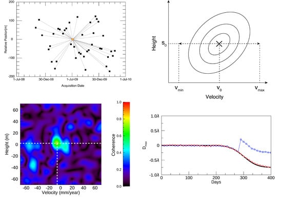
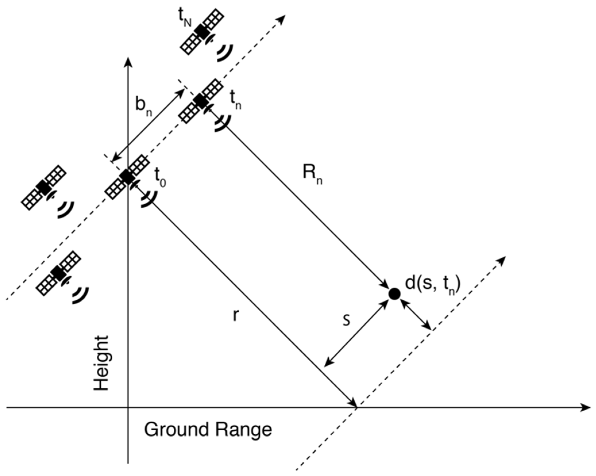
2.1. Multi-Baseline Model
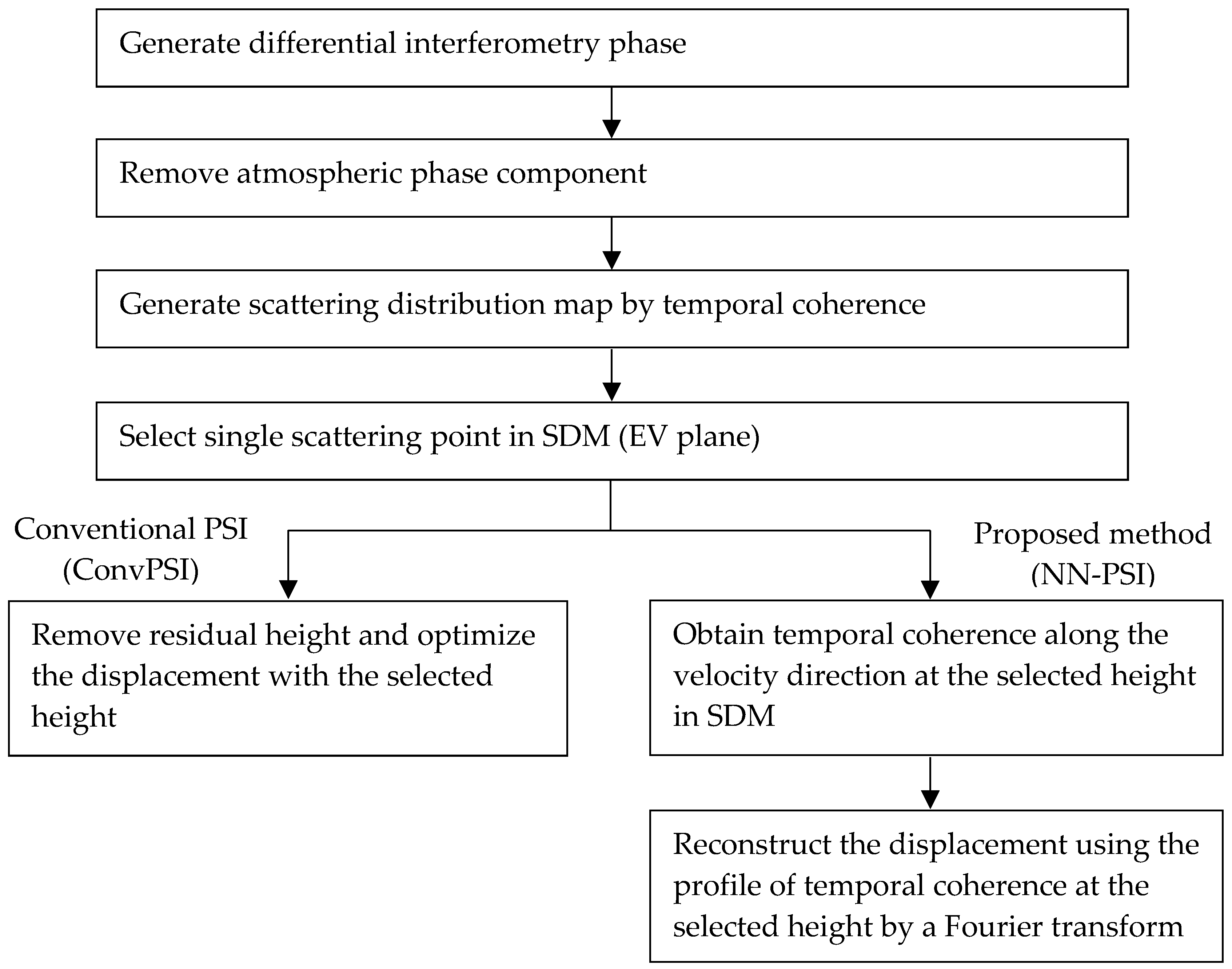
2.2. Calculation Procedure
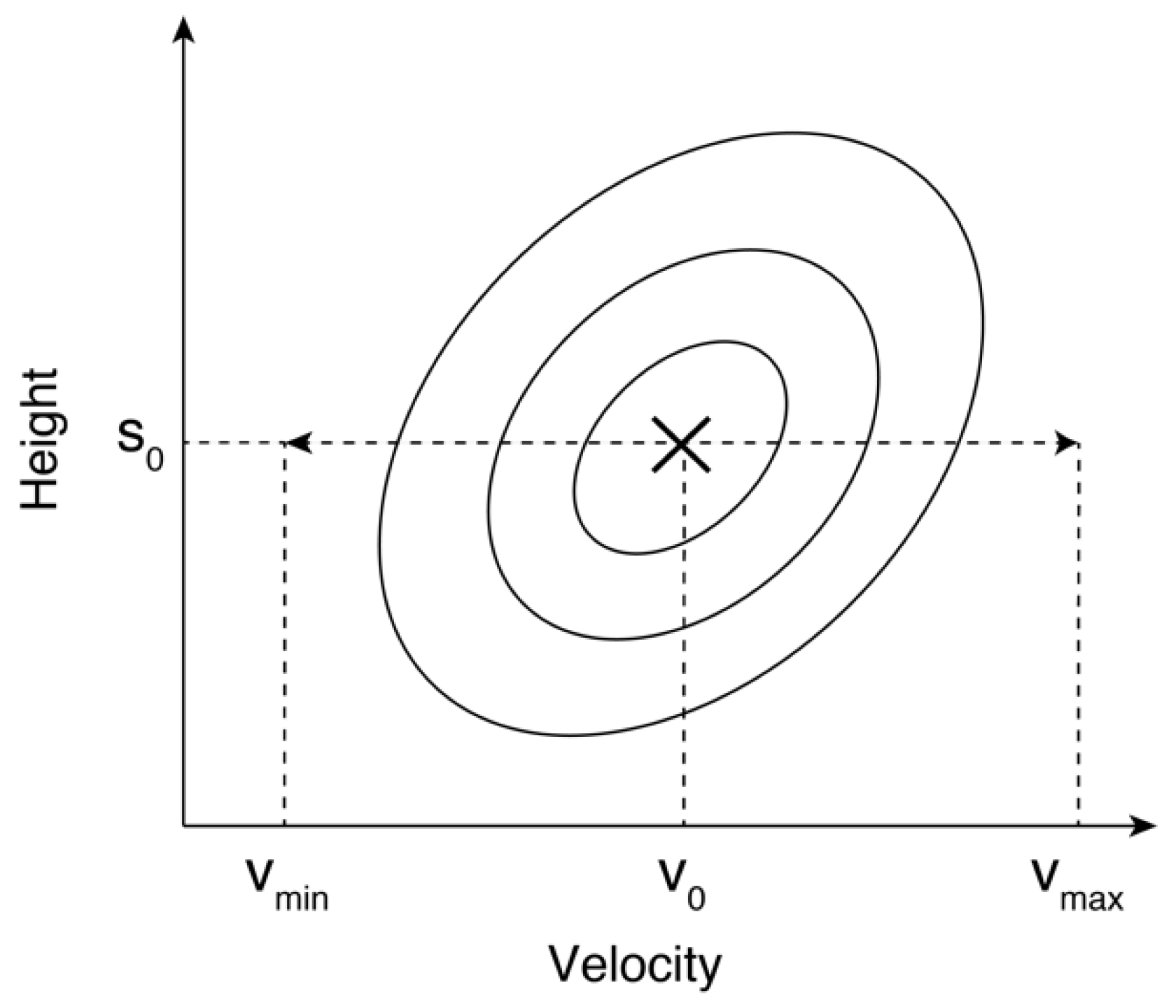
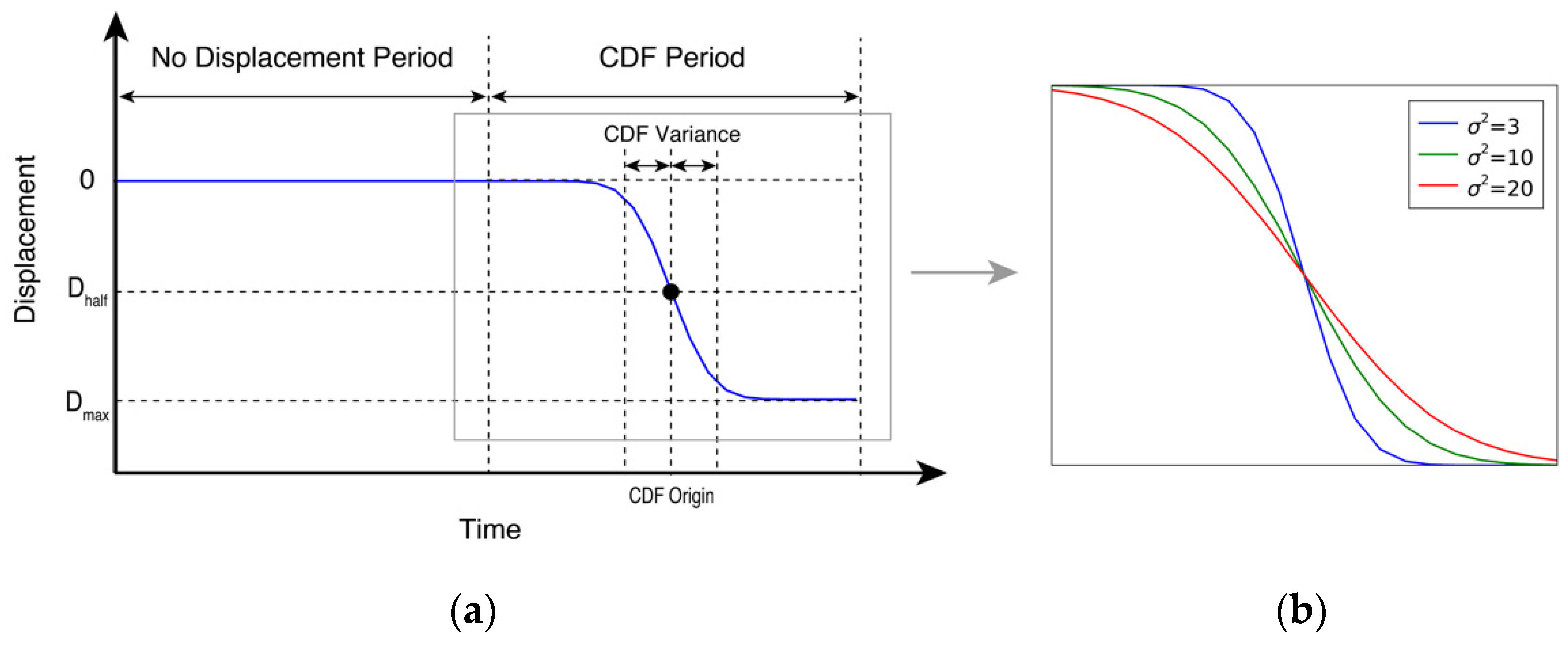
2.3. Scattering Distribution
2.4. ConvPSI
2.5. NN-PSI
3. Simulation
- The applicable displacements of NN-PSI were investigated by changing the magnitude and period of the displacements (simulation-1);
- How the velocity ranges that are used in the generation of SDM affect the resulting displacement with NN-PSI was investigated (simulation-2).
4. Simulation Results and Discussions
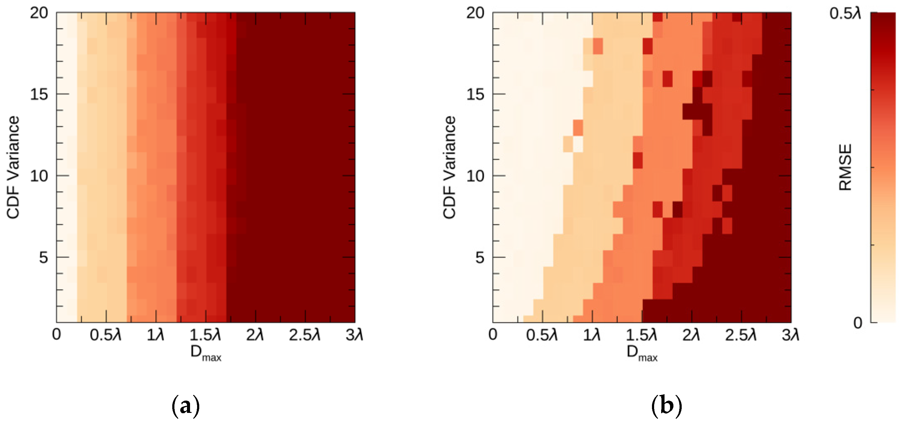
4.1. Simulation-1
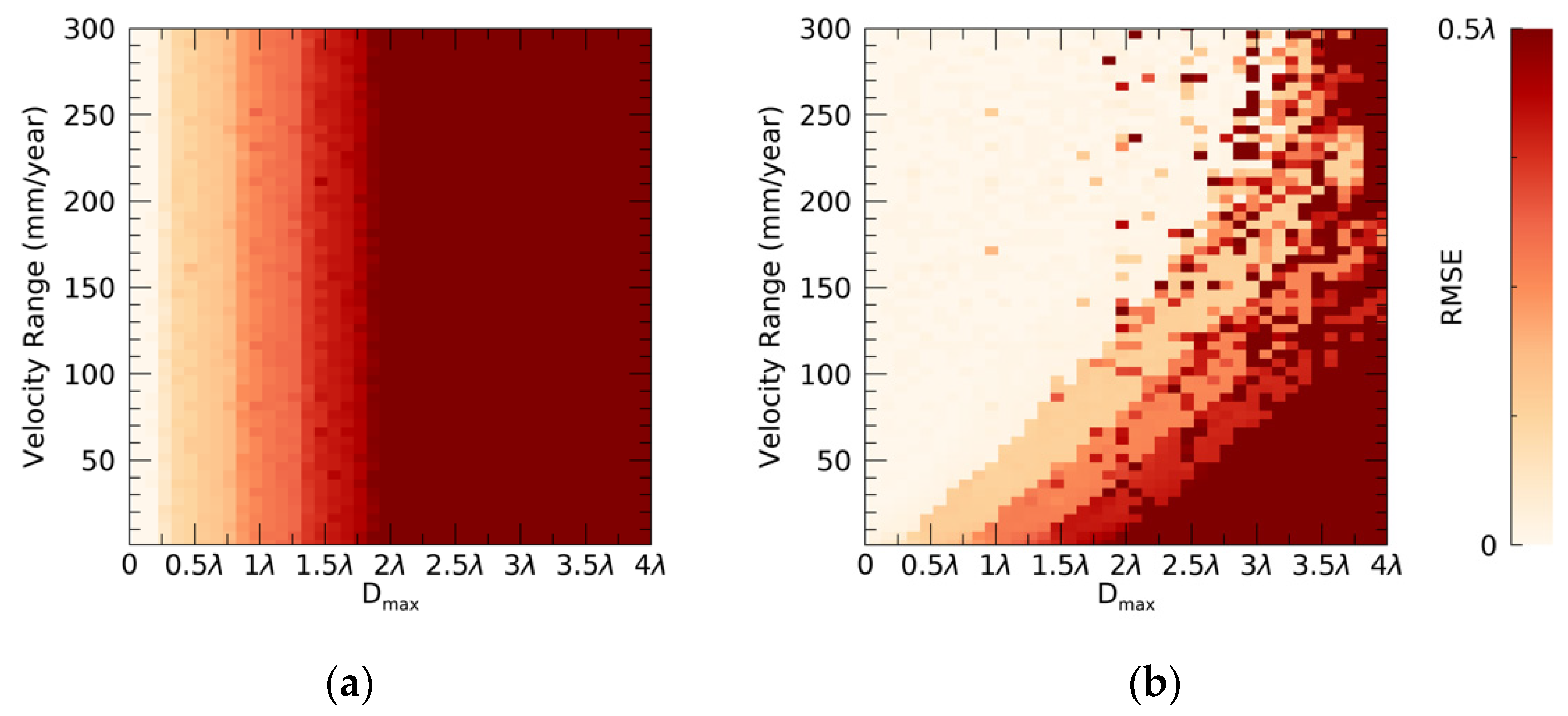
4.2. Simulation-2
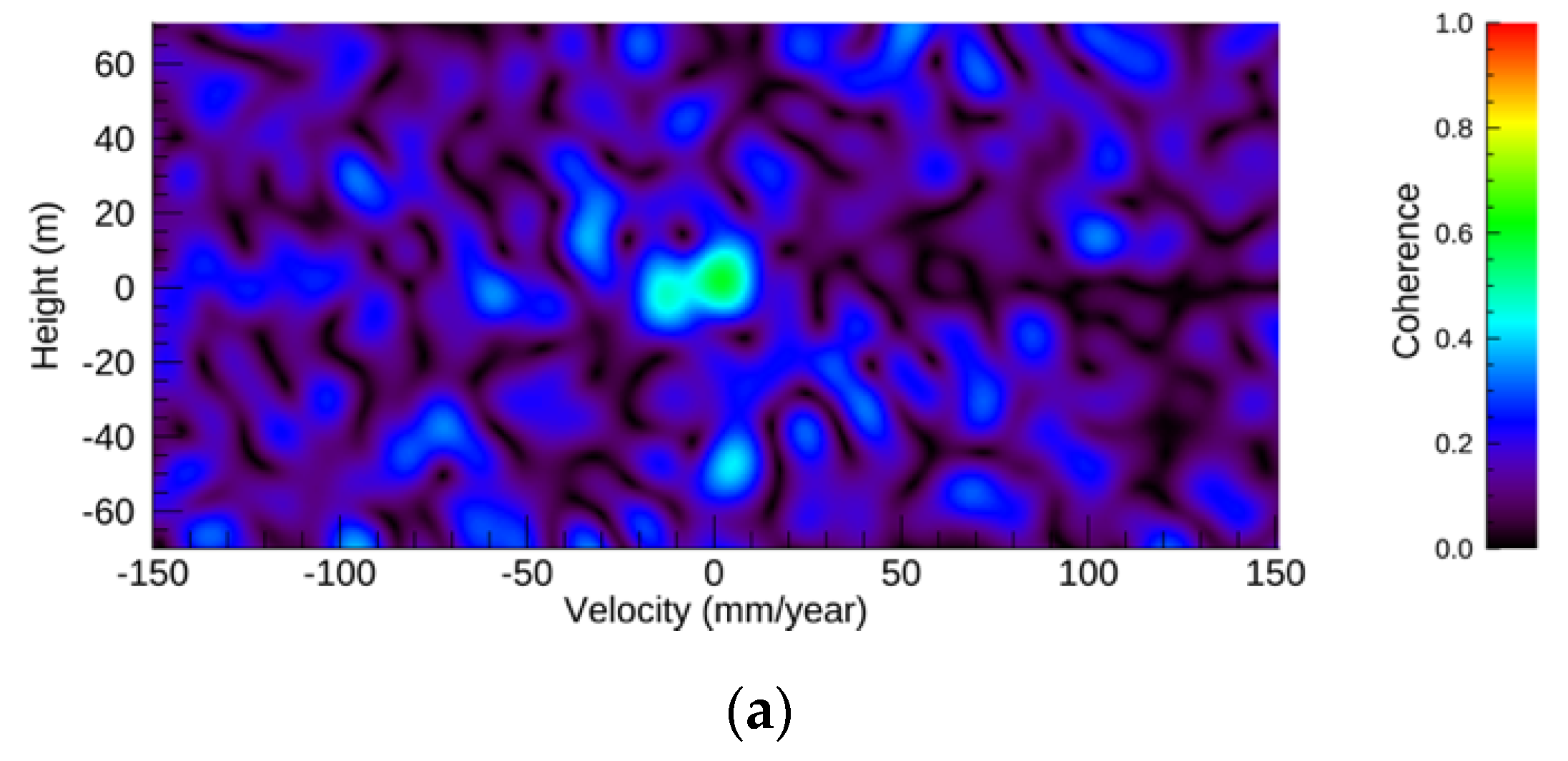
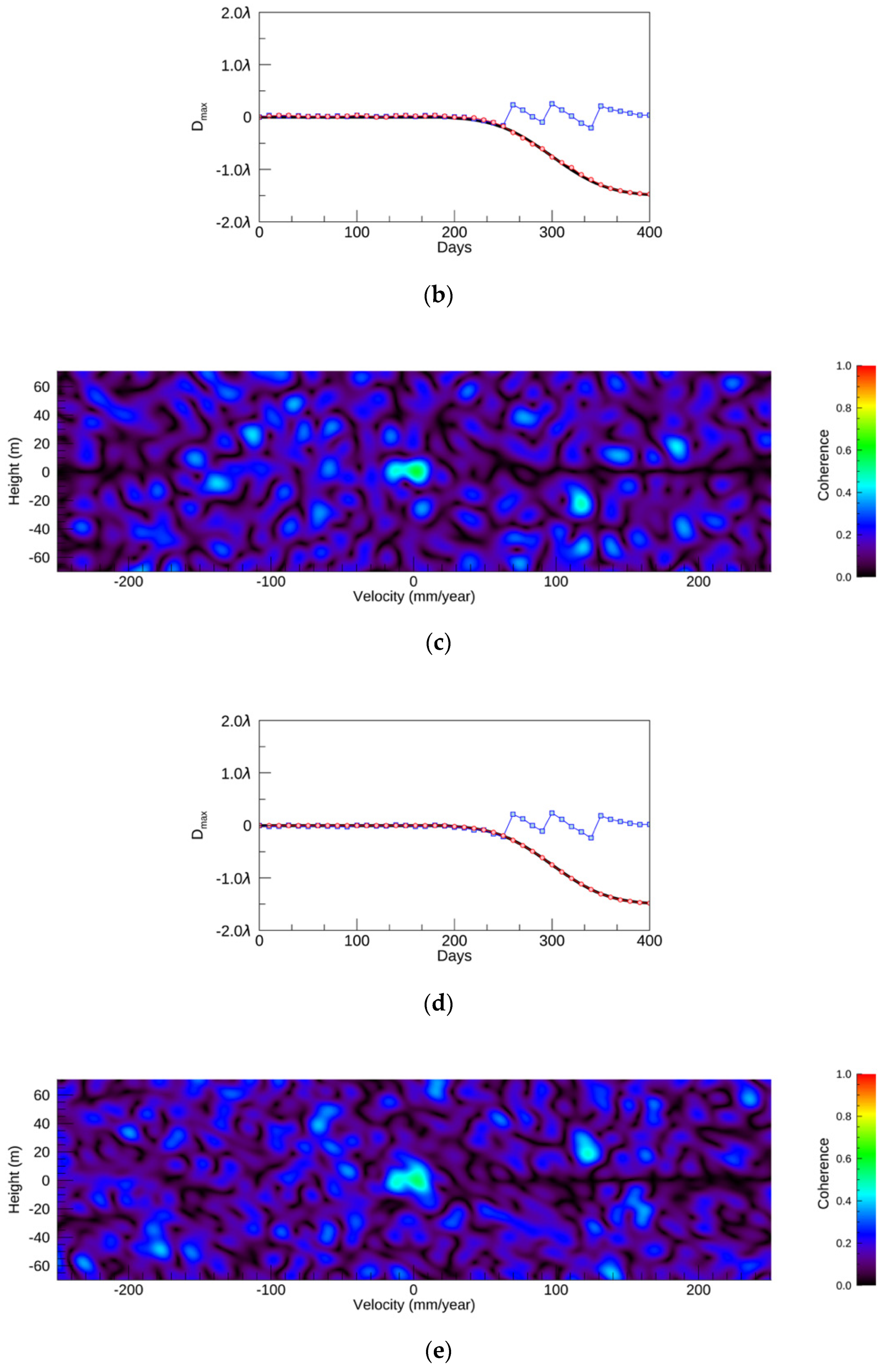
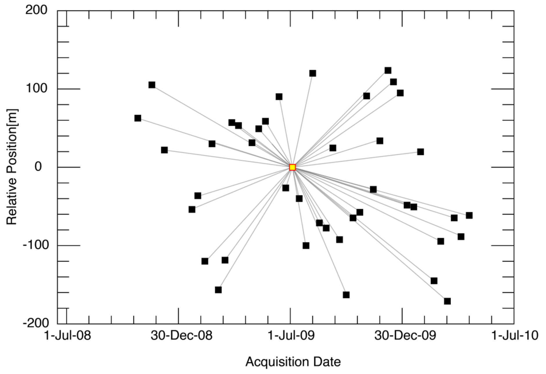
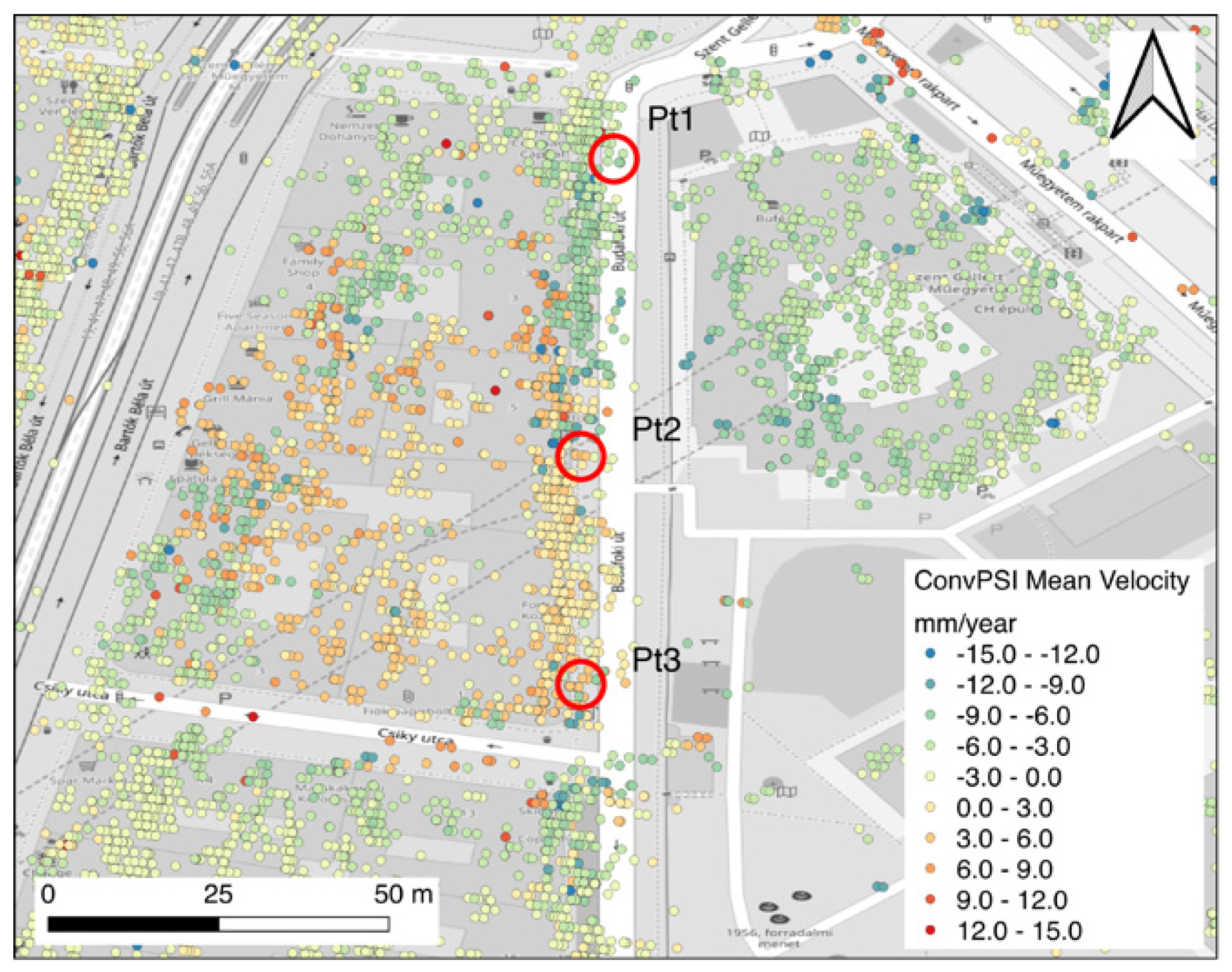
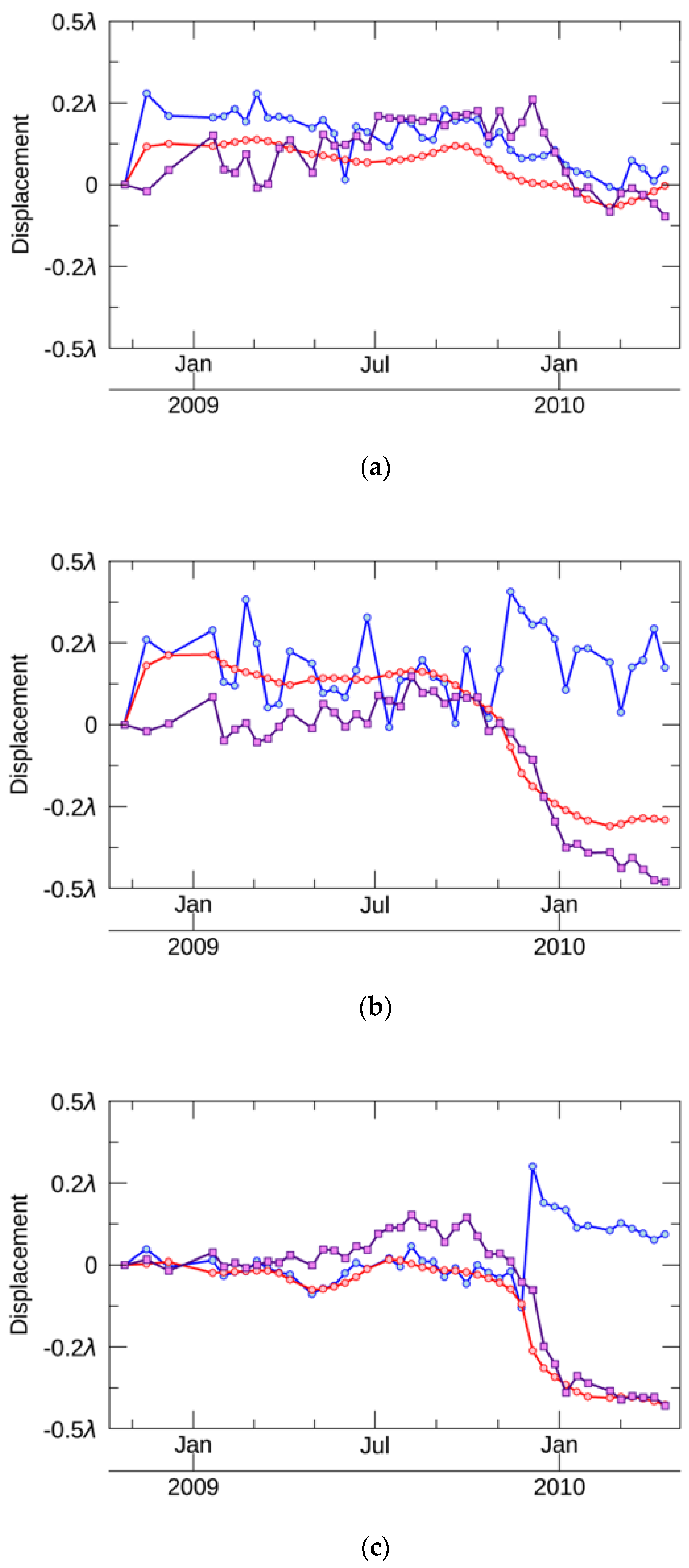
5. Experiment with Actual Observation Data
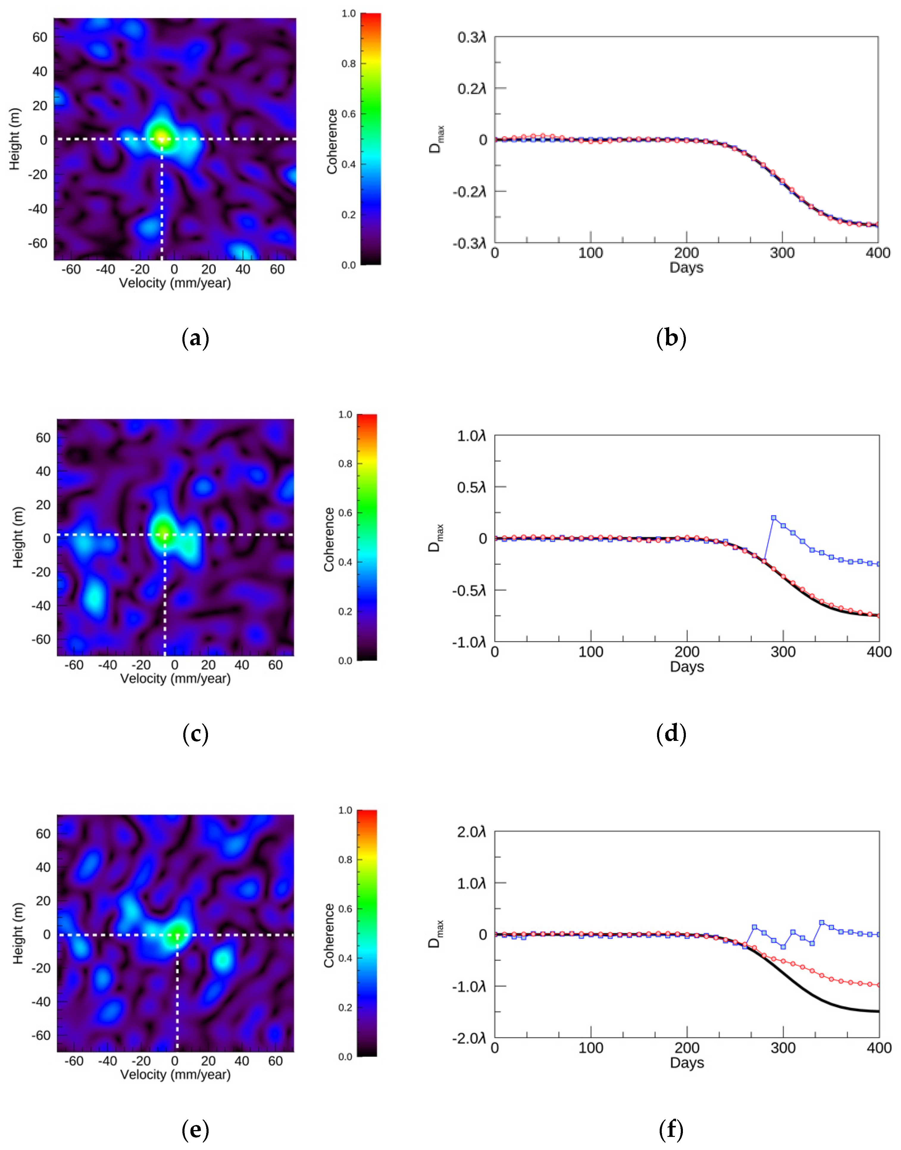
5.1. ConvPSI and NN-PSI
5.2. Comparison with SBAS Results
6. Conclusions
Author Contributions
Funding
Acknowledgments
Conflicts of Interest
References
- Rosen, P.A.; Hensley, S.; Joughin, I.R.I.; Li, F.K.; Madsen, S.N.; Rodriguez, E.; Goldstein, R.M. Synthetic aperture radar interferometry. Proc. IEEE 2000, 88, 333–382. [Google Scholar] [CrossRef]
- Gabriel, A.K.; Goldstein, R.M.; Zebker, H.A. Mapping small elevation changes over large areas—Differential radar interferometry. J. Geophys. Res. 1989, 94, 9183–9191. [Google Scholar] [CrossRef]
- Massonnet, D.; Rossi, M.; Carmona, C.; Adragna, F.; Peltzer, G.; Feigl, K.; Rabaute, T. The displacement field of the Landers earthquake mapped by radar interferometry. Nature 1993, 364, 138–142. [Google Scholar] [CrossRef]
- Peltzer, G.; Rosen, P. Surface Displacement of the 17 May 1993 Eureka Valley, California, Earthquake Observed by SAR Interferometry. Science 1995, 268, 1333–1336. [Google Scholar] [CrossRef] [PubMed]
- Hooper, A.J. A multi-temporal InSAR method incorporating both persistent scatterer and small baseline approaches. Geophys. Res. Lett. 2008, 35. [Google Scholar] [CrossRef]
- Pasquali, P.; Cantone, A.; Riccardi, P.; Defilippi, M.; Ogushi, F.; Gagliano, S.; Tamura, M. Mapping of Ground Deformations with Interferometric Stacking Techniques. Land Appl. Radar Remote Sens. 2014, 233–259. [Google Scholar] [CrossRef]
- Ferretti, A.; Prati, C.; Rocca, F. Permanent Scatterers in SAR Interferometry. IEEE Trans. Geosci. Remote Sens. 2001, 39, 8–20. [Google Scholar] [CrossRef]
- Farina, P.; Colombo, D.; Fumagalli, A.; Marks, F.; Moretti, S. Permanent Scatterers for landslide investigations: Outcomes from the ESA-SLAM project. Eng. Geol. 2006, 88, 200–217. [Google Scholar] [CrossRef]
- Colesanti, C.; Wasowski, J. Investigating landslides with space-borne Synthetic Aperture Radar (SAR) interferometry. Eng. Geol. 2006, 88, 173–199. [Google Scholar] [CrossRef]
- Tofani, V.; Raspini, F.; Catani, F.; Casagli, N. Persistent scatterer interferometry (PSI) technique for landslide characterization and monitoring. Remote Sens. 2013, 5, 1045–1065. [Google Scholar] [CrossRef]
- Zhao, F.; Mallorqui, J.J. Landslide Monitoring Using Multi-Temporal SAR Interferometry with Advanced Persistent Scatterers Identification Methods and Super High-Spatial Resolution TerraSAR-X Images. Remote Sens. 2018, 10, 921. [Google Scholar] [CrossRef]
- Sousa, J.J.; Bastos, L. Multi-temporal SAR interferometry reveals acceleration of bridge sinking before collapse. Nat. Hazards Earth Syst. Sci. 2013, 13, 659–667. [Google Scholar] [CrossRef]
- Lazecky, M.; Perissin, D.; Lei, L.; Qin, Y.; Scaioni, M. Plover Cove dam monitoring with spaceborne InSAR technique in Hong Kong. In Proceedings of the 2nd Joint International Symposium on Deformation Monitoring, Nottingham, UK, 9–11 September 2013. [Google Scholar]
- Fornaro, G.; Reale, D.; Verde, S. Bridge Thermal Dilation Monitoring with Millimeter Sensitivity via Multidimensional SAR Imaging. IEEE Geosci. Remote Sens. Lett. 2013, 10, 677–681. [Google Scholar] [CrossRef]
- Pratesi, F.; Tapete, D.; Terenzi, G.; Del, C.; Moretti, S. Rating health and stability of engineering structures via classification indexes of InSAR Persistent Scatterers. Int. J. Appl. Earth Obs. Geoinf. 2015, 40, 81–90. [Google Scholar] [CrossRef]
- Ishitsuka, K.; Tsuji, T.; Matsuoka, T.; Nishijima, J. Heterogeneous surface displacement pattern at the Hatchobaru geothermal field inferred from SAR interferometry time-series. Int. J. Appl. Earth Obs. Geoinf. 2016, 44, 95–103. [Google Scholar] [CrossRef]
- Wegmüller, U.; Walter, D.; Spreckels, V.; Werner, C.L.; Member, S. Nonuniform Ground Motion Monitoring with TerraSAR-X Persistent Scatterer Interferometry. IEEE Trans. Geosci. Remote Sens. 2010, 48, 895–904. [Google Scholar] [CrossRef]
- Raucoules, D.; Bourgine, B.; de Michele, M.; Le Cozannet, G.; Closset, L.; Bremmer, C.; Engdahl, M. Validation and intercomparison of Persistent Scatterers Interferometry: PSIC4 project results. J. Appl. Geophys. 2009, 68, 335–347. [Google Scholar] [CrossRef]
- Wasowski, J.; Bovenga, F. Investigating landslides and unstable slopes with satellite Multi Temporal Interferometry: Current issues and future perspectives. Engineering Geology 2014, 174, 103–138. [Google Scholar] [CrossRef]
- Crosetto, M.; Monserrat, O.; Cuevas-González, M.; Devanthéry, N.; Crippa, B. Persistent Scatterer Interferometry: A review. Isprs. J. Photogramm. Remote Sens. 2016, 115, 78–89. [Google Scholar] [CrossRef]
- Ferretti, A.; Prati, C.; Rocca, F. Nonlinear Subsidence Rate Estimation Using Permanent Scatterers in Differential SAR Interferometry. IEEE Trans. Geosci. Remote Sens. 2000, 38, 2202–2212. [Google Scholar] [CrossRef]
- Colesanti, C.; Ferretti, A.; Novali, F.; Prati, C.; Rocca, F. SAR Monitoring of Progressive and Seasonal Ground Deformation Using the Permanent Scatterers Technique. IEEE Trans. Geosci. Remote Sens. 2003, 41, 1685–1701. [Google Scholar] [CrossRef]
- Zhang, L.; Ding, X.; Lu, Z. Modeling PSInSAR Time Series Without Phase Unwrapping. IEEE Trans. Geosci. Remote Sens. 2011, 49, 547–556. [Google Scholar] [CrossRef]
- Ferretti, A.; Bianchi, M.; Prati, C.; Rocca, F. Higher-order permanent scatterers analysis. EURASIP J. Appl. Signal Process. 2005, 2005, 3231–3242. [Google Scholar] [CrossRef]
- Lombardini, F. Differential tomography: A new framework for SAR interferometry. IEEE Trans. Geosci. Remote Sens. 2005, 43, 37–44. [Google Scholar] [CrossRef]
- Fornaro, G.; Reale, D.; Serafino, F. Four-dimensional SAR imaging for height estimation and monitoring of single and double scatterers. IEEE Trans. Geosci. Remote Sens. 2009, 47, 224–237. [Google Scholar] [CrossRef]
- Zhu, X.X.; Bamler, R. Let’s Do the Time Warp: Multicomponent Nonlinear Motion Estimation in Differential SAR Tomography. IEEE Geosci. Remote Sens. Lett. 2011, 8, 735–739. [Google Scholar] [CrossRef]
- Budillon, A.; Crosetto, M.; Johnsy, A.C.; Monserrat, O.; Krishnakumar, V.; Schirinzi, G. Comparison of Persistent Scatterer Interferometry and SAR Tomography Using Sentinel-1 in Urban Environment. Remote Sens. 2018, 10, 1986. [Google Scholar] [CrossRef]
- Berardino, P.; Fornaro, G.; Lanari, R.; Sansosti, E. A new algorithm for monitoring localized deformation phenomena based on small baseline differential SAR interferograms. In Proceedings of the IEEE International Geoscience and Remote Sensing Symposium, Toronto, ON, Canada, 24–28 June 2002. [Google Scholar]
- Pepe, A.; Lanari, R. On the Extension of the Minimum Cost Flow Algorithm for Phase Unwrapping of Multitemporal Differential SAR Interferograms. IEEE Trans. Geosci. Remote Sens. 2006, 44, 2374–2383. [Google Scholar] [CrossRef]
- Gatelli, F.; Monti Guarnieri, A.; Parizzi, F.; Pasquali, P.; Prati, C.; Rocca, F. The wavenumber shift in SAR interferometry. IEEE Trans. Geosci. Remote Sens. 1994, 32, 855–865. [Google Scholar] [CrossRef]
- Pasquali, P.; Prati, C.; Rocca, F.; Seymour, M.; Fortuny, J.; Ohlmer, E.; Sieber, A.J. A 3-D SAR Experiment with EMSL Data. In Proceedings of the 1995 International Geoscience and Remote Sensing Symposium, IGARSS’95, Quantitative Remote Sensing for Science and Application, Firenze, Italy, 10–14 July 1995. [Google Scholar]
- Reigber, A.; Moreira, A. First Demonstration of Airborne SAR Tomography Using Multibaseline L-Band Data. IEEE Trans. Geosci. Remote Sens. 2000, 38, 2142–2152. [Google Scholar] [CrossRef]
- Lombardini, F.; Pauciullo, A.; Fornaro, G.; Reale, D.; Viviani, F. Tomographic Processing of Interferometric SAR Data. IEEE Signal Process. Mag. 2014, 50, 41–50. [Google Scholar]
- Fornaro, G.; Serafino, F.; Soldovieri, F. Three-dimensional focusing with multipass SAR data. IEEE Trans. Geosci. Remote Sens. 2003, 41(3), 507–517. [Google Scholar] [CrossRef]
- Maio, A.; De Fornaro, G.; Pauciullo, A. Detection of Single Scatterers in Multidimensional SAR Imaging. IEEE Trans. Geosci. Remote Sens. 2009, 47, 2284–2297. [Google Scholar] [CrossRef]
- Peter, K. Space Monitor for Hong Kong Settlement. Available online: https://tunneltalk.com/Satellite-imaging-Sep11-Satellite-eye-on-settlement.php (accessed on 17 September 2019).
- Corne, E. Satellite technology as an aid to map and monitor construction/infrastructure sites anywhere in the world. Proceedings of Geomatics Indaba, Ekurhuleni, South Africa, 11–13 August 2015. [Google Scholar]


| Items | Simulation-1 | Simulation-2 |
|---|---|---|
| Slant range distance | 700 km | |
| Incidence angle | 45° | |
| Baseline variance 1 | ±4% | |
| Backscatter coefficient | 5 dB | |
| Number of observations | 41 | |
| Observation interval | 10 days | |
| Total period | 410 days | |
| No-displacement period | 200 days | |
| CDF period | 210 days | |
| Search velocity range | ±70 mm/year | 0–±300 mm/year |
| CDF variance | 1–20 | 20 |
| Dmax (λ: wavelength) | 0–3λ | 0–4λ |
| Parameters | Values |
|---|---|
| Satellite sensor | TerraSAR-X |
| Monitoring period | 24 October 2008–16 April 2010 |
| Number of acquisitions | 42 |
| Time interval of the acquisitions | 11 days |
| Date of the master acquisition | 4 July 2009 |
| Incidence angle | 44.5° |
| Wavelength () | 31.066 mm |
| Method | Pt1 | Pt2 | Pt3 |
|---|---|---|---|
| ConvPSI | 0.31 | −0.14 | −0.66 |
| NN-PSI | 0.35 | 0.88 | 0.95 |
© 2019 by the authors. Licensee MDPI, Basel, Switzerland. This article is an open access article distributed under the terms and conditions of the Creative Commons Attribution (CC BY) license (http://creativecommons.org/licenses/by/4.0/).
Share and Cite
Ogushi, F.; Matsuoka, M.; Defilippi, M.; Pasquali, P. Improvement of Persistent Scatterer Interferometry to Detect Large Non-Linear Displacements with the 2π Ambiguity by a Non-Parametric Approach. Remote Sens. 2019, 11, 2467. https://doi.org/10.3390/rs11212467
Ogushi F, Matsuoka M, Defilippi M, Pasquali P. Improvement of Persistent Scatterer Interferometry to Detect Large Non-Linear Displacements with the 2π Ambiguity by a Non-Parametric Approach. Remote Sensing. 2019; 11(21):2467. https://doi.org/10.3390/rs11212467
Chicago/Turabian StyleOgushi, Fumitaka, Masashi Matsuoka, Marco Defilippi, and Paolo Pasquali. 2019. "Improvement of Persistent Scatterer Interferometry to Detect Large Non-Linear Displacements with the 2π Ambiguity by a Non-Parametric Approach" Remote Sensing 11, no. 21: 2467. https://doi.org/10.3390/rs11212467
APA StyleOgushi, F., Matsuoka, M., Defilippi, M., & Pasquali, P. (2019). Improvement of Persistent Scatterer Interferometry to Detect Large Non-Linear Displacements with the 2π Ambiguity by a Non-Parametric Approach. Remote Sensing, 11(21), 2467. https://doi.org/10.3390/rs11212467