Next Article in Journal
Greening Implication Inferred from Vegetation Dynamics Interacted with Climate Change and Human Activities over the Southeast Qinghai–Tibet Plateau
Previous Article in Journal
Crop Yield Estimation Using Time-Series MODIS Data and the Effects of Cropland Masks in Ontario, Canada
 
 
Comment published on 31 May 2020, see Remote Sens. 2020, 12(11), 1769.
Reply published on 31 May 2020, see Remote Sens. 2020, 12(11), 1771.
Technical Note

Local Climate Zone (LCZ) Map Accuracy Assessments Should Account for Land Cover Physical Characteristics that Affect the Local Thermal Environment

by
Brian Alan Johnson
1,* and
Shahab Eddin Jozdani
2
1
Natural Resources and Ecosystem Services, Institute for Global Environmental Strategies, 2108-11, Kamiyamaguchi, Hayama, Kanagawa 240-0115, Japan
2
Department of Geography and Planning, Queen’s University, Kingston, Ontario K7L 3N6, Canada
*
Author to whom correspondence should be addressed.
Remote Sens. 2019, 11(20), 2420; https://doi.org/10.3390/rs11202420
Submission received: 2 July 2019 / Revised: 3 September 2019 / Accepted: 16 October 2019 / Published: 18 October 2019
(This article belongs to the Section Urban Remote Sensing)

Abstract

:
Local climate zone (LCZ) maps are increasingly being used to help understand and model the urban microclimate, but traditional land use/land cover map (LULC) accuracy assessment approaches do not convey the accuracy at which LCZ maps depict the local thermal environment. 17 types of LCZs exist, each having unique physical characteristics that affect the local microclimate. Many studies have focused on generating LCZ maps using remote sensing data, but nearly all have used traditional LULC map accuracy metrics, which penalize all map classification errors equally, to evaluate the accuracy of these maps. Here, we proposed a new accuracy assessment approach that better explains the accuracy of the physical properties (i.e., surface structure, land cover, and anthropogenic heat emissions) depicted in an LCZ map, which allows for a better understanding of the accuracy at which the map portrays the local thermal environment.

Graphical Abstract

1. Introduction

Mapping and analysis of local climate zones (LCZs), i.e., landscape units with distinct screen-height temperature regimes [1], has become a popular research topic in the fields of remote sensing and urban climatology in recent years. The LCZ classification scheme divides the landscape into 17 classes, each having different surface structure, land cover, and anthropogenic heat emission characteristics (hereafter “physical characteristics”) that affect the local air temperature [2]. LCZ maps have become an important source of data for studies on urban climatology [2,3,4,5] and urban planning [6]. In a more general context, the LCZ classification scheme has also been suggested as a standardized framework for the mapping of urban form at the global scale, as it can provide information on the basic physical properties of any urban area [7].
LCZ maps are typically generated by analyzing satellite images using semi-automated image classification algorithms. The most common approach involves performing supervised classification of Landsat satellite imagery using the random forest classification algorithm [8], and this approach has been termed the “world urban database and access portals tools” (WUDAPT) protocol [7]. The WUDAPT protocol has been applied successfully in many LCZ mapping studies in different geographic regions [4,5,6,9,10]. To build on the WUDAPT approach, some studies have proposed the use of additional remote sensing datasets, e.g., nighttime optical imagery [11], nighttime thermal infrared imagery [12], synthetic aperture radar data [9], or LiDAR data [13]. Other studies have proposed incorporating ancillary GIS datasets in the image classification workflow, e.g., OpenStreetMap data [11,14], and/or the use of alternative classification algorithms (e.g., convolutional neural networks [11]).
No matter the input data or image classification method used, all LCZ maps contain some degree of classification errors. As with all land use/land cover (LULC) map products, it is important to quantify these errors, e.g., in terms of producer’s accuracy (errors of omission), user’s accuracy (errors of commission), and overall accuracy [15]. Traditional LULC map accuracy assessment metrics are calculated by comparing the estimated (i.e., mapped) LULC type with the reference (i.e., “ground truth”) LULC at sample pixel locations, and making a binary decision as to whether each sample location is correctly/incorrectly classified [16]. This purely thematic approach which penalizes all mapping errors equally, however, does not allow a user to adequately interpret the map’s accuracy for modeling specific physical processes (e.g., rainfall runoff [17] or urban microclimate). In the case of LCZ mapping, some LCZ types are quite similar to one another in terms of their physical characteristics (e.g., “LCZ 2: compact mid-rise” and “LCZ 3: compact low-rise”), and a misclassification between two physically similar LCZ types will not pose as great a problem for urban climate studies as a misclassification between two physically dissimilar LCZ types (e.g., “LCZ 1: compact high-rise” and “LCZ A: dense trees”). Evidence of this can be seen in Bechtel et al. [3], where, based on an analysis of LCZ maps and land surface temperature data from 50 cities around the world, LCZ types with more similar physical characteristics were found to have more similar surface urban heat island intensities. Similar findings were also reported in individual case studies [2,10,12].
Based on the above, it is clear that LCZ map accuracy assessments should be conducted in a way that takes into account the physical characteristics of each LCZ type, e.g., by applying a greater penalization to classification errors between more dissimilar LCZ types. To our knowledge, however, only one prior study has attempted to incorporate such an approach. Bechtel et al. [18] proposed to weight the traditional LULC map error matrix using a multiplier that accounts for the similarity between LCZ types (based on the properties of openness, height, surface cover, and thermal inertia). Their idea of weighting the error matrix has merit, but their proposed methodology had two main shortcomings: (1) the determined weights were subjective and not fully transparent (e.g., no equations provided to explain how they were derived); and (2) the weights incorrectly applied a higher penalty to the misclassification of more physically similar LCZ types. The first shortcoming limits the flexibility and transferability of their methodology, as it is not possible to develop locally-optimized weights for a specific study site (i.e., weights based on the typical physical properties of the LCZs in that specific study site) if no equations are provided. The second shortcoming results in the assignment of lower penalizations to map classification errors that have larger impacts on the predicted microclimate (i.e., to misclassifications of physically dissimilar LCZ types), which is the opposite of what is logical. In the literature related to LCZ mapping, most past studies have used the traditional LULC map error matrix to evaluate LCZ mapping accuracy [4,7,12,14], while a few studies have used the method proposed by Bechtel et al. [3,18]. Thus, it is critical to develop more suitable LCZ map accuracy assessment metrics.

Proposed Approach

The objective of this study is to provide an objective and generic method for LCZ map accuracy assessment, taking into account the typical physical characteristics of each LCZ type that affect the local thermal environment. Our approach involves weighting the traditional LULC map error matrix using a “LCZ dissimilarity metric”, calculated based on the degree of dissimilarity between the classification result (i.e., mapped LCZ type) and the reference data in terms of the estimated surface geometry, surface cover, and thermal inertia characteristics. The values of this LCZ dissimilarity metric can range from 0 (no penalty for misclassification) to 1 (full penalty for misclassification, which is equivalent to value of the traditional error matrix). The weighted producer’s/user’s/overall accuracy measures that can be derived from our weighted error matrix indicate the level of similarity between the estimated and reference (“ground truth”) landscape physical characteristics depicted in the map, which allows for a better understanding of the map’s accuracy in portraying the local thermal environment. Our proposed methodology is intended to be generic enough to apply in any study site, although site-specific information on the reference physical characteristics of each LCZ type could alternatively be used (in place of the values in Figure 1), if available.

2. Materials and Methods

2.1. Generating the LCZ Dissimilarity Metric

The proposed LCZ dissimilarity metric takes into account nine of the ten physical parameters presented in Stewart and Oke [1] as the basis for LCZ identification:
  • sky view factor (SV), i.e., fraction of sky hemisphere visible from ground level;
  • aspect ratio (AR), i.e., average height-to-width ratio of street canyons/building spacing/tree spacing;
  • mean building/tree height (H);
  • terrain roughness class (TR), based on Davenport et al.’s [19] terrain roughness classification scheme;
  • building surface fraction (BF);
  • impervious surface fraction (IF);
  • surface admittance (SA), i.e., capacity of surface to accept or release heat;
  • surface albedo (A); and
  • anthropogenic heat flux (AH).
The remaining parameter given in Stewart and Oke [1], pervious surface fraction, was not included for our calculations because it is inversely correlated with the impervious surface fraction parameter.
To calculate the LCZ dissimilarity metric, we first determined the average value of each parameter, for each LCZ type, based on the value ranges provided in Stewart and Oke [1] (see Figure 1 for all of these average values). To account for the different minimum–maximum ranges of the nine parameters, we normalized all of the derived average values to a 0–1 range using the following equation:
Pnorm = (PPmin)/(PmaxPmin),
where P is the average value of a parameter, Pmax and Pmin are the maximum and minimum P values of the parameter (among all LCZ types), and Pnorm is the normalized P value. Table A1 shows the Pnorm values calculated for each LCZ type.
As the second step, we calculated the average (absolute value) difference between the Pnorm values of each pairwise combination of LCZ types (Dij). Dij is given by:
Dij = (ǀSViSVjǀ + ǀARiARjǀ + ǀHiHjǀ + ǀTRiTRjǀ + ǀBFiBFjǀ +
ǀIFiIFjǀ + ǀSAiSAjǀ + ǀAiAjǀ + ǀAHiAHjǀ)/9,
where i and j indicate two LCZ types i and j; and SV, AR, H, TR, BF, IF, SA, A, and AH are the Pnorm values of the parameters sky view factor, aspect ratio, mean building/tree height, terrain roughness, building surface fraction, impervious surface fraction, surface admittance, surface albedo, and anthropogenic heat flux, respectively. For “LCZ A: Dense trees” the surface admittance parameter is unknown [1], so this parameter was excluded from Dij calculations involving “LCZ A” (and the numerator of Equation (2) was divided by 8 instead of 9). All of the resultant Dij values are reported in Table 1, with higher values indicating a greater dissimilarity between two LCZ classes in terms of their surface structure, land cover, and anthropogenic heat flux properties. These Dij values represent our proposed LCZ dissimilarity metric. From Table 1, it can be seen that the two most similar LCZ types are “LCZ 5: Open mid-rise” and “LCZ 6: Open low-rise” (Dij = 0.08), while the two most dissimilar LCZ types are “LCZ 1: Compact high-rise” and “LCZ G: Water” (Dij = 0.80).

2.2. Using the LCZ Dissimilarity Metric to Weight the Traditional Error Matrix

A traditional LULC map error matrix is generated by systematically comparing the remote sensing-derived LULC map and the reference LULC dataset at sample pixel locations. The central part of the matrix is an array of number k × k in size, where k is equal to the number of LULC types in the map [15]. Rows in the error matrix represent the mapped LULC information at each sample location, columns represent the reference information, and the intersection of rows and columns summarize the number of samples mapped as a particular LULC type relative to the reference data [15]. From this error matrix, overall accuracy is calculated as the fraction of all samples that are correctly classified, while producer’s accuracy is calculated for each LULC type as the number of correctly classified samples divided by the total number of reference samples belonging to that LULC type (i.e., column total), and user’s accuracy is calculated for each LULC type as the number of correctly classified samples divided by the total number of samples mapped as that LULC type (i.e., row total).
A weighted error matrix, which accounts for the dissimilarity between each pair of LCZ types, can be derived by multiplying the values in the traditional error matrix by the corresponding LCZ dissimilarity metric (Dij) values presented in Table 2. The result of this weighting is that misclassifications between two physically similar LCZ classes receive a lower penalty in the calculation of producer’s accuracy/user’s accuracy/overall accuracy, as these classification errors will have less impact on the thermal properties that can be estimated from the LCZ map. On the other hand, misclassifications between two dissimilar LCZ types are applied with a higher penalty (up to 1, i.e., complete misclassification, in the case of highly dissimilar LCZ types). For correctly classified sample pixels, no penalty is applied because no misclassification exists, and the values are equivalent to those of the traditional error matrix.
This proposed approach to derive a weighed error matrix—and corresponding weighted producer’s accuracy/user’s accuracy/overall accuracy values—is quite similar to the approach used to calculate “weighted accuracy” in Bechtel et al. [18], but the previous study incorrectly applied greater penalties for misclassification between physically similar LCZ types rather than physically dissimilar LCZ types.

3. Results and Discussion

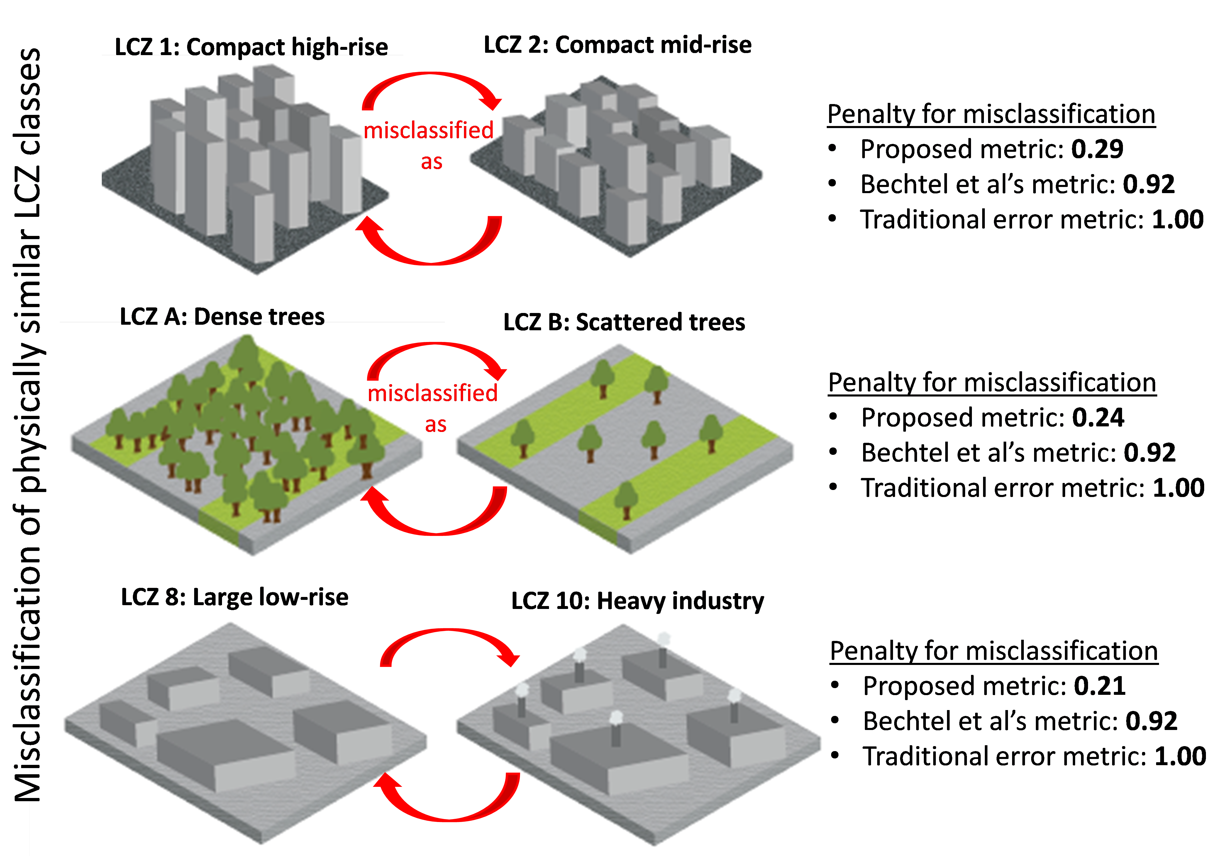
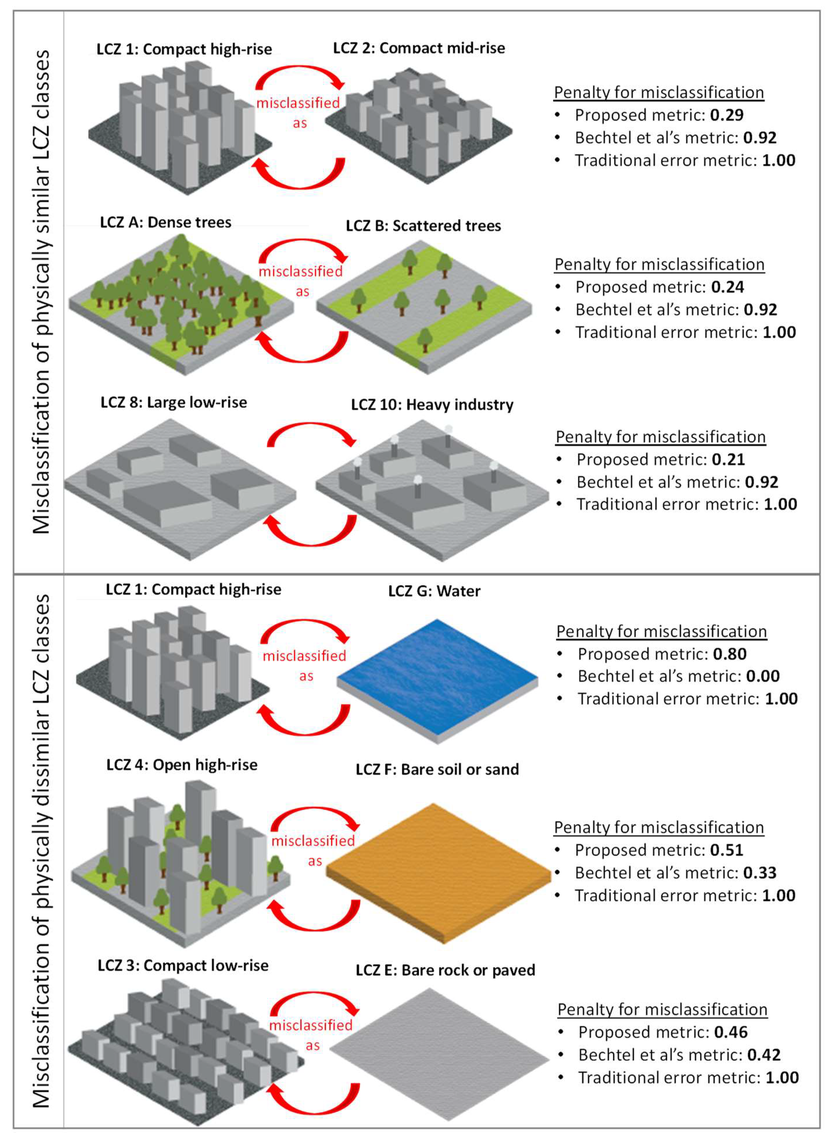
3.1. Comparison of Our LCZ Dissimilarity Metric with a Reference and the Traditional Error Metric

Figure 2 shows several examples of how the misclassification penalties derived by our LCZ dissimilarity metric differ from those of Bechtel et al. [18] and the traditional error matrix. As can be seen in the figure, compared to the metric of Bechtel et al. [18], our approach resulted in a lower penalty being applied to the misclassification of physically similar LCZ classes, and a higher penalty being applied to the misclassification of physically dissimilar LCZ classes. Thus, our weighted error matrix should give a better indication of how accurately a LCZ map depicts the local thermal environment.

3.2. Demonstration of Proposed Approach Using a Synthetic Dataset

In this section, we used a synthetic dataset to demonstrate the processes of generating a weighted error matrix, and calculating weighted overall/producer’s/user’s accuracy from the weighted error matrix. We elected to use a synthetic dataset here rather than real data to illustrate the metric calculations in a simpler way, i.e., without delving into explanations of the image data, training data, classification algorithm, etc., which would be needed if a real remote sensing dataset was used.
Table 2 shows a traditional (unweighted) error matrix for this synthetic dataset. The matrix contains 12 LCZ types, with 5 LCZ types assumed to not be present (missing LCZs is a common case, in practice). Table 3 shows the weighted error matrix, after the values in Table 2 have been multiplied by the LCZ dissimilarity metric values in Table 1. From the traditional error matrix, the overall accuracy (OA) of the LCZ map is calculated to be 0.76, while producer’s accuracy (PA) values range from 0.06–1.0 and user’s accuracy (UA) values range from 0.03–1.0. For the weighted error matrix, the weighted overall accuracy (wOA) value is calculated as 0.92, while the weighted producer’s accuracy (wPA) values range from 0.22–1.0 and the weighted user’s accuracy (wUA) values range from 0.14–1.0. Comparing the cell values of the two error matrices, it is evident that the differences between the PA/wPA values and UA/wUA values were greater for LCZ types that had been mostly misclassified as other physically similar LCZ types (e.g., misclassifications among the urban LCZ types; LCZ 1–10). This is because the misclassification penalties (i.e., Dij values) for these types of errors were relatively low under our proposed approach. From the comparison of the two matrices is also clear that the values in the weighted error matrix are always less than or equal to those of the traditional error matrix, and this is true because no pairwise combination of LCZs has a Dij value > 1.

3.3. Potential, Limitations, and Alternative Implementations of Proposed Approach

The weighted accuracy measures calculated using our proposed approach, wOA in particular, can serve as the basis for comparing multiple classified LCZ maps of the same study site—e.g., using different input datasets, different classification algorithms, and/or different classification variables—to identify the most accurate classified map. In this way, a LCZ map that best portrays the local thermal environment of a study site can be selected, allowing for more accurate simulations of urban microclimate to be conducted using other spatially-explicit models (e.g., the Weather Research Forecasting model [20]), and (ideally) for more climate-sensitive urban planning practices to be adopted.
One potential limitation of our approach, however, is that the values of the LCZ dissimilarity metric can only range from 0–1 (or more specifically, from 0.08–0.80 using our generic approach). The significance is that the weighted accuracy values cannot be lower than their unweighted counterparts, because the multiplier for misclassification is always assumed to be 1 in the traditional error matrix. Thus, our error matrix weighting approach is somewhat akin to the process of merging of LCZs into fewer, more general LULC categories (e.g., either “built-up” or “natural” [9,18]) for accuracy assessment, but our approach is more of a partial merging (unless Dij = 0).
A second limitation of our approach is that some of the weighted accuracy metrics may be more difficult to interpret than the traditional metrics. wOA can be generally understood as the degree of accuracy at which the generated LCZ map estimates the physical characteristics of the landscape relevant to the local thermal environment. The wPA and wUA values, however, are more difficult to interpret and should be used with caution. Additionally, the LCZ dissimilarity metric weighted accuracy metrics are based the typical physical characteristics (surface structure, land cover, and anthropogenic heat emissions) of each LCZ type, as identified in Stewart and Oke [1]. In reality, however, these physical characteristics can vary from region to region [11]. Our approach is intended to be generic enough to use anywhere, but the collection and usage of locally appropriate parameter values would be beneficial, when feasible.
Finally, we should point out that for some applications (e.g., LULC change assessment or urban planning), an LCZ map creator or map user may be concerned with both the map’s thematic accuracy and the accuracy of the physical characteristics depicted in the map. Considering this, rather than simply use OA or wOA to evaluate an LCZ map’s accuracy, an alternative would be to combine these two metrics, e.g., based on the mean average accuracy of the two metrics [(OA + wOA)/2] or the harmonic mean (F1-measure) [(2 × OA × wOA)/(OA + wOA)] [21]. In this way, multiple classified LCZ maps could be compared to identify one that achieves the desired trade-off between thematic and physical accuracy. Indeed, it is relatively common to interpret and/or combine multiple measures of accuracy in remote sensing studies, e.g., for image classification [18,22,23], image segmentation [24,25,26], or image enhancement [27]. In the case of our synthetic dataset, the mean average accuracy of the two metrics would be equal to 0.840, while the F1-measure would be equal to 0.837.

4. Conclusions

In this study, we presented a new approach for evaluating the accuracy of local climate zone (LCZ) maps. The proposed approach takes into account the dissimilarity between different LCZ types in terms of nine physical characteristics (sky view factor, aspect ratio, mean building/tree height, terrain roughness, building surface fraction, impervious surface fraction, surface admittance, surface albedo, and anthropogenic heat flux), and allows for a better understanding of the accuracy at which LCZ maps depict the local thermal environment of the landscape. We have presented a generic approach based on the typical physical parameters of each LCZ type (as identified in [1]), but it is also possible to optimize the approach for a specific location, considering the locally-appropriate physical characteristics of each LCZ type, by substituting locally-specific values for the values given in Figure 1. In contrast, the previous approach developed by Bechtel et al. does allow for this kind of optimization, as equations for calculating the error matrix weights are not provided. Although our proposed approach has some limitations, it is more suitable for evaluating the accuracy of LCZ maps than the traditional land use/land cover accuracy assessment approach that considers only map thematic accuracy, and is also more suitable than the existing physically-based LCZ map accuracy assessment approach (i.e., that proposed by Bechtel et al.).
Finally, although in this study we focused only on LCZ map accuracy assessment, there is a need to develop other application-specific LULC map accuracy assessment approaches, as LULC maps are now being used as input data to model various physical processes. Our proposed approach could be slightly modified for use in other application domains. For example, to better evaluate the accuracy of LULC maps used as inputs for hydrological models, it would be necessary to account for the dissimilarity between LULC classes in terms of their hydrological properties (e.g., typical rainfall runoff and/or groundwater infiltration rates of different LULC types) rather than their thermal properties.

Author Contributions

Conceptualization, B.A.J.; methodology, B.A.J. and S.E.J; validation, B.A.J, and S.E.J.; formal analysis, B.A.J.; investigation, B.A.J.; resources, B.A.J.; data curation, B.A.J. and S.E.J.; writing—original draft preparation, B.A.J.; writing—review and editing, S.E.J.; visualization, B.A.J.

Funding

This research was supported by the Environment Research and Technology Development Fund (S-15-1(4) Predicting and Assessing Natural Capital and Ecosystem Services (PANCES)) of the Ministry of the Environment, Japan.

Conflicts of Interest

The authors declare no conflict of interest.

Appendix A

Table A1. Pnorm values for each LCZ type. Note: SV, AR, H, TR, BF, IF, SA, A, and AH columns show the Pnorm values of the parameters sky view factor, aspect ratio, mean building/tree height, terrain roughness, building surface fraction, impervious surface fraction, surface admittance, surface albedo, and anthropogenic heat flux, respectively.
LCZ Type SVARHTRBFIFSAA AH
1 0.1331.0001.0001.0000.6430.5000.7890.0001.000
2 0.3330.5410.4670.7860.7140.3891.0000.0000.214
3 0.2670.4390.1730.7140.7140.3330.6320.0000.214
4 0.5330.5921.0000.9290.3570.3330.7370.0780.143
5 0.6000.1940.4670.6430.3570.3890.8420.0780.071
6 0.7330.1940.1730.6430.3570.3330.6320.0780.071
7 0.2000.5920.0800.5001.0000.0560.3680.2220.100
8 0.8670.0610.1730.5710.5000.5560.6320.1110.143
9 0.9330.0510.1730.6430.1430.0560.5260.0780.029
10 0.7330.1220.2000.6430.2860.2780.8950.0220.857
A 0.0000.7960.4401.0000.0000.000n/a0.0000.000
B 0.6000.1840.2400.6430.0000.0000.0000.1110.000
C 0.8670.2350.0270.5000.0000.0000.2110.1670.000
D 1.0000.0000.0130.3570.0000.0000.5260.1110.000
E 1.0000.0000.0030.0710.0001.0001.0000.1670.000
F 1.0000.0000.0030.0710.0000.0000.1050.2780.000
G 1.0000.0000.0000.0000.0000.0000.6321.0000.000

References

  1. Stewart, I.D.; Oke, T.R. Local climate zones for urban temperature studies. Bull. Am. Meteorol. Soc. 2012, 93, 1879–1900. [Google Scholar] [CrossRef]
  2. Stewart, I.D.; Oke, T.R.; Krayenhoff, E.S. Evaluation of the “local climate zone” scheme using temperature observations and model simulations. Int. J. Climatol. 2014, 34, 1062–1080. [Google Scholar] [CrossRef]
  3. Bechtel, B.; Demuzere, M.; Mills, G.; Zhan, W.; Sismanidis, P.; Small, C.; Voogt, J. SUHI analysis using Local Climate Zones—A comparison of 50 cities. Urban Clim. 2019, 28, 100451. [Google Scholar] [CrossRef]
  4. Wang, R.; Cai, M.; Ren, C.; Bechtel, B.; Xu, Y.; Ng, E. Detecting multi-temporal land cover change and land surface temperature in Pearl River Delta by adopting local climate zone. Urban Clim. 2019, 28, 100455. [Google Scholar] [CrossRef]
  5. Wang, R.; Ren, C.; Xu, Y.; Lau, K.K.L.; Shi, Y. Mapping the local climate zones of urban areas by GIS-based and WUDAPT methods: A case study of Hong Kong. Urban Clim. 2018, 24, 567–576. [Google Scholar] [CrossRef]
  6. Perera, N.G.R.; Emmanuel, R. A “Local Climate Zone” based approach to urban planning in Colombo, Sri Lanka. Urban Clim. 2018, 23, 188–203. [Google Scholar] [CrossRef]
  7. Bechtel, B.; Alexander, P.; Böhner, J.; Ching, J.; Conrad, O.; Feddema, J.; Mills, G.; See, L.; Stewart, I. Mapping Local Climate Zones for a Worldwide Database of the Form and Function of Cities. ISPRS Int. J. Geo Inf. 2015, 4, 199–219. [Google Scholar] [CrossRef] [Green Version]
  8. Breiman, L. Random Forests. Mach. Learn. 2001, 45, 5–32. [Google Scholar] [CrossRef] [Green Version]
  9. Demuzere, M.; Bechtel, B.; Middel, A.; Mills, G. Mapping Europe into local climate zones. PLoS ONE 2019, 14, e0214474. [Google Scholar] [CrossRef]
  10. Shi, Y.; Lau, K.K.L.; Ren, C.; Ng, E. Evaluating the local climate zone classification in high-density heterogeneous urban environment using mobile measurement. Urban Clim. 2018, 25, 167–186. [Google Scholar] [CrossRef]
  11. Qiu, C.; Schmitt, M.; Mou, L.; Ghamisi, P.; Zhu, X.X. Feature importance analysis for local climate zone classification using a residual convolutional neural network with multi-source datasets. Remote Sens. 2018, 10, 1572. [Google Scholar] [CrossRef]
  12. Cai, M.; Ren, C.; Xu, Y.; Lau, K.K.L.; Wang, R. Investigating the relationship between local climate zone and land surface temperature using an improved WUDAPT methodology—A case study of Yangtze River Delta, China. Urban Clim. 2018, 24, 485–502. [Google Scholar] [CrossRef]
  13. Zhao, C.; Jensen, J.; Weng, Q.; Currit, N.; Weaver, R. Application of airborne remote sensing data on mapping local climate zones: Cases of three metropolitan areas of Texas, U.S. Comput. Environ. Urban Syst. 2019, 74, 175–193. [Google Scholar] [CrossRef]
  14. Fonte, C.C.; Lopes, P.; See, L.; Bechtel, B. Urban Climate Using OpenStreetMap (OSM) to enhance the classification of local climate zones in the framework of WUDAPT. Urban Clim. 2019, 28, 100456. [Google Scholar] [CrossRef]
  15. Jensen, J.R. Introductory Digital Image Processing—A Remote Sensing Perspective, 3rd ed.; Pearson Prentice Hall: Upper Saddle River, NJ, USA, 2005. [Google Scholar]
  16. Congalton, R.G. Assessing the Accuracy of Remotely Sensed Data: Principles and Practices; CRC Press: Boca Raton, FL, USA, 2009. [Google Scholar]
  17. Johnson, B.A.; Endo, I.; Onishi, A.; Bragais, M.; Magcale-Macandog, D.B. A Land cover map accuracy metric for hydrological studies. In Proceedings of the 16th World Lake Conference; Maghfiroh, M., Dianto, A., Jasalesmana, T., Melati, I., Samir, O., Kurniawan, R., Eds.; Research Center for Limnology, Indonesian Institute of Sciences: Bali, Indonesia, 2017; pp. 191–195. [Google Scholar]
  18. Bechtel, B.; Demuzere, M.; Sismanidis, P.; Fenner, D.; Brousse, O.; Beck, C.; Van Coillie, F.; Conrad, O.; Keramitsoglou, I.; Middel, A.; et al. Quality of Crowdsourced Data on Urban Morphology—The Human Influence Experiment (HUMINEX). Urban Sci. 2017, 1, 15. [Google Scholar] [CrossRef]
  19. Davenport, A.G.; Grimmond, C.S.B.; Oke, T.R.; Wieringa, J. Estimating the roughness of cities and sheltered country. In Proceedings of the 12th Conference on Applied Climatology; American Meteorological Society, Boston: Asheville, NC, USA, 2000; pp. 96–99. [Google Scholar]
  20. Brousse, O.; Martilli, A.; Foley, M.; Mills, G.; Bechtel, B. WUDAPT, an efficient land use producing data tool for mesoscale models? Integration of urban LCZ in WRF over Madrid. Urban Clim. 2016, 17, 116–134. [Google Scholar] [CrossRef]
  21. Witten, I.H.; Frank, E.; Hall, M. Data Mining: Practical Machine Learning Tools and Techniques, 3rd ed.; Morgan Kaufmann: Burlington, VT, USA, 2011; Volume 31. [Google Scholar]
  22. Gautam, S.; Li, Y.; Johnson, T.G. Do alternative spatial healthcare access measures tell the same story? GeoJournal 2014, 79, 223–235. [Google Scholar] [CrossRef]
  23. Johnson, B.A.; Scheyvens, H.; Shivakoti, B.R. An ensemble pansharpening approach for finer-scale mapping of sugarcane with Landsat 8 imagery. Int. J. Appl. Earth Obs. Geoinf. 2014, 33, 218–225. [Google Scholar] [CrossRef]
  24. Zhang, X.; Feng, X.; Xiao, P.; He, G.; Zhu, L. Segmentation quality evaluation using region-based precision and recall measures for remote sensing images. ISPRS J. Photogramm. Remote Sens. 2015, 102, 73–84. [Google Scholar] [CrossRef]
  25. Johnson, B.A.; Bragais, M.; Endo, I.; Magcale-Macandog, D.B.; Macandog, P.B.M. Image Segmentation Parameter Optimization Considering Within- and Between-Segment Heterogeneity at Multiple Scale Levels: Test Case for Mapping Residential Areas Using Landsat Imagery. ISPRS Int. J. Geo Inf. 2015, 4, 2292–2305. [Google Scholar] [CrossRef] [Green Version]
  26. Clinton, N.; Holt, A.; Scarborough, J.; Yan, L.; Gong, P. Accuracy assessment measures for object-based image segmentation goodness. Photogramm. Eng. Remote Sens. 2010, 76, 289–299. [Google Scholar] [CrossRef]
  27. Amro, I.; Mateos, J.; Vega, M.; Molina, R.; Katsaggelos, A.K. A survey of classical methods and new trends in pansharpening of multispectral images. EURASIP J. Adv. Signal Process. 2011, 79, 1–22. [Google Scholar] [CrossRef]
Figure 1. Graphical representation of each local climate zone (LCZ) type; and average values of their surface structure/land cover/anthropogenic heat flux parameters, as derived from the value ranges given in Stewart and Oke [1].
Remotesensing 11 02420 g001
Figure 2. Comparison of misclassification penalties derived using our proposed LCZ dissimilarity metric, the metric proposed by Bechtel et al. [18], and the traditional error metric (i.e., equal penalty applied to all types of misclassifications).
Remotesensing 11 02420 g002
Table 1. Dij value for each pairwise combination of local climate zone (LCZ) types. Higher Dij values indicate that a higher penalty (i.e., multiplier) is applied to misclassifications between the corresponding LCZ types.
LCZ Class12345678910ABCDEFG
1 0.290.330.260.400.470.470.470.580.390.380.600.650.670.700.770.80
20.29 0.110.190.170.240.270.270.350.280.270.380.430.440.450.540.57
30.330.11 0.230.200.150.190.190.260.250.300.300.330.350.460.450.48
40.260.190.23 0.170.210.350.280.320.310.280.350.390.410.490.510.54
50.400.170.200.17 0.080.330.150.190.170.310.210.270.280.320.380.41
60.470.240.150.210.08 0.280.090.110.150.350.180.190.200.310.300.33
70.470.270.190.350.330.28 0.310.300.410.330.310.270.340.510.370.46
80.470.270.190.280.150.090.31 0.140.210.450.260.230.210.260.310.34
90.580.350.260.320.190.110.300.14 0.210.330.150.130.090.280.190.24
100.390.280.250.310.170.150.410.210.21 0.430.290.310.300.360.400.43
A0.380.270.300.280.310.350.330.450.330.43 0.240.310.370.540.430.53
B0.600.380.300.350.210.180.310.260.150.290.24 0.100.180.380.180.33
C0.650.430.330.390.270.190.270.230.130.310.310.10 0.100.290.120.24
D0.670.440.350.410.280.200.340.210.090.300.370.180.10 0.200.100.15
E0.700.450.460.490.320.310.510.260.280.360.540.380.290.20 0.220.25
F0.770.540.450.510.380.300.370.310.190.400.430.180.120.100.22 0.15
G0.800.570.480.540.410.330.460.340.240.430.530.330.240.150.250.15
Table 2. Traditional error matrix generated using our synthetic dataset with 12 LCZ classes.
LCZ TypeReference DataSumUA
1234689ABDFG
11810272501100020840.21
281145272000000840.13
3031931510161330247804900.39
470018310470100601190.15
62001912319352260841706150.31
82826264537630340341305850.05
90004891653585502570.25
A00002001682040016881.00
B110933048145761201990.03
D0000175015305921848070.73
F10123171142000482602950.09
G000110030000485548691.00
Sum83422542971213113502170233817177485910,092
PA0.220.260.760.060.160.270.130.990.150.720.151.00
OA = 0.76
Table 3. Weighted error matrix generated using our synthetic dataset with 12 LCZ classes.
LCZ TypeReference DataSumwUA
1234689ABDFG
118.000.290.006.9610.050.005.200.000.000.001.400.0041.900.43
22.3011.000.4310.121.160.540.000.000.000.000.000.0025.550.43
30.000.32193.003.4520.0511.466.380.000.611.3435.670.00272.280.71
41.800.000.0018.005.220.0013.320.002.850.002.950.0044.150.41
68.040.003.7720.72193.001.6434.880.002.481.085.510.00271.110.71
813.197.064.8815.79123.2630.0010.500.000.991.096.690.00213.450.14
90.000.000.001.1313.730.3165.000.622.2519.521.320.00103.890.63
A0.000.000.000.000.340.000.001682.000.001.250.000.001683.591.00
B0.380.270.002.5610.230.0021.646.035.0023.826.490.0076.430.07
D0.000.000.000.0047.220.003.440.940.00592.005.220.46649.280.91
F0.700.005.491.4855.397.205.280.000.0013.9226.000.00115.450.23
G0.000.000.000.513.760.000.920.000.000.000.004855.004860.191.00
Sum44.4218.93207.5780.73483.4251.15166.551689.5914.19654.0291.254855.468357.27
wPA0.410.580.930.220.400.590.391.000.350.910.281.00
wOA = 0.92

