Land Surface Temperature Variation Following the 2017 Mw 7.3 Iran Earthquake


Abstract
1. Introduction
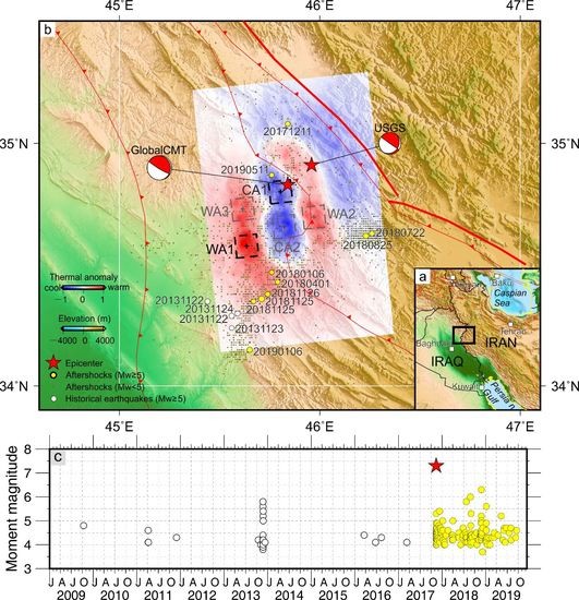
2. Setting and Data
3. Method
3.1. THM Coupled Simulation Method
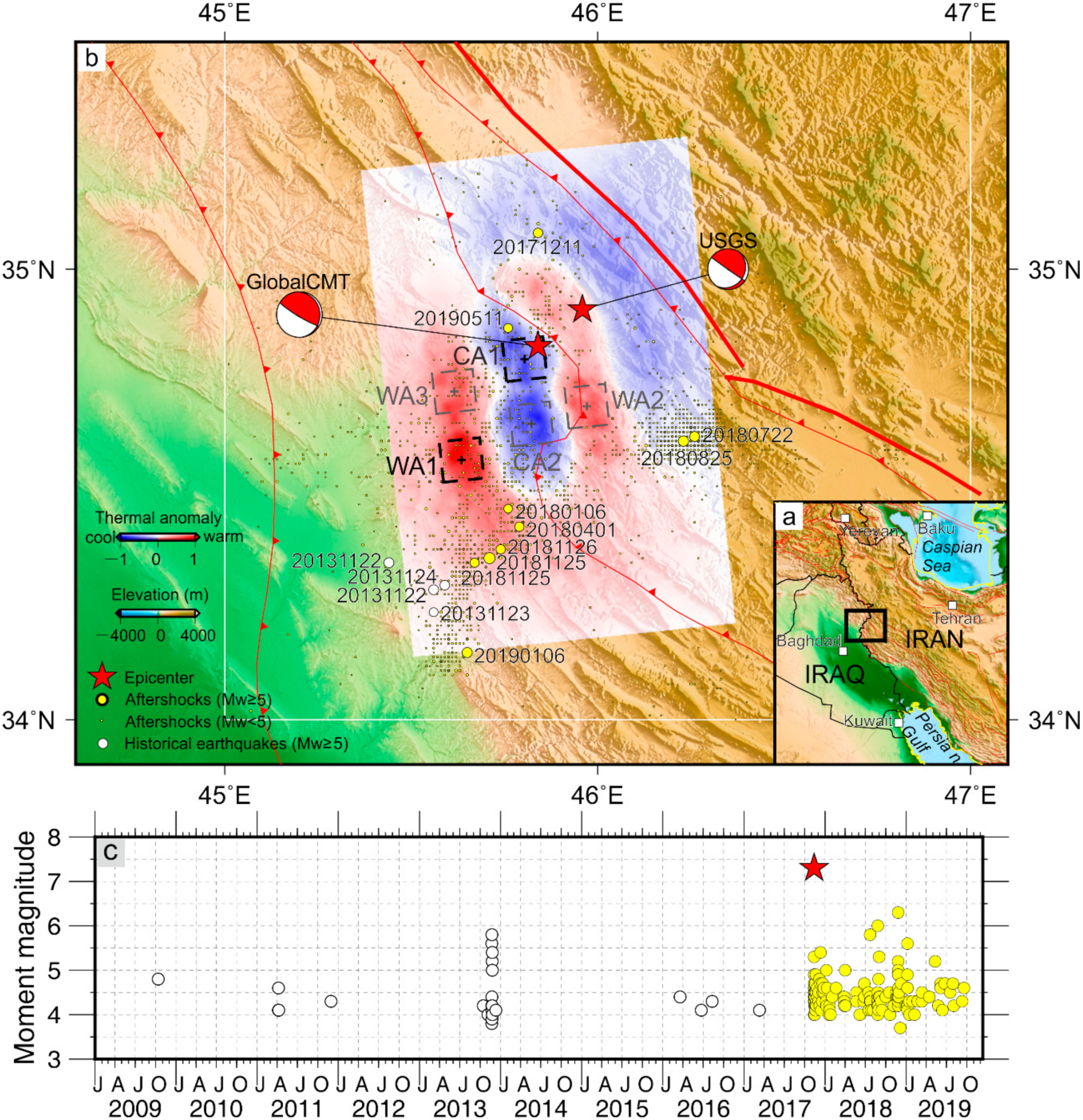
3.2. Attenuation Function Fitting of Nighttime LST Data
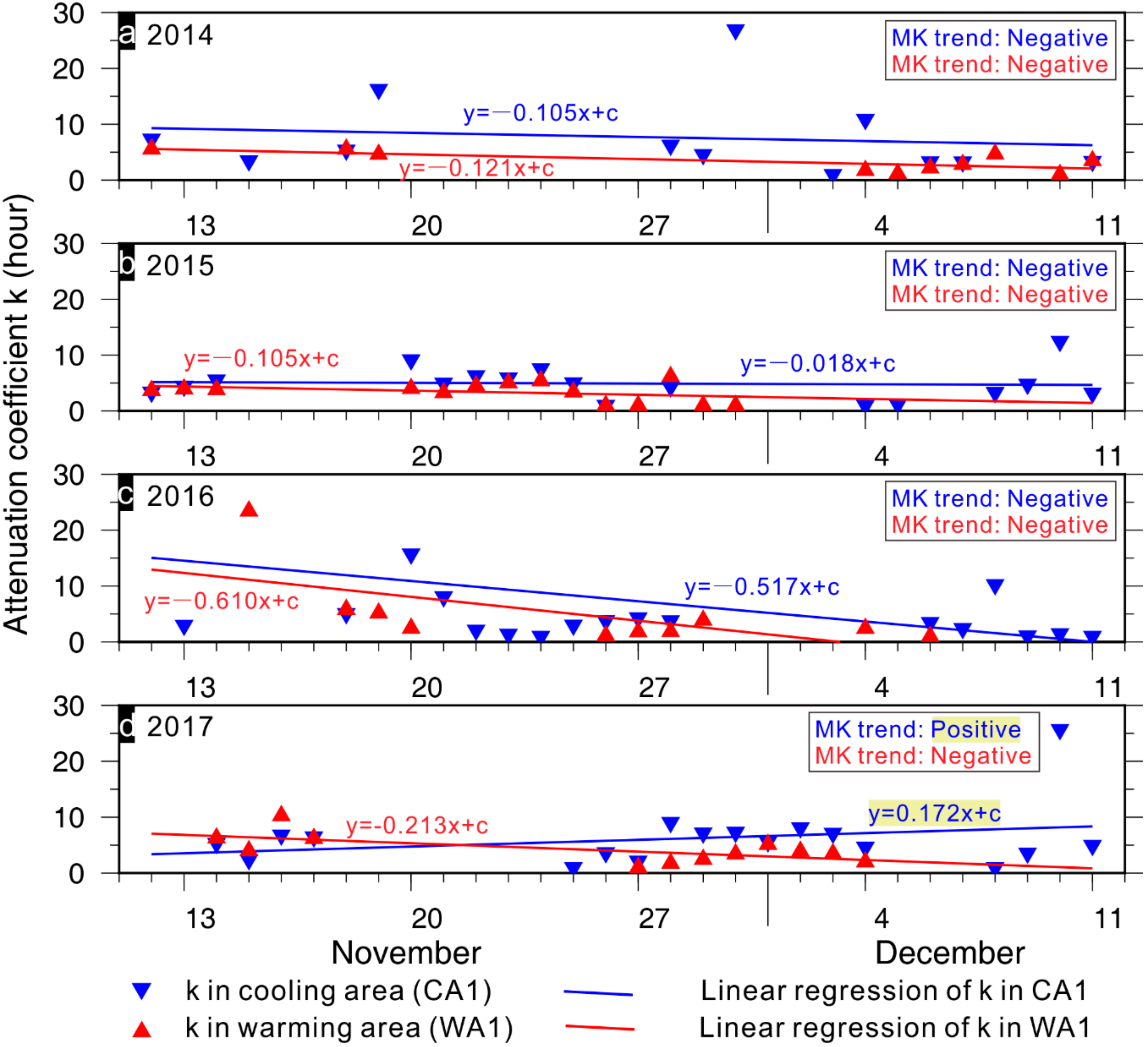
3.3. Attenuation Coefficient Time Series Trends Analysis
3.3.1. Mann–Kendall Trend Test
3.3.2. Sen’s Slope Estimator
4. Results
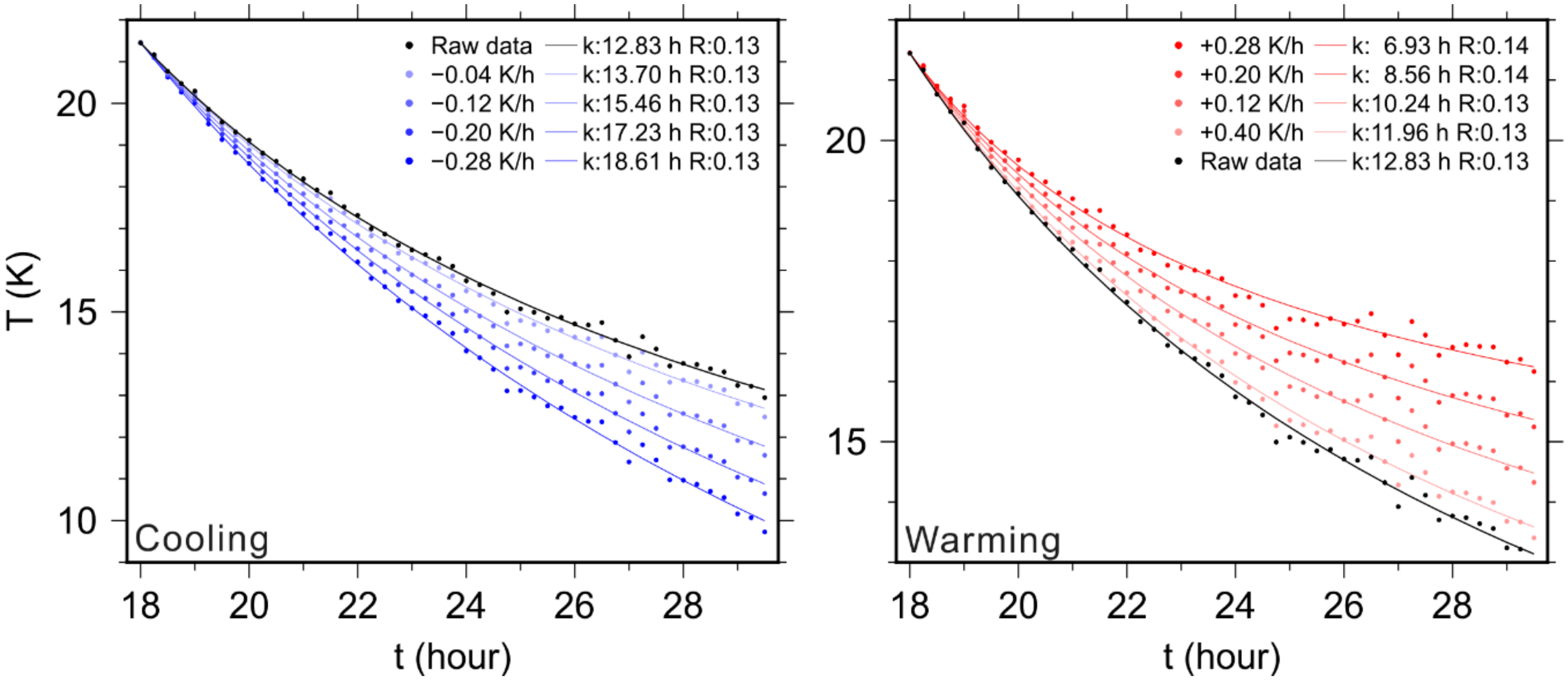
4.1. Co-Seismic Slip-Induced Surface Thermal Variation
4.2. LST Attention Intensity Trend Analysis
5. Discussion
5.1. Reliability Analysis of k Trends
5.2. Seismic Thermal Anomaly Mechanism
5.3. Effect of Afterslip on LST Change
5.4. Limitations
6. Conclusions
Supplementary Materials
Author Contributions
Funding
Acknowledgments
Conflicts of Interest
References
- Sibson, R.H. Interactions between Temperature and Pore-Fluid Pressure during Earthquake Faulting and a Mechanism for Partial or Total Stress Relief. Nat. Phys. Sci. 1973, 243, 66–68. [Google Scholar] [CrossRef]
- Lachenbruch, A.H. Frictional heating, fluid pressure, and the resistance to fault motion. J. Geophys. Res. Space Phys. 1980, 85, 6097–6112. [Google Scholar] [CrossRef]
- Noda, H. Thermal Pressurization and Slip-Weakening Distance of a Fault: An Example of the Hanaore Fault, Southwest Japan. Bull. Seism. Soc. Am. 2005, 95, 1224–1233. [Google Scholar] [CrossRef]
- Talwani, P.; Acree, S. Pore Pressure Diffusion and the Mechanism of Reservoir-Induced Seismicity. In Earthquake Prediction; Birkhäuser: Basel, Switzerland; Boston, MA, USA, 1985; Volume 122, pp. 947–965. [Google Scholar]
- Ellsworth, W.L. Injection-induced earthquakes. Science 2013, 341, 1225942. [Google Scholar] [CrossRef] [PubMed]
- Nur, A.; Booker, J.R. Aftershocks Caused by Pore Fluid Flow? Science 1972, 175, 885–887. [Google Scholar] [CrossRef]
- Segall, P.; Rice, J.R. Does shear heating of pore fluid contribute to earthquake nucleation? J. Geophys. Res. Space Phys. 2006, 111, 09316. [Google Scholar] [CrossRef]
- Rice, J.R. Heating and weakening of faults during earthquake slip. J. Geophys. Res. Space Phys. 2006, 111, 05311. [Google Scholar] [CrossRef]
- Peltzer, G.; Rosen, P.; Rogez, F.; Hudnut, K. Poroelastic rebound along the Landers 1992 earthquake surface rupture. J. Geophys. Res. Space Phys. 1998, 103, 30131–30145. [Google Scholar] [CrossRef]
- Jónsson, S.; Segall, P.; Pedersen, R.; Björnsson, G. Post-earthquake ground movements correlated to pore-pressure transients. Nature 2003, 424, 179–183. [Google Scholar] [CrossRef]
- Sibson, R.H. Fault zone models, heat flow, and the depth distribution of earthquakes in the continental crust of the United States. Bull. Seismol. Soc. Am. 1982, 72, 151–163. [Google Scholar]
- Chen, W.-P.; Molnar, P. Focal depths of intracontinental and intraplate earthquakes and their implications for the thermal and mechanical properties of the lithosphere. J. Geophys. Res. Space Phys. 1983, 88, 4183–4214. [Google Scholar] [CrossRef]
- Kudo, T.; Tanaka, T.; Furumoto, M. Estimation of the Maximum Earthquake Magnitude from the Geothermal Gradient. Bull. Seismol. Soc. Am. 2009, 99, 396–399. [Google Scholar] [CrossRef]
- Lachenbruch, A.H.; Sass, J.H. Heat flow in the United States and the thermal regime of the crust. Earth Crust 1977, 20, 626–675. [Google Scholar]
- Sorey, M.L.; Lewis, R.E. Convective heat flow from hot springs in the Long Valley Caldera, Mono County, California. J. Geophys. Res. Space Phys. 1976, 81, 785–791. [Google Scholar] [CrossRef]
- Wang, Y. Heat flow pattern and lateral variations of lithosphere strength in China mainland: Constraints on active deformation. Phys. Earth Planet. Inter. 2001, 126, 121–146. [Google Scholar] [CrossRef]
- Jing, L.; Feng, X. Numerical modeling for coupled thermo-hydro-mechanical and chemical processes (thmc) of geological media—International and Chinese experiences. Chin. J. Rock Mech. Eng. 2003, 22, 125–136. [Google Scholar]
- Gaucher, E.; Schoenball, M.; Heidbach, O.; Zang, A.; Fokker, P.A.; Van Wees, J.-D.; Kohl, T. Induced seismicity in geothermal reservoirs: A review of forecasting approaches. Renew. Sustain. Energy Rev. 2015, 52, 1473–1490. [Google Scholar] [CrossRef]
- Rattez, H.; Stefanou, I.; Sulem, J.; Veveakis, M.; Poulet, T. The importance of Thermo-Hydro-Mechanical couplings and microstructure to strain localization in 3D continua with application to seismic faults. Part I: Theory and linear stability analysis. J. Mech. Phys. Solids 2018, 115, 54–76. [Google Scholar] [CrossRef]
- Ouzounov, D.; Freund, F. Mid-infrared emission prior to strong earthquakes analyzed by remote sensing data. Adv. Space Res. 2004, 33, 268–273. [Google Scholar] [CrossRef]
- Panda, S.K.; Choudhury, S.; Saraf, A.K.; Das, J.D. MODIS land surface temperature data detects thermal anomaly preceding 8 October 2005 Kashmir earthquake. Int. J. Remote Sens. 2007, 28, 4587–4596. [Google Scholar] [CrossRef]
- Blackett, M.; Wooster, M.J.; Malamud, B.D. Exploring land surface temperature earthquake precursors: A focus on the Gujarat (India) earthquake of 2001. Geophys. Res. Lett. 2011, 38, 15303. [Google Scholar] [CrossRef]
- Zoran, M. MODIS and NOAA-AVHRR l and surface temperature data detect a thermal anomaly preceding the 11 March 2011 Tohoku earthquake. Int. J. Remote Sens. 2012, 33, 6805–6817. [Google Scholar] [CrossRef]
- Qiang, Z.; Xu, X.; Lin, C. Thermal Infrared anomaly—Precursor of impending earthquakes. Chin. Sci. Bull. 1991, 36, 319–323. [Google Scholar] [CrossRef]
- Tronin, A.A.; Hayakawa, M.; Molchanov, O.A. Thermal IR satellite data application for earthquake research in Japan and China. J. Geodyn. 2002, 33, 519–534. [Google Scholar] [CrossRef]
- Bhardwaj, A.; Singh, S.; Sam, L.; Joshi, P.; Bhardwaj, A.; Martín-Torres, F.J.; Kumar, R. A review on remotely sensed land surface temperature anomaly as an earthquake precursor. Int. J. Appl. Earth Obs. Geoinf. 2017, 63, 158–166. [Google Scholar] [CrossRef]
- Jiao, Z.-H.; Zhao, J.; Shan, X. Pre-seismic anomalies from optical satellite observations: A review. Nat. Hazards Earth Syst. Sci. 2018, 18, 1013–1036. [Google Scholar] [CrossRef]
- Lisowski, M.; Prescott, W.H.; Savage, J.C.; Johnston, M.J. Geodetic estimate of coseismic slip during the 1989 Loma Prieta, California, Earthquake. Geophys. Res. Lett. 1990, 17, 1437–1440. [Google Scholar] [CrossRef]
- Simons, M.; Fialko, Y.; Rivera, L. Coseismic deformation from the 1999 M w 7.1 Hector Mine, California, earthquake as inferred from InSAR and GPS observations. Bull. Seismol. Soc. Am. 2002, 92, 1390–1402. [Google Scholar] [CrossRef]
- Biot, M.A. Mechanics of Deformation and Acoustic Propagation in Porous Media. J. Appl. Phys. 1962, 33, 1482–1498. [Google Scholar] [CrossRef]
- Bear, J.; Bachmat, Y. Introduction to Modeling of Transport Phenomena in Porous Media. Theory Appl. Trans. Porous Media 1990, 4, 481–516. [Google Scholar]
- Nield, D.A.; Bejan, A. Convection in Porous Media; Springer: Berlin, Germany, 2013; Volume 108, pp. 284–290. [Google Scholar]
- Inamdar, A.K.; French, A.; Hook, S.; Vaughan, G.; Luckett, W. Land surface temperature retrieval at high spatial and temporal resolutions over the southwestern United States. J. Geophys. Res. Space Phys. 2008, 113, 07107. [Google Scholar] [CrossRef]
- Sun, D.; Pinker, R.T.; Kafatos, M. Diurnal temperature range over the United States: A satellite view. Geophys. Res. Lett. 2006, 33, 05705. [Google Scholar] [CrossRef]
- Duan, S.-B.; Li, Z.-L.; Tang, B.-H.; Wu, H.; Tang, R.; Bi, Y.; Zhou, G. Estimation of Diurnal Cycle of Land Surface Temperature at High Temporal and Spatial Resolution from Clear-Sky MODIS Data. Remote Sens. 2014, 6, 3247. [Google Scholar] [CrossRef]
- Piroddi, L.; Ranieri, G. Night thermal gradient: A new potential tool for earthquake precursors studies. An application to the seismic area of L’Aquila (central Italy). IEEE J. Sel. Top. Appl. Earth. Obs. Remote Sens. 2012, 5, 307–312. [Google Scholar] [CrossRef]
- Trigo, I.F.; Monteiro, I.T.; Olesen, F.; Kabsch, E. An assessment of remotely sensed land surface temperature. J. Geophys. Res. Space Phys. 2008, 113, 17108. [Google Scholar] [CrossRef]
- United States Geological Survey. Available online: https://www.usgs.gov/ (accessed on 4 September 2019).
- Ahmadi, A.; Bazargan-Hejazi, S. 2017 Kermanshah Earthquake: Lessons Learned. J. Inj. Violence Res. 2018, 10, 1–2. [Google Scholar]
- Chen, K.; Xu, W.; Mai, P.; Gao, H.; Zhang, L.; Ding, X. The 2017 Mw 7.3 Sarpol Zahāb Earthquake, Iran: A compact blind shallow-dipping thrust event in the mountain front fault basement. Tectonophysics 2018, 747, 108–114. [Google Scholar] [CrossRef]
- Gutenberg, B.; Richter, C.F. Earthquake magnitude, intensity, energy, and acceleration: (Second paper). Bull. Seismol. Soc. Am. 1956, 46, 105–145. [Google Scholar]
- Wan, Z.; Dozier, J. A generalized split-window algorithm for retrieving land-surface temperature from space. IEEE Trans. Geosci. Remote Sens. 1996, 34, 892–905. [Google Scholar]
- Bear, J.; Bachmat, Y. Introduction to modeling of transport phenomena in porous media. In Theory & Applications of Transport in Porous Media; Springer Science & Business Media: London, UK, 2012; Volume 4, pp. 481–516. [Google Scholar]
- Göttsche, F.-M.; Olesen, F.S. Modelling of diurnal cycles of brightness temperature extracted from METEOSAT data. Remote Sens. Environ. 2001, 76, 337–348. [Google Scholar] [CrossRef]
- Gocic, M.; Trajkovic, S. Analysis of changes in meteorological variables using Mann-Kendall and Sen’s slope estimator statistical tests in Serbia. Glob. Planet. Chang. 2013, 100, 172–182. [Google Scholar] [CrossRef]
- Mann, H.B. Nonparametric tests against trend. Econometrica 1945, 13, 245–259. [Google Scholar] [CrossRef]
- Kendall, K. Thin-film peeling-the elastic term. J. Phys. D 1975, 8, 1449. [Google Scholar] [CrossRef]
- Sen, P.K. Estimates of the regression coefficient based on Kendall’s tau. J. Am. Stat. Assoc. 1968, 63, 1379–1389. [Google Scholar] [CrossRef]
- Feng, W.; Samsonov, S.; Almeida, R.; Yassaghi, A.; Li, J.; Qiu, Q.; Li, P.; Zheng, W. Geodetic Constraints of the 2017 Mw7. 3 Sarpol Zahab, Iran Earthquake, and Its Implications on the Structure and Mechanics of the Northwest Zagros Thrust-Fold Belt. Geophys. Res. Lett. 2018, 45, 6853–6861. [Google Scholar] [CrossRef]
- Akhoondzadeh, M.; De Santis, A.; Marchetti, D.; Piscini, A.; Jin, S. Anomalous seismo-LAI variations potentially associated with the 2017 Mw=7.3 Sarpol-e Zahab (Iran) earthquake from Swarm satellites, GPS-TEC and climatological data. Adv. Space Res. 2019, 64, 143–158. [Google Scholar] [CrossRef]
- Wu, L.; Zhou, Y.; Miao, Z.; Qin, K. Anomaly Identification and Validation for Winter 2017 Iraq and Iran Earthquakes. In Proceedings of the 20th EGU General Assembly, EGU2018, Vienna, Austria, 4–13 April 2018; Volume 20, p. 5800. [Google Scholar]
- Tse, S.T.; Rice, J.R. Crustal earthquake instability in relation to the depth variation of frictional slip properties. J. Geophys. Res. Space Phys. 1986, 91, 9452–9472. [Google Scholar] [CrossRef]


| Areas | Time | Reg. (h/d) | Zs | Qmed |
|---|---|---|---|---|
| WA1 | 2014 | −0.166 | −1.868 | −0.545 |
| 2015 | −0.105 | −0.766 | −0.125 | |
| 2016 | −0.610 | −2.147 | −0.602 | |
| 2017 | −0.213 | −1.166 | −0.270 | |
| CA1 | 2014 | −0.105 | −1.166 | −0.267 |
| 2015 | −0.018 | −0.865 | −0.102 | |
| 2016 | −0.517 | −2.239 | −0.353 | |
| 2017 | 0.172 | 0.530 | 0.085 |
© 2019 by the authors. Licensee MDPI, Basel, Switzerland. This article is an open access article distributed under the terms and conditions of the Creative Commons Attribution (CC BY) license (http://creativecommons.org/licenses/by/4.0/).
Share and Cite
Zhu, C.; Jiao, Z.; Shan, X.; Zhang, G.; Li, Y. Land Surface Temperature Variation Following the 2017 Mw 7.3 Iran Earthquake. Remote Sens. 2019, 11, 2411. https://doi.org/10.3390/rs11202411
Zhu C, Jiao Z, Shan X, Zhang G, Li Y. Land Surface Temperature Variation Following the 2017 Mw 7.3 Iran Earthquake. Remote Sensing. 2019; 11(20):2411. https://doi.org/10.3390/rs11202411
Chicago/Turabian StyleZhu, Chuanhua, Zhonghu Jiao, Xinjian Shan, Guohong Zhang, and Yanchuan Li. 2019. "Land Surface Temperature Variation Following the 2017 Mw 7.3 Iran Earthquake" Remote Sensing 11, no. 20: 2411. https://doi.org/10.3390/rs11202411
APA StyleZhu, C., Jiao, Z., Shan, X., Zhang, G., & Li, Y. (2019). Land Surface Temperature Variation Following the 2017 Mw 7.3 Iran Earthquake. Remote Sensing, 11(20), 2411. https://doi.org/10.3390/rs11202411