1. Introduction
Object detection in high resolution optical remote sensing images is to determine if a given aerial or satellite image contains one or more objects belonging to the class of user focused and locate the position of each predicted object in the image [
1]. As an important research topic of remote sensing images analysis, object detection in remote sensing images is widely applied to military reconnaissance, intelligent transportation, urban planning, and other domains [
2,
3,
4,
5]. In recent years, with the development of optical remote sensing technology and space-borne intelligent information processing system, it is a trend to construct a system that combines remote sensing detection with information processing on satellite or aircraft. Efficient object detection in a remote sensing image and processing on a satellite or aircraft can not only reduce the amount of communication data, but also achieve efficient, flexible, and fast earth observation tasks. However, there are many challenges to detect the user-concerned objects quickly and accurately from the massive remote sensing data. Firstly, remote sensing images have ultra-high spatial resolution, which usually contains tens or hundreds of millions of pixels. Quickly and accurately detecting the user-focused objects from massive amounts of data is a challenging task. Secondly, objects in remote sensing images have multi-scale features. For example, objects such as a ground track field, bridge, etc. have hundreds of pixels, while small objects such as a vehicle, ship, etc. may only contain a few pixels. This feature makes accurate object detection in remote sensing images more difficult, especially for small objects. Thirdly, objects in a remote sensing image viewed from overhead have any orientation, while natural image sets are typically acquired horizontally. Therefore, models trained on natural image sets cannot be directly applied to remote sensing image object detection. In addition, the general-purpose processor that carries out the algorithm cannot meet the requirements of space-borne or airborne information processing with high performance and low energy consumption. Therefore, the design of efficient object detection algorithm framework and hardware architecture for remote sensing images has become an urgent problem to be solved for space-borne or airborne information processing.
There are many methods for object detection in remote sensing images after years of research and development. We summarize these methods into traditional object detection methods based on prior information and manual features and deep learning based object detection methods. The traditional object detection methods based on prior information and manual designed features regard object detection as a classification problem composed of feature extraction and object classification, which includes template matching-based object detection methods, knowledge-based object detection methods, object-based image analysis-based (OBIA-based) object detection methods, and machine learning object detection methods based on prior information and manual designed features [
1]. The template matching-based object detection methods are divided into two steps. Firstly, the template is trained from existing data by hand-crafting or statistical methods, and then the similarity measurement is performed on the pre-processed input image to complete the detection. The template matching-based object detection approaches are usually divided into a rigid template and deformable template according to the template type selected by the user [
1,
6,
7]. The knowledge-based object detection methods setup knowledge and rules based on geometric information and context information, and generate hypotheses on the input image and convert the object detection problem into a hypothesis testing problem [
8,
9,
10]. The OBIA-based object detection methods accomplish the detection task by segmenting the input image and classifying the object, wherein the scale of the image segmentation directly affects the detection result [
11,
12,
13]. The machine learning object detection methods based on prior information and manual designed features are typically divided into two stages: feature extraction stage and object classification and recognition stage. In the feature extraction stage, selective search is usually used to extract handcrafted features, such as scale-invariant feature transform (SIFT) [
14], histogram of oriented gradients (HOG) [
15], bag-of-words (BoW) feature [
16], texture features [
17], and so on. In the stage of object classification and recognition, classifiers often include: support vector machine (SVM) [
18], AdaBoost [
19], deformable parts model (DPM) [
20], condition random field (CRF) [
21], sparse coding-based classifier [
22] and artificial neural network (ANN) [
23], and so on. However most of these methods mentioned above rely on the prior information and manual designed features, and it is difficult to efficiently achieve object detection tasks under massive remote sensing data.
In recent years, deep learning technology has achieved great success in computer vision applications, and the deep learning based object detection methods have become the mainstream in the field of image recognition. The deep convolutional neural network AlexNet proposed by Krizhevsky, A. et al. not only won the 2012 ImageNet Large Scale Visual Recognition Challenge (ILSVR 2012), but also set off a wave of deep learning research [
24]. Since then, many researchers have proposed a variety of excellent deep learning algorithms, and deep convolutional neural networks have become the best deep learning algorithm in the field of image recognition. Researchers have also begun to apply deep learning technology to object recognition in remote sensing images. For example, Cheng, G. et al. applied the rotation-invariant convolutional neural networks (RICNN) to object detection in very high resolution (VHR) optical remote sensing images [
25]. Wang, G. et al. proposed the infrastructure target detection of remote sensing image based on residual networks [
26]. Although these object detection methods based on convolutional neural networks perform well in remote sensing image object detection, they do not form a unified and efficient object framework. Currently, the deep learning object detection algorithm framework based on convolutional neural network has made great progress. These mainstream algorithm frameworks include region proposal-based two-stage object detection algorithm and regression-based one stage object detection algorithm [
27]. The region proposal-based algorithm generates a series of region proposals according to selective search (SS), Bing or edge boxes methods firstly, and then extracts the features by the deep neural networks, and implements object classification and boundary regression based on these features. For example, Girshick, R. et al. proposed region-based convolutional neural networks (R-CNN) [
28], which combines object candidate regions and deep learning for object detection. Then he proposed the more efficient fast R-CNN algorithm [
29], which overcomes the shortcomings of R-CNN’s redundant operation when extracting features. Subsequently, Ren, S. et al. proposed a faster R-CNN algorithm [
30], which uses region proposal networks (RPN) to extract object candidate regions, and integrates the entire object candidate region extraction, feature extraction, object recognition, and detection into a deep neural network framework. In order to solve the multi-scale detection problem, Lin, T.Y. et al. introduced the feature pyramid network (FPN) to improve the recognition efficiency of small objects [
31]. However, the object detection algorithm framework based on the region proposal is not very efficient because it takes more time to extract the candidate region. The regression-based object detection algorithm has no candidate region extraction step, which combines all recognition and detection steps in a deep neural network, and has high detection and recognition efficiency. For this type of algorithm framework, the you only look once (YOLO) algorithm framework proposed by Redmon, J. et al. requires only a single network to evaluate the entire image to obtain the target bounding box and category [
32]. The single shot multi-box detector (SSD) algorithm framework proposed by Liu, W. et al. introduces an anchor mechanism based on YOLO, which detects the object on the different scales and improves accuracy without affecting process speed [
33]. In general, the deep learning based object detection methods have made great progress in the accuracy and efficiency of object detection compared to the traditional methods. At present, these algorithms are widely used in remote sensing image object detection. However, these algorithms are not satisfactory for the detection of small objects in the images, and they need to be improved. Meanwhile, for the airborne or space-borne application environment, not only the object detection accuracy but also the computation complexity and model size need to be considered.
The rapid development of deep learning technology is inseparable from the support of high performance hardware computing systems. The performance of deep learning algorithms is not only related to its own structure, but also depends on the hardware architecture of computing system that carries out the algorithm. Currently, the training and inference of deep learning algorithms mainly depends on general-purpose processors, such as central processing units (CPUs) and graphics processing units (GPUs). Although the general-purpose CPUs have higher flexibility and better parallel computing power, the deep learning algorithm does not achieve better execution efficiency. GPUs are widely used in training and inference of deep learning algorithms because of its unique many-core architecture and superior parallel computing power, but it cannot obtain good performance-power ratio due to high power consumption. In some specific applications, not only high processing performance but also stricter power consumption requirements are required. For example, in embedded application scenarios or on satellite or aircraft information processing systems, general-purpose CPUs and GPUs will not be able to accommodate the application requirements in such situations. Therefore, application-oriented domain-specific architecture (DSA) is the solution to overcome such problems currently [
34]. In recent years, many researchers have proposed different hardware architectures for their respective application scenarios. Farabet, C. et al. proposed CNP [
35] with parallel vector computing architecture for low-power lightweight unmanned aircraft vehicles (UAVs) or robots, and a scalable dataflow 2-D grid hardware architecture Neuflow [
36] optimized for the computation of general-purpose vision algorithms. Peemem, M. et al. proposed hierarchical memory-centric accelerator architecture to improve the performance of convolutional operations and reduce the overhead of memory access [
37]. Alwani, M. et al. reduced the transfer of off-chip feature map data by modifying the order of input data and fusing multiple continuous convolutional layer processing [
38]. Chen, T. et al. presented a high-throughput algorithm accelerator DianNao based on adder tree structure for large-scale convolutional neural network (CNN) and deep neural network (DNN) [
39]. Du, Z. et al. proposed ShiDianNao based on 2-D mesh topology structure for image recognition applications near to sensors, and reduced memory usage through weight sharing [
40]. Zhang, C. et al. designed a CNN accelerator based on the adder tree structure by quantitative analysis of memory bandwidth required for throughput [
41]. Google has introduced a high-performance tensor processing unit (TPU) for data centers based on 2-D systolic array architecture [
42]. Li, L. et al. designed a co-processor with 2-D mesh topology structure for image recognition by optimization calculation of algorithm [
43]. Chang, J.W. et al. proposed a deconvolutional neural networks accelerator (DCNN) with 2-D mesh architecture for super-resolution images [
44]. These hardware architectures are designed for a specific application scenario and are mainly used to accelerate the calculation of the deep learning algorithms. The processing elements (PEs) in these processors are typically organized in 1-D or 2-D topology structure. These processors only implement parallel computation of synapses and neurons, which compute each feature map one by one. However, the feature map in the image object detection is 3-D, but the current design do not consider the parallel calculation of feature map, so there is still potential for mining parallelism. Meanwhile, the storage organization and data reuse need to be considered in the architecture to adapt to large-scale algorithms and parameters, which is very important for computing and storage dual-intensive remote sensing images object detection applications.
In order to adapt to the characteristics of object detection in remote sensing images and tackle the problems of the algorithm framework and hardware architecture mentioned above, we propose an efficient context-based feature fusion SSD (CBFF-SSD) algorithm framework. Subsequently, we have designed hardware architecture of deep learning processor with multiple 2-D mesh architecture supporting feature maps parallel processing by analyzing and optimizing the calculation of each layer in the deep learning algorithm framework. Finally, the efficiency and performance of the algorithm framework and processor are evaluated by multiple experiments and indicators. The main contributions of this paper are summarized as follows:
We propose a context-based feature fusion SSD (CBFF-SSD) framework for object detection in remote sensing images. MobileNet is used as the backbone network in the algorithm framework to reduce the amount of calculation and parameters, which makes the algorithm more efficient. Two feature fusion units and seven feature maps are used in the algorithm to enhance the detection of multi-scale objects and small objects, and improve the detection accuracy.
We analyze and optimize the calculation of each layer in the algorithm framework, which makes it easy to implement in hardware, and lays a foundation for the design of time-division multiplexing processing unit in the subsequent hardware architecture of deep learning processor.
We propose efficient hardware architecture of deep learning processor with multiple 2-D mesh topology oriented to image object recognition, which can simultaneously calculate multiple output feature maps. Hierarchical on-chip storage organization makes the neurons and weights to be efficiently delivered to the neural processing units (NPUs). The parallel architecture, the hierarchical storage organization, and the register designed in the PE effectively realize the sharing and reuse of the calculation data.
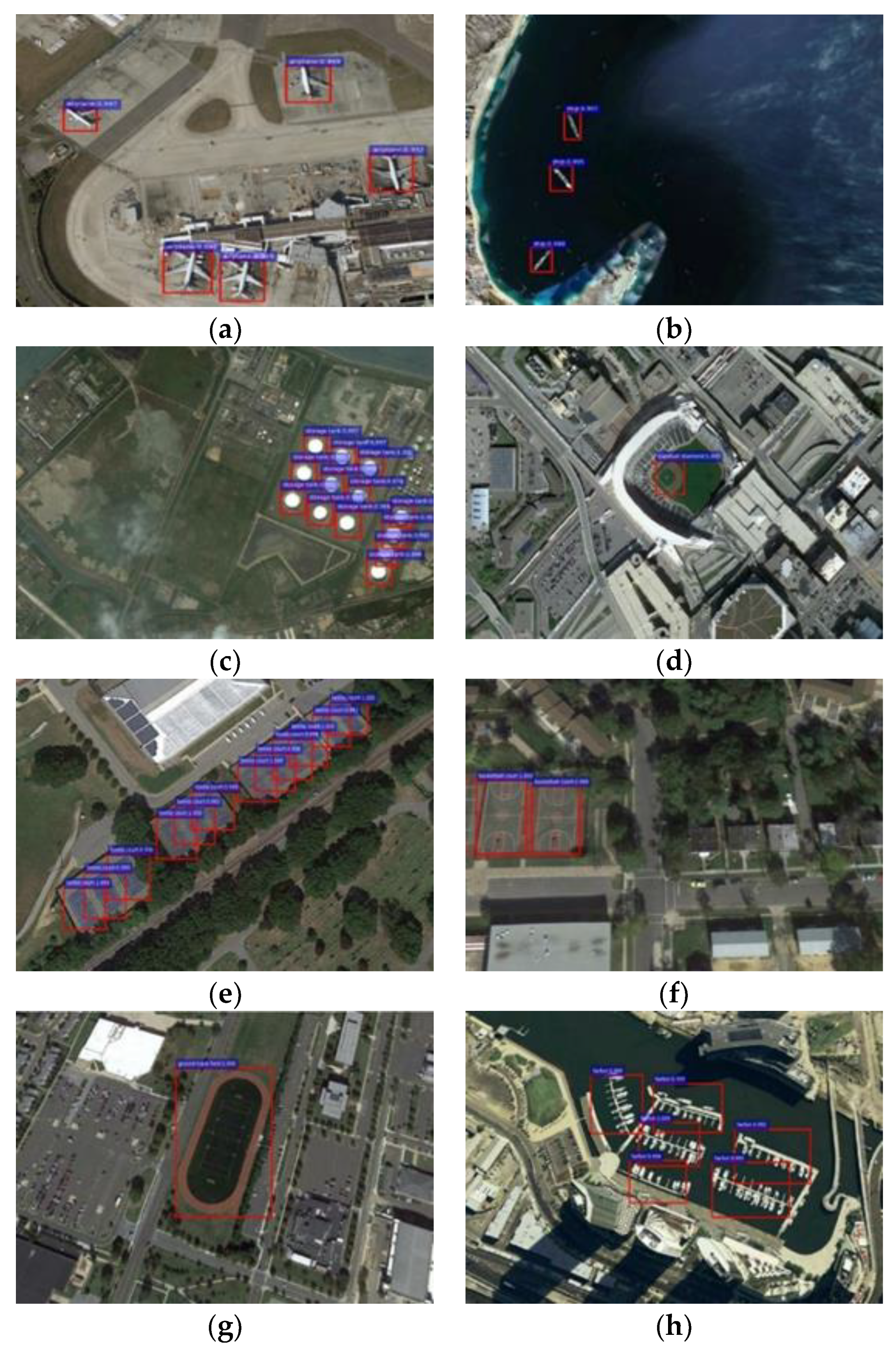
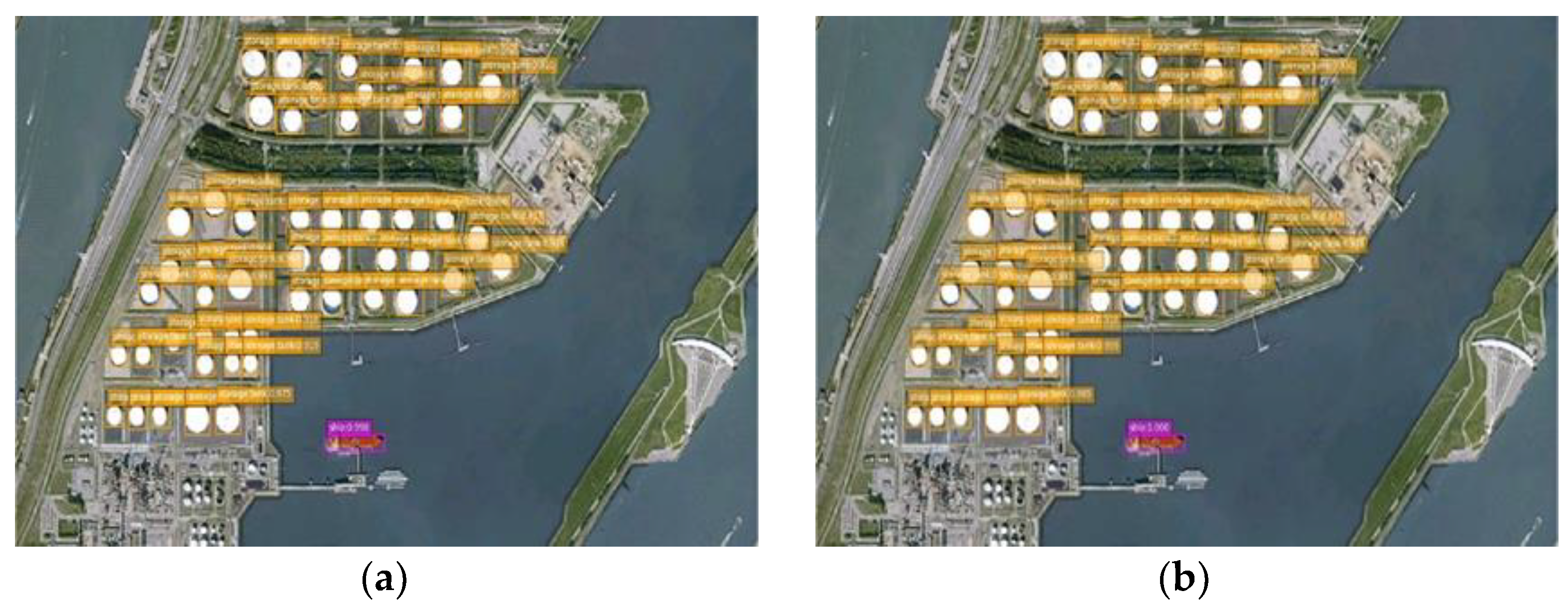
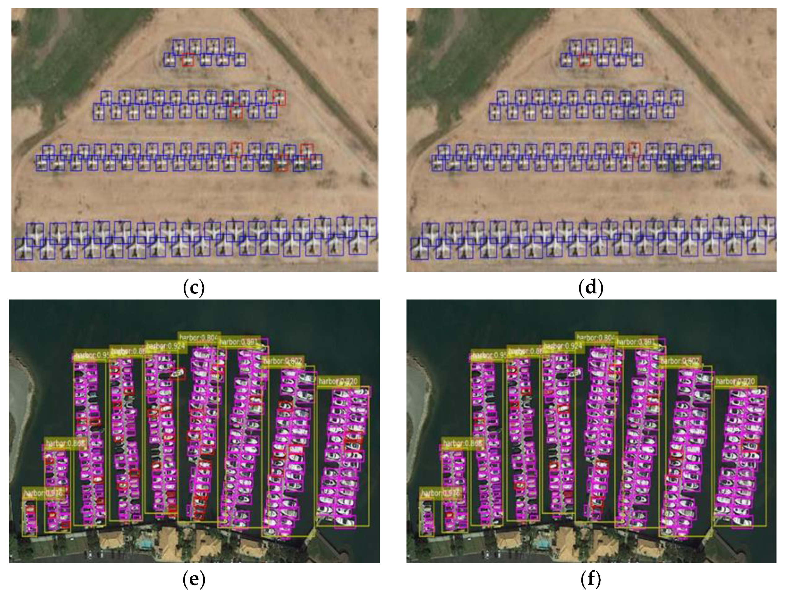
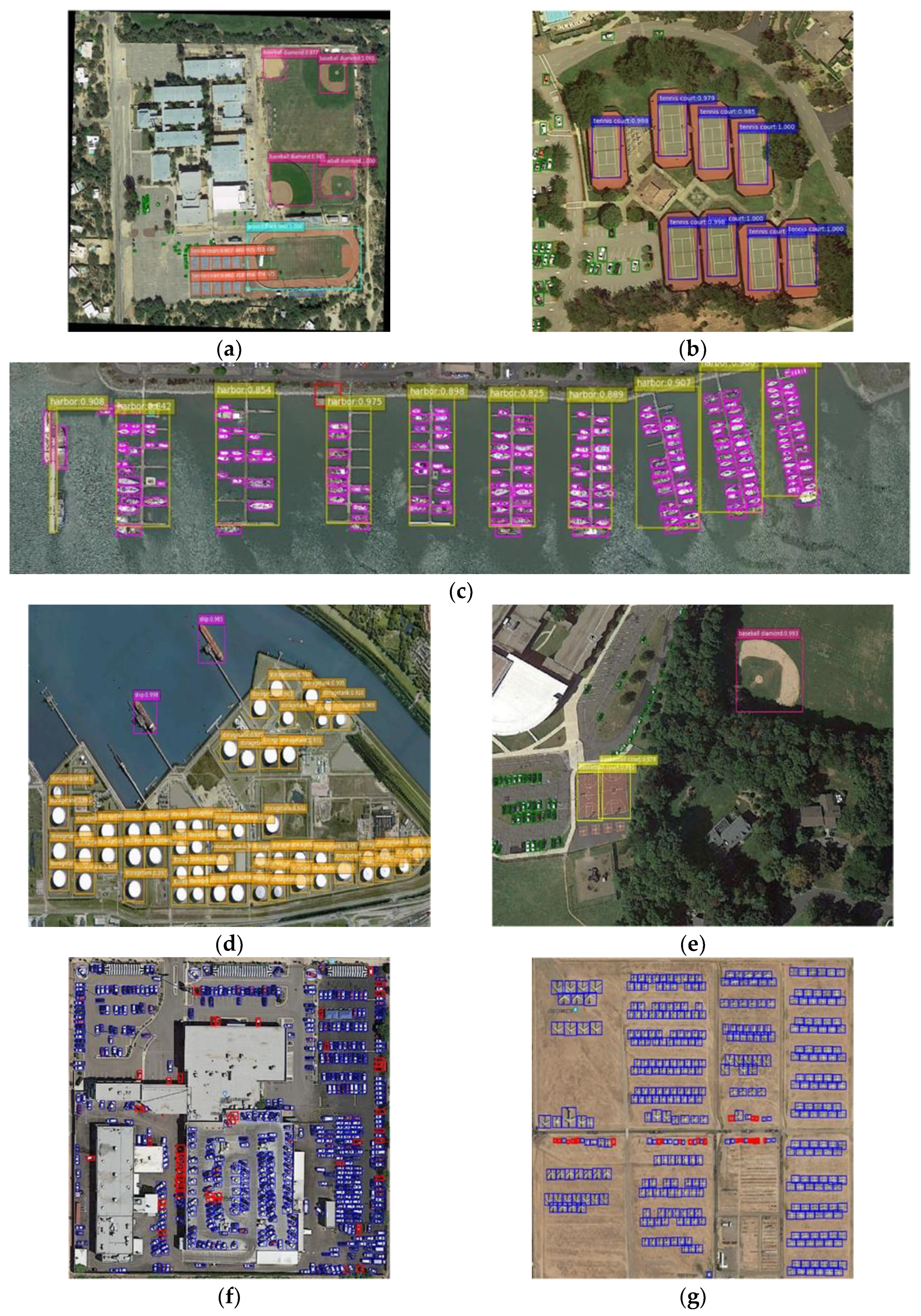
We evaluate the performance and efficiency of the algorithm framework and hardware architecture based on several experiments and evaluation indicators. The performance of the proposed algorithm framework is compared with the several popular algorithms on the NWPU-VHR-10 dataset. We realize the proposed hardware architecture of the deep learning processor on the field programmable gate array (FPGA), and then evaluate the processing performance and compared with the CPU, GPU, and the current popular deep learning processors. The experimental results confirmed the effectiveness and superiority of the proposed algorithm framework and hardware architecture of deep learning processor.
The rest of this paper is organized as follows.
Section 2 proposes the context-based feature fusion SSD (CBFF-SSD) framework. The calculation of each layer in deep learning algorithm framework and optimization are described in
Section 3.
Section 4 introduces the details of the hardware architecture of deep learning processor.
Section 5 presents the experimental results and analysis. The experimental results are discussed in the
Section 6. Finally, the conclusions are drawn in
Section 7.
2. Context-Based Feature Fusion SSD Framework
2.1. Related Works
The deep learning algorithm based on the convolutional neural network model has achieved excellent results in image object detection applications, which not only improves the accuracy of recognition, but also improves the efficiency of recognition. In particular, the recent rapid development of the region proposal-based objects detection algorithm framework and the regression-based objects detection algorithm framework are particularly outstanding. Since remote sensing images have ultra-high resolution, diverse object sizes and directions, including small targets, and diverse shooting angles, it is full of challenges to quickly and accurately detect the user-focused object from massive remote sensing data. For the application of remote sensing image object detection, many researchers have conducted a lot of research based on the two popular algorithm frameworks.
For examples, Han, X. et al. proposed a highly efficient and robust integrated geospatial object detect framework based on the faster region-based convolutional neural network (Faster R-CNN), which realized the integrated procedure by sharing features between the region proposal generation stage and the object detection stage [
45]. Zhu, M. et al. proposed an effective airplane detection method in remote sensing images based on Faster R-CNN and multiplayer feature fusion, which solved the problem of insufficient representation ability of weak and small objects and overlapping detection boxes in airplane object detection [
3]. Etten, A.V. presented a rapid multi-scale object detection method based on YOLO and DarkNet for the detection of small objects in large satellite imagery [
46]. In order to solve the detection of small and dense objects, Zhang, X. et al. proposed an effective region-based VHR remote sensing imagery object detection framework named double multi-scale feature pyramid network (DM-FPN) [
47].
In summary, the above algorithms are improved for the small objects detection in remote sensing images, and have achieved good object detection results. However, efficient on-board remote sensing image object detection not only needs to consider the accuracy of detection, but also needs to think about the efficiency of calculations such as computational complexity and the number of parameters.
2.2. CBFF-SSD Framework
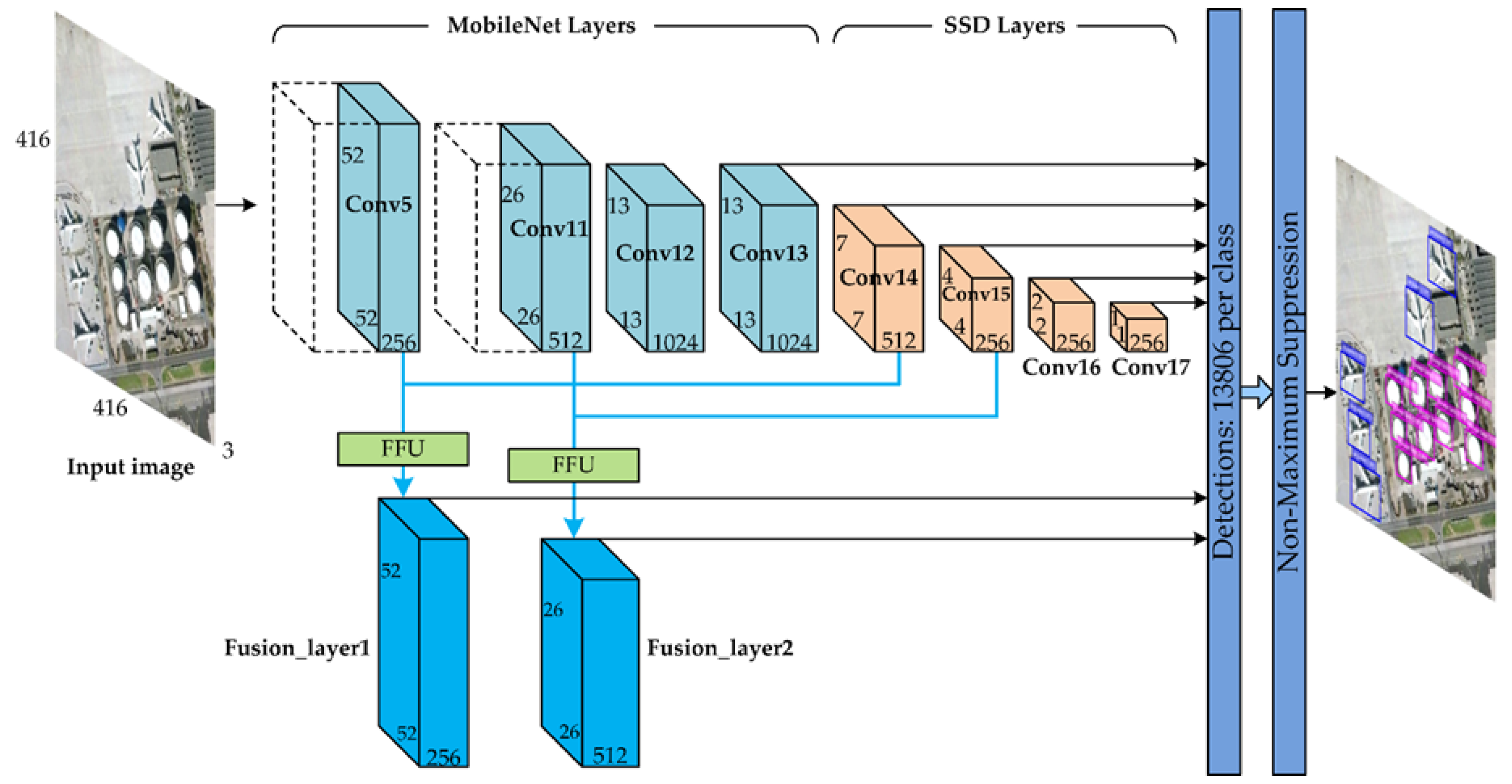
Based on the in-depth analysis of the characteristics and challenges of object detection in a remote sensing image on a satellite or aircraft, we proposed a context-based feature fusion SSD (CBFF-SSD) algorithm framework shown in
Figure 1. The whole algorithm framework was designed based on the SSD framework [
33]. This is because on the one hand, the regression-based object detection framework is considered to be more efficient in image object detection, and the other is because the algorithm framework is more suitable for multi-scale object detection. Different from the SSD framework, the backbone network uses the MobileNet [
48] instead of VGGNet. The lightweight MobileNet uses depth-wise separable convolution to effectively reduce the amount of calculation and parameters of the algorithm, which is more conducive to efficient object detection in embedded applications, especially in a space-borne or airborne application environment. We compared the number of parameters and the amount of calculations of the proposed CBFF-SSD algorithm framework and the SSD algorithm in
Table 1. It can be seen that the number of parameters of the proposed CBFF-SSD algorithm framework was 56.09% of the SSD algorithm, and the calculation amount was only 17.56% of the SSD algorithm. By reducing the size of the model parameters and computational complexity, the proposed algorithm framework was more effective in object detection.
The high-level features of the convolutional network were rich in semantics and suitable for detecting large objects. After layer-by-layer down-sampling, the features lose too much detail information, and it is often important to small object detection. The feature rich in semantic information was mapped back to the lower layer features with larger resolution and richer detail information, and they were fused in an appropriate way to improve the effect of small object detection. Therefore, in the algorithm framework, the low-level feature map Conv5 (52 × 52 × 256) was added, and the Conv14 and Conv15 were respectively up-sampled and fused with Conv5 and Conv11 layers to improve the precision of small object detection.
Figure 1 shows the architecture details of the CBFF-SSD algorithm framework. The Fusion_layer1, Fusion_layer2, Conv13, Conv14, Conv15, Conv16, and Conv17 were used to predict both location and confidences. In the deep learning algorithm, the resolution of the input image and the number of detection boxes for each class of object affected the accuracy of the detection. Based on the SSD framework, we adjusted the input resolution from 300 × 300 to 416 × 416, and increased the number of detection boxes from 8732 to 13806 to ensure the recognition accuracy of the proposed algorithm framework.
2.3. Feature Fusion Unit (FFU)
There are two feature fusion units in the proposed algorithm framework as shown in
Figure 1. The structure of the feature fusion unit is shown in
Figure 2. The design of feature fusion unit is inspired by the design of the deconvolution module in the deconvolutional single shot detector (DSSD) [
49]. The high-level feature maps are processed by deconvolution to the same size and channel as the lower-level feature maps. Then they are fused by element wise addition.
Taking the feature fusion layer 1 as an example, in order to fuse the feature maps of the Conv14 and Conv5, it is necessary to up-sample the resolution of the Conv14 layer by eight times. Specifically, for the Conv14 layer, we designed three deconvolution layers with stride 2 to achieve up-sampling. Since the feature maps in the feature fusion unit are computationally intensive, we also applied depth-wise separable convolutions here to reduce parameters and computational complexity. The deconvolution layer was followed by depth-wise separable convolution. The depth-wise separable convolution was composed of 3 × 3 depth-wise convolutional layer, batch normalization, rectified linear unit (ReLU) layer, 1 × 1 point-wise convolutional layer, batch normalization layer, and ReLU layer. The Conv5 layer underwent a depth-wise separable convolution module. After the normalization layer, we fused them by element-wise addition, and finally passed the ReLU to complete the fusion.
Fusion layer 2 used the same calculation method, and only the channel was adjusted. Only minor modifications were required for models with different input resolutions.
2.4. Training
We used the same training strategy as SSD [
33]. During training, a set of default boxes was matched to the ground truth boxes. For each ground truth box, we matched it to the default box with the Jaccard overlap higher than a threshold (e.g., 0.5). This was more conducive to predicting multiple bounding boxes with high confidence for overlapped objects. We selected the non-matched default boxes with top loss value as the negative samples so that the ratio of negative and positive was 3:1.
The training objective was for multiple object categories. We set
x to be an indicator for matching the default box to the ground truth box of category p, which equaled to 1 or 0. The
c,
l, and
g represent confidences, the predicted box, and ground truth box respectively. The overall objective loss function is a weighted sum of the localization loss
Lloc and the confidence loss
Lconf, which is defined as:
where
N is the number of matched default boxes, and the weight term
α is set to 1 by cross validation. The localization loss
Lloc is a smooth L1 loss between the predicted box (
l) and the ground truth box (
g) parameters. The confidence loss
Lconf is the Softmax loss over multiple classes’ confidences (
c). The confidence loss
Lconf and the localization loss
Lloc are defined the same as SSD [
33].
Seven feature maps were used to predict both location and confidences in the proposed CBFF-SSD framework. Specifically, we adopted four default boxes at each feature map for Fusion_layer1, Conv16, and Conv17, and used six default boxes at each feature map location for all other layers. We made a minor change on the scale of default boxes, the lowest layer had a scale of 0.15 and the highest layer had a scale of 0.9. The aspect ratio setting of default boxes were selected as 1, 2, 3, 1/2, and 1/3.
We also used the data augmentation strategy that was consistent with SSD to make the framework more robust to various input object sizes and shapes. These methods included random cropping, flipping, photometric distortion, and random expansion augmentation trick, which are very helpful for detecting small objects.
3. Calculation of Each Layer in the Deep Learning Algorithm Framework and Optimization
Based on the analysis of many deep learning algorithms used in image object detection and the framework proposed in
Section 2, it can be seen that although the structures of these algorithms were different, they were all designed based on the deep convolutional neural network. These object detection algorithms are composed of some basic calculation layers, including the convolutional layer, deconvolutional layer, pooling layer, nonlinear activation function layer, normalization layer, element-wise sum layer, full connection layer, and Softmax layer. The hardware architecture suitable for algorithm computing was abstracted based on the analysis and optimization of each layer in the following.
3.1. Convolutional Layer and Deconvolutional Layer
The convolutional layer is composed of several convolution kernels, which is used to extract various features from the input feature maps. When calculating, the size of input feature maps fin is defined as W × H × C; the kernels are expressed as Kx × Ky × C × M (M is the number of kernels, which is also equal to the number of output feature maps).
The output neuron
N at position
(x, y) of output feature map
fout is computed with:
where
W and
Bias represent the kernels and bias parameters between input feature map
fin and output feature map
fout respectively, and
Sx and
Sy are the sliding steps when the image convoluted in the x-direction and y-direction.
The standard convolutional formula is shown as Equation (2), which can be transformed into depth-wise convolution and 1 × 1 point-wise convolution by modifying the kernels. The depth-wise convolution and point-wise convolution are the two key computation layers of depth-wise separable convolution, which is widely used in my proposed framework. When the kernel channels C are equal to 1, and the number of kernels M are equal to the number of channels of input feature maps, the kernels can be expressed as Kx × Ky × M, the standard convolution has been transformed into depth-wise convolution. When the kernel size Kx and Ky are both equal to 1, the standard convolution has been transformed into 1 × 1 point-wise convolution. It can be seen from the above Equation that the basic calculations of the convolutional layer are multiplication and addition.
Deconvolutional in image object detection typically refer to transposed convolution or dilated convolution, which is used to up-sample the result of the convolutional layer back to the resolution of the original image. The calculations of deconvolutional are similar to the convolutional layer. The output neuron can be calculated according to the Equation (2), and its basic calculation is also composed of multiplication and addition.
3.2. Pooling Layer
The pooling layer is also called the down-sampling layer, which reduces the amount of data onto feature maps by maximizing or averaging the neuron in each pooling window. The calculation of pooling not only retains the main features, simplifies the computational complexity of network, but also effectively controls the risk of over-fitting of deep neural networks. Maximum pooling and average pooling are two commonly used pooling methods. In the pooling calculation of two-dimensional image feature map, the pooling window is defined as Px × Py, and the input feature map fin and output feature fout are one-to-one correspondence.
The maximum pooling formula for the output neuron N at position (x, y) of output feature
fout is:
where the maximum pooling is done by successively comparing the maximum values of neuron in the pooling windows, which can be achieved by a hardware comparator. The average pooling formula for the output neuron N at position (x, y) of output feature
fout is:
The calculation of average pooling is realized by the accumulating the neurons in the pooling window and dividing by the size of the pooling window. Since the structure of the neural network is determined, the 1/(Px × Py) in formula (4) can be regarded as a coefficient, that multiplied by each neuron in the pooling window and accumulated to realize the calculation of average pooling. This method saves hardware resources by eliminating divisions in average pooling calculations and converting them into multiplication and addition operations.
3.3. Nonlinear Activation Function Layer
The nonlinear activation functions are widely used in neural networks, which not only make the neural network have nonlinear learning and an expression ability by layered nonlinear mapping compound, but also enhance the ability of the network to represent the high-level semantics of data. Commonly used activation functions include Sigmoid, Tanh, ReLU, and so on. The Sigmoid and Tanh functions are usually approximated by piecewise linear interpolation method, which is composed of multiplication and addition.
Recently, the ReLU has been widely used in many current deep learning algorithms and neural networks because it can effectively alleviate over-fitting and is less prone to gradient loss. Its calculation formula is:
where N is the neuron. Since the signed fixed-point number is adopted in the hardware architecture design of deep learning processor, the calculation for ReLU can be completed directly by judging the sign bit of neuron.
In this paper, we drew on an efficient hardware pipeline architecture proposed by Li, L. et al. to realize the calculation of the activation function, which is another result of our work [
50].
3.4. Normalization Layer
The normalization operation in the neural network is to solve the problem that the distribution of the data in the middle layer changes during the training process to prevent the gradient from disappearing or exploding and speed up the training. Krizhevsky, A. et al. used a local response normalization (LRN) operation in AlexNet to reduce the error rates of top-1 and top-5 by 1.4% and 1.2% [
24]. Du, Z. et al. added local response normalization (LRN) and local contrast normalization (LCN) in the design of ShiDianNao, which improved the recognition accuracy, but increased the computational and hardware complexity [
40]. The batch normalization proposed by Ioffe, S. et al. in 2015 is widely used in the deep neural network, which effectively accelerates the speed of training and convergence [
51]. The batch normalization is calculated as a separate layer in the neural network forward inference process. The batch normalization formula for the neuron N located at the (x, y) position of output feature map
fout is as follows:
where
mean and
Variance are the mean and variance of the input feature map fin respectively, and
scalefactor is the scaling factor. These three parameters are learned by network training. The ε is a small constant, usually taken as 0.00001. It can be intuitively seen that the batch normalization calculation includes complex operations such as division and square root, and we will optimize the calculation using the parameter preprocessing strategy. Therefore, the Equation (6) can be converted into the Equation (7) shown below,
where
BN_a and
BN_b are new parameters obtained by parameter preprocessing. Thus, complex batch normalization calculations are converted into multiplication and addition operations, thereby simplifying the complexity of the hardware structure.
3.5. Element-Wise Sum Layer
The calculation of element-wise sum is introduced when performing feature fusion, and this layer fuses feature maps of the same size produced on different paths. The main calculation of this layer is the addition of neurons at the corresponding positions of input feature maps, which can be implemented by hardware adder.
3.6. Full Connection Layer
The full connected layer is used to combine the features extracted from previous layers of the network, which is usually at the top of the neural network and used as a classifier. Although the full connect layer is no longer used in some current object detection algorithms, in order not to lose generality, the calculations of this layer are listed here. The input feature maps
fin is a vector of
1 ×
1 ×
C, and the output feature maps
fout is a vector of
1 ×
1 ×
M. The output neuron
N at position (1, 1) of output feature map
fout is computed with:
where
W and
Bias represent the kernels and bias parameters between input feature map
fin and output feature map
fout respectively. The calculation of the full connect layer is similar to that of the convolutional layer, which is composed of multiplication and addition.
3.7. Softmax Layer
The Softmax layer is used for the output of the multi-classification neural network, which maps the M-dimensional vector
V into an M-dimensional vector
S with a range between (0,1) and a cumulative sum equal to 1. The calculation of the Softmax layer is:
where
V and
S are both M-dimensional vectors. The Softmax layer also includes exponential calculation. Consequently, we drew on an efficient hardware pipeline architecture based on piecewise linear interpolation proposed by Li, L. et al. [
50], which shares the same hardware as the calculation of the activation function.
Based on the characteristics of neural network layer-by-layer calculation, this section analyzed and optimized the calculation of each layer, and summarized the basic calculation of deep learning processor. The algorithm also includes some calculations that are difficult to implement in hardware. We would implement them in software, such as the calculation of the default boxes, non-maximum suppression (NMS), and so on. By considering the complexity of the hardware implementation, the same or a similar calculation were used at each layer as much as possible, laying the foundation for the design of the time-division multiplex hardware architecture in the next section.
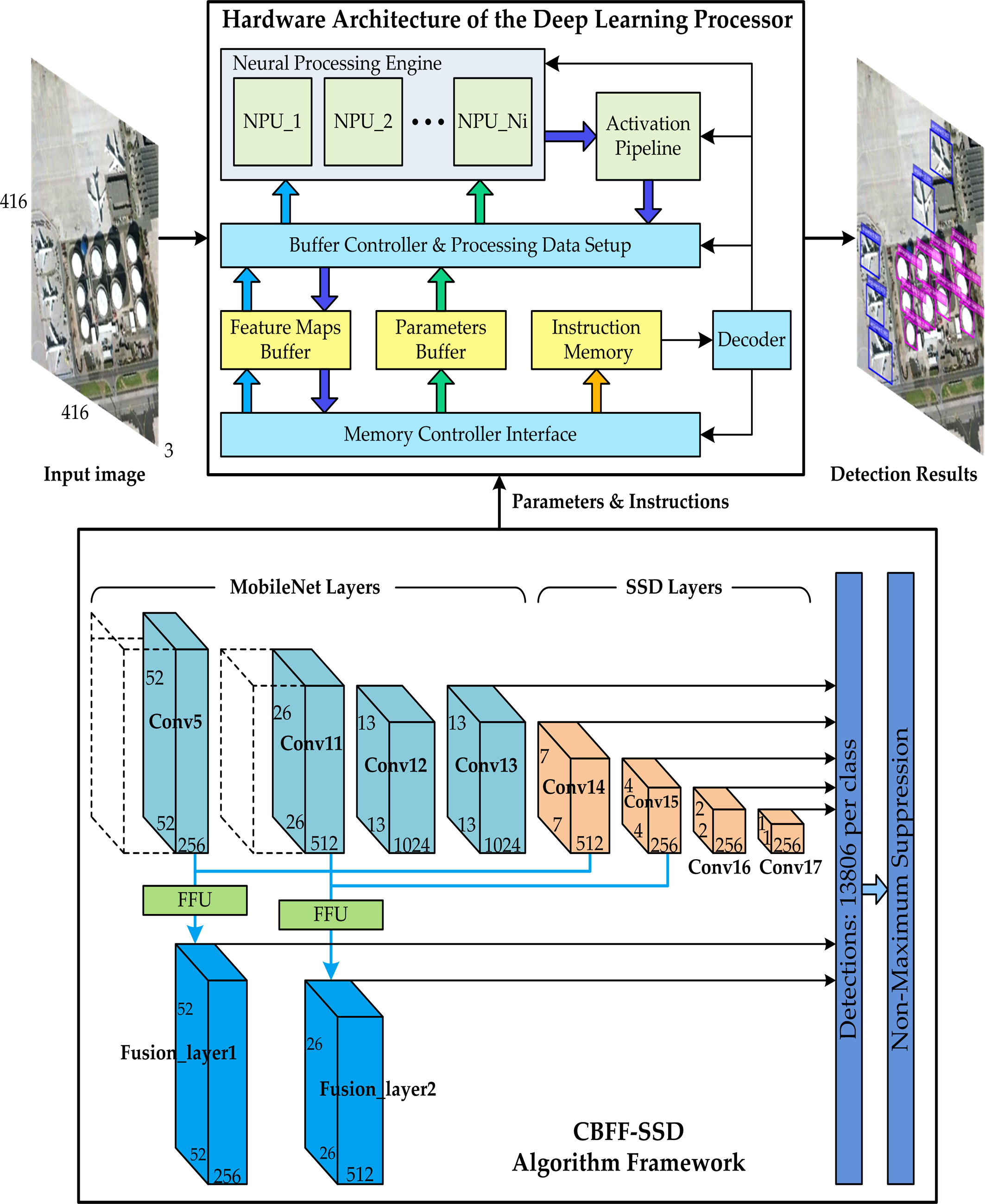
4. Hardware Architecture of Deep Learning Processor
In order to adapt to the high performance and low power consumption environment on the satellite or aircraft, we used the dedicated deep learning processor to replace the traditional CPUs or GPUs for object detection algorithm processing. Due to various considerations, the deep learning hardware architecture we designed only supports the calculation of the algorithm inference stage, and the training and the acquisition of parameters are realized by the offline mode.
Based on the characteristics of algorithmic hierarchical computing and the analysis and optimization of the calculation of each layer in deep learning algorithm in
Section 3, we designed the hardware architecture of deep learning processor shown in
Figure 3. Our deep learning processor consists of the following main components: memory controller interface, feature maps buffer, parameters buffer, instruction memory, decoder, buffer controller and processing data setup module, neural processing engine, and activation pipeline module.
The memory controller interface interacts with the outside system through the advanced extensible interface (AXI) bus. It stores the received image data, parameters, and instructions into the feature maps buffer, the parameters buffer, and instruction memory respectively, and returns the calculation result of the deep learning processor to the system. The feature maps buffer is used to store input and output feature maps. The parameters buffer is used to store the weight and bias parameters obtained by offline training. The instructions of deep learning processor are stored in the instruction memory. After the instruction is decoded, the control signals are respectively transmitted to the respective functional modules. The buffer controller and processing data setup module readout feature maps data and parameters, and then sends them to the neural processing engine after organization, and stores the calculated output feature maps data of the activation pipeline module into the feature maps buffer. The neural processing engine performs basic neuron operations such as multiplication, addition and comparison. The activation pipeline module is used to implement an approximate calculation of the nonlinear activation function.
4.1. Parallel Computing Architecture
In the image object detection application, the input and output feature maps are both three-dimensional. According to the characteristics of the feature map, we naturally thought of parallel computing for three different dimensions in calculation. However, in the current research, most designs were performed in parallel for a two-dimensional neuron of an output feature map until this one was finished and next one began [
35,
36,
37,
38,
39,
40,
41,
42,
43,
44]. Therefore, we designed multiple neural processing units (NPUs) in the neural processing engine to realize parallel computing of multiple output feature maps. The hardware architecture of neural processing engine we designed is shown in
Figure 4.
We designed N
i neural processing units (NPUs) in the neural processing engine, which can simultaneously calculate the N
i output feature maps. The buffer controller and processing data setup module provides neurons and synapses for each neural processing unit for calculation. It reads data from the feature maps buffer and parameters buffer and reorganizes it for distribution to the neural processing units. After the calculation is completed, the neural processing engine outputs to the activation pipeline module for processing, and then writes the results to the feature maps buffer-by-buffer controller. The neural processing unit (NPU) consists of P
x × P
y processing elements (PEs) arranged in 2-D format. As can be seen from the right part of
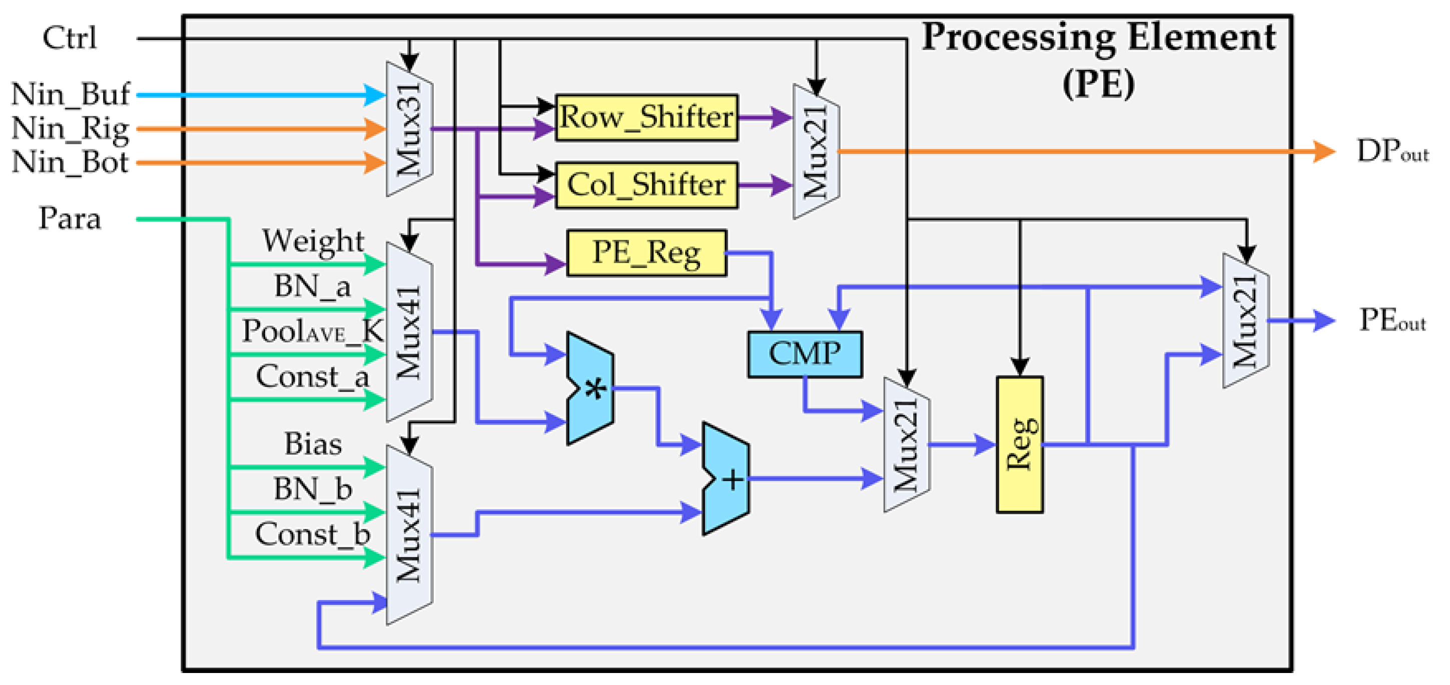
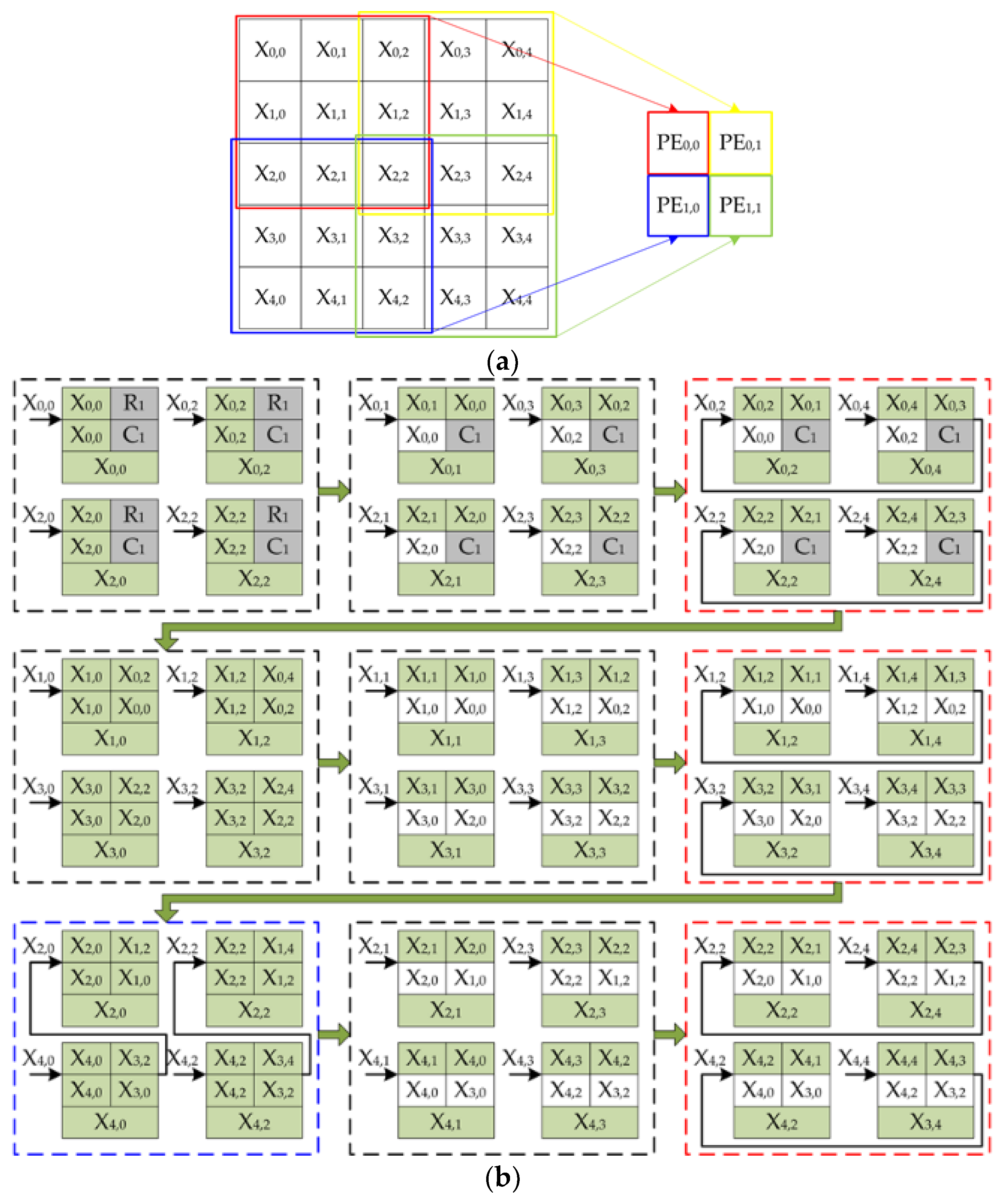
Figure 4, the neuron data calculated by the PEs could come not only from the buffer controller but also from right or bottom PEs. The data propagation between the PEs achieved data reuse, and reduced the bandwidth of reading the feature maps buffer.
The data propagation path and the computation path were designed in the PE structure shown in
Figure 5 to implement data reuse and neuron calculation functions respectively. The data propagation path was used for local transfer of neuron data between PEs, thereby realizing data reuse. Inspired by the calculation process of the sliding window during image convolutional operations, the input of this path included three ways of reading from the buffer controller and reading from the right or bottom PE. We set two sets of shifter registers in this path, which were row shift register (Row_Shifter) and column shift register (Col_Shifter). These registers were used to implement temporary storage and propagation of the reused neuron data. Based on the analysis of many current mainstream deep learning algorithms and the object detection algorithm proposed in
Section 2, the stride of convolutional operations generally did not exceed 2. Therefore, in each set of shift registers we set up two serially connected 16-bit registers to form a queue. The specific use of these two registers was detailed in the
Section 4.3 data sharing and reuse. The hardware structure of the computation path included a multiplexer, multiplier, adder, comparator, and register. The computation path mainly completed the calculation of the PE, which supported multiplication, addition and comparison operations, and implemented all the calculation of the algorithm layers except for activation function and Softmax. When the computation path worked, the neuron data came from the PE_Reg, and the parameters were selected according to the calculation of each layer. For example, weight and bias were used for the calculation of convolutional layer, and two pre-processed parameters BN_a and BN_b for the computation of the normalization layer.
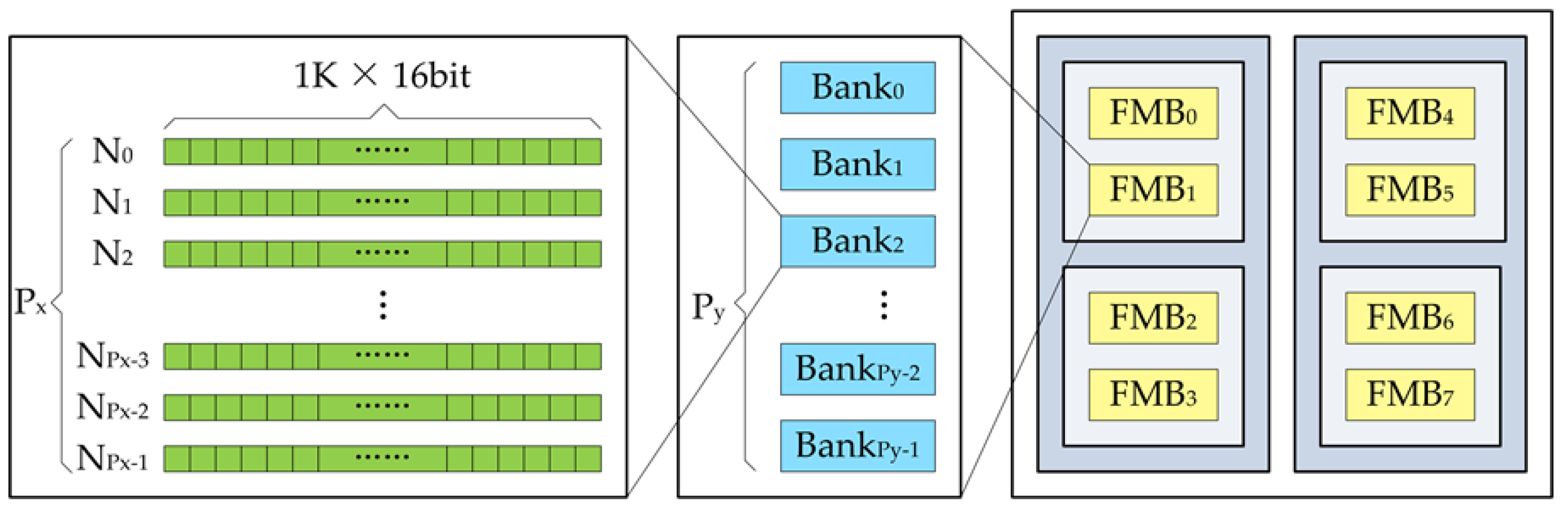
4.2. Hierarchical Storage Organization
The application of object detection in a remote sensing image is not only computation intensive, but also storage-intensive. Therefore, the efficient calculation of the neural processing engine is inseparable from the efficient organization and timely delivery of neuron data. The hierarchical storage organization structure as show in
Figure 6 was adopted to store the feature maps in our design.
We can see from the
Figure 6, the structure of the feature map buffer was related to the number of PEs in the NPU. We designed P
x independent 16-bit width memory in one bank, where P
x is the number of PEs in a row of the NPU. Designing with independent memory made it easy for us to address a single neuron. In the upward level of storage, we designed P
y banks, where P
y is the number of PEs in a column of the NPU. This design allowed us to not only address a single neuron, but also read P
x × P
y neurons in one clock period. In order to achieve greater memory bandwidth, we could also design the separate memory similar to the multi-port format of the register file. The feature map buffer was divided into eight blocks, each of which contained P
y banks. Each of the two memory blocks constituted a set of Ping-Pong memories for alternately storing input or output feature maps. When a set of memory (e.g., FMB
0 and FMB
1) is the input feature map buffer, another set (e.g., FMB
2 and FMB
3) is used to store the output feature map. The input and output characteristics of the buffer were alternately changed, and the current output feature map buffer was the input feature map buffer calculated by the next layer of the algorithm. The other half of the buffer was used as a temporary buffer to handle data interactions of large algorithm when the feature maps size was larger than the on-chip buffer capacity. At this time, the two halves of the buffer acted as Ping-Pong memory to achieve alternate storage of the feature maps.
In order to effectively read out neuron data and reorganize it, the buffer controller reads the feature map buffer in four ways:
Read Px × Py neurons from Py banks.
Read Px neurons from 1 bank.
Read Py neurons from Py banks with given stride.
Read a single neuron.
These four reading modes can complete the reading of the neuron data in each layer of the deep learning algorithm.
The parameters buffer mainly stores the weights and bias data of the convolutional layer and the preprocessing parameters of the normalization layer. Due to the parameter sharing feature in the convolutional network, the structure of the parameters buffer is slightly different from the feature map buffer. The parameters buffer contains two levels storage structure. We designed Ni independent memories in its first level storage for a bank, where Ni is the number of NPUs. The second level storage contains four independent banks, which form two sets of Ping-Pong memory. In order to adapt to the large-scale model, the two sets of buffer were alternately used for the storage of current parameters and the interaction of subsequent parameters. The parameters are sequentially stored in the first-level independent memory according to the dimensions of the output feature map. The instruction buffer was designed as a FIFO (first input first output) with a width of 128 bits and a depth of 2 k. The very long instruction word (VLIW) instructions are sequentially stored in it. Since the structure of the instruction buffer is simple, it will not be described more here.
4.3. Data Sharing and Reuse
In order to reduce the bandwidth of the read buffer and perform calculations efficiently, and to make full use of the weight sharing of the convolutional neural network, we took a lot of work in the design of the deep learning processor. Taking the convolutional operation with the largest amount of calculation in the object detection algorithm as an example, since the N
i NPUs share the input neurons, only the P
x × P
y neurons data are read out and broadcast to the N
i NPUs for calculation in the first cycle. At the same time, the weights are shared within the NPU, and only the N
i weights are read from the parameters buffer and sent to the corresponding NPU for calculation. In the subsequent cycles of convolutional operation, not only data sharing but also data reuse based on inter-PE neuron propagation was adopted. The specific process of data reuse based on inter-PE neuron propagation in the convolutional operation is show in
Figure 7 and
Figure 8.
We can see from
Figure 7 that when stride was equal to 1, neuron reuse used only one row register and one column register for 3 × 3 convolutional operations. The row and column shift registers in the PE could be configured by the control signal to write neuron data directly to the output stage registers while masking the first stage registers. When Stride was equal to 1, the data could be reused for all cycles of the convolutional operation except for the first cycle. Specifically, (K
x − 1) × K
y row propagations were performed, and (K
y − 1) column propagations were performed, where K
x and K
y was the kernel size.
Based on the analysis of many current mainstream deep learning algorithms and the object detection algorithm proposed in
Section 2, the stride of convolutional operations generally did not exceed 2. Therefore, in each set of shift registers in PE we set up to two serially connected 16-bit registers to form a queue. We can see from
Figure 8, for a convolutional operation with a stride equal to 2, only four 16-bit registers were needed to achieve data reuse, which saved hardware resources compared to the design of FIFO for six 16-bit storage cells in [
40]. When stride was equal to 2, taking 3 × 3 convolution as an example, data reuse could be performed in only four cycles. Fortunately, this situation was a small percentage of the calculation in the algorithm.
Data sharing and reuse were mainly applied to the convolutional layer, the normalized layer, and the fully connected layer. The remaining layers required a larger buffer read bandwidth because there was no overlapping of data.


