Article

Sub-Daily Temperature Heterogeneity in a Side Channel and the Influence on Habitat Suitability of Freshwater Fish

by
Frank P.L. Collas
1,2,3,*,
Wimala K. van Iersel
4,
Menno W. Straatsma
4,
Anthonie D. Buijse
5 and
Rob S.E.W. Leuven
2,3
1
Institute for Water and Wetland Research, Department of Animal Ecology and Physiology, Radboud University, P.O. Box 9010, 6500 GLNijmegen, The Netherlands
2
Institute for Water and Wetland Research, Department of Environmental Science, Radboud University, P.O. Box 9010, 6500 GL Nijmegen, The Netherlands
3
Netherlands Centre of Expertise on Exotic Species (NEC-E), P.O. Box 9010, 6500 GL Nijmegen, The Netherlands
4
Faculty of Geosciences, Department of Physical Geography, Utrecht University, P.O. Box 80115, 3508 TS Utrecht, The Netherlands
5
Department of Freshwater Ecology and Water Quality, Deltares, P.O. Box 85437, 3508 AL Utrecht, The Netherlands
*
Author to whom correspondence should be addressed.
Remote Sens. 2019, 11(20), 2367; https://doi.org/10.3390/rs11202367
Submission received: 13 August 2019 / Revised: 28 September 2019 / Accepted: 5 October 2019 / Published: 12 October 2019
(This article belongs to the Section Environmental Remote Sensing)

Abstract

:
Rising surface water temperatures in fluvial systems increasingly affect biodiversity negatively in riverine ecosystems, and a more frequent exceedance of thermal tolerance levels of species is expected to impoverish local species assemblages. Reliable prediction of the effect of increasing water temperature on habitat suitability requires detailed temperature measurements over time. We assessed (1) the accuracy of high-resolution images of water temperature of a side channel in a river floodplain acquired using a consumer-grade thermal camera mounted on an unmanned airborne vehicle (UAV), and (2) the associated habitat suitability for native and alien fish assemblages. Water surface temperatures were mapped four times throughout a hot summer day and calibrated with 24 in-situ temperature loggers in the water at 0.1 m below the surface using linear regression. The calibrated thermal imagery was used to calculate the potentially occurring fraction (POF) of freshwater fish using species sensitivity distributions. We found high temperatures (25–30 °C) in the side channel during mid-day resulting in reduced habitat suitability. The accuracy of water temperature estimates based on the RMSE was 0.53 °C over all flights (R2 = 0.94). Average daily POF was 0.51 and 0.64 for native and alien fish species in the side channel. The error of the POF estimates is 76% lower when water temperature is estimated with thermal UAV imagery compared to temperatures measured at an upstream gauging station. Accurately quantifying water temperature and the heterogeneity thereof is a critical step in adaptation of riverine ecosystems to climate change. Our results show that measurements of surface water temperature can be made accurately and easily using thermal imagery from UAVs allowing for an improved habitat management, but coincident collection of long wave radiation is needed for a more physically-based prediction of water temperature. Because of climate change, management of riverine ecosystems should consider thermal pollution control and facilitate cold water refugia and connectivity between waterbodies in floodplains and the cooler main channel for fish migration during extremely hot summer periods.

Graphical Abstract

1. Introduction

Water temperature is a key environmental factor directly and indirectly affecting survival of aquatic species such as macrophytes [1], macro-invertebrates [2] and fish [3,4]. Climate change will increase water temperatures of rivers on all continents [5], further increasing environmental stress in riverine ecosystems. When water becomes too warm, detrimental stress occurs in many species ultimately resulting in mortality [6,7,8]. In addition, increasing temperature facilitates the spread and establishment of alien species [9,10,11,12], which increases their competition success with native species and causes biotic homogenization. Alien fish species already dominate freshwater fish assemblages in many rivers of the world [13,14,15], urging the need to assess the effect of increasing water temperatures under a changing climate on native and alien fish species.
The thermal limits of freshwater fish species can be used to construct species sensitivity distributions (SSDs) [10,16,17]. These statistical distributions describe the variation of species sensitivity to an environmental factor [18]. Using SSDs, the relationship between the potentially occurring fraction (POF) of a species assemblage and the magnitude of an environmental pressure can be derived [17,19]. The POF represents the fraction of the maximum number of native and alien fish species that can potentially occur in water with based on the assessed environmental factor. SSDs allow predicting habitat suitability for the assessed species group based on single or multiple environmental factors [10,11,20]. The availability of field data that reflect the spatiotemporal variation of the temperature is vital for predicting thermal habitat suitability of native and alien fish using SSDs.
Water temperature of rivers shows a high spatiotemporal variability [21,22]. Spatial variation in temperatures results from inflow of tributaries [23] and groundwater, shading by riparian vegetation [23], water depth [24], amongst other factors. The high spatiotemporal variability of water temperature limits the usability of point measurements to accurately assess habitat suitability [10,25]. This can partly be solved by modelling, but a temperature model capturing high spatiotemporal details requires a thorough knowledge on complex processes of the water body, which is often lacking [26].
Remote sensing of water surface temperature allows documenting spatiotemporal patterns in riverine habitat suitability [27,28]. The radiant temperature is derived from the thermal infrared radiation (TIR) emitted by the water surface using Planck’s Law and the emissivity of water [29]. It is important to note that measurements of emitted TIR only represent the top 100 µm of the water column [27] and that the highly reflective water surface can disturb the thermal signal of the water by reflecting TIR from the sun directly into the sensor [30]. The reflection effect varies over time due to changes in solar angle and wind conditions. Previous studies have mapped water temperature of rivers and/or streams using airborne thermal imagery with an average error varying between 0.3 and 2.5 °C (Supporting information: Table S1). Aircrafts and helicopters have been used most often to carry the thermal sensors, but these are expensive to deploy, especially for small areas and repeated observations.
A potential method to measure spatiotemporal variation in water temperatures in small water systems (e.g., side channels of 10–30 m wide) are unmanned airborne vehicles (UAVs) [31]. Their availability increases and they are being deployed with a large variety of sensors, ranging from simple consumer-grade cameras [32] to hyperspectral [33], LiDAR [34] and thermal infrared sensors [35]. The latter may offer new opportunities to address the problem of spatial monitoring of water temperature. UAVs are easy to deploy compared to an aircraft or helicopter. They offer a high spatial resolution (<1 m), which depends on the flight elevation and sensor resolution. However, it remains unclear whether water temperature can be estimated by UAVs with sufficient accuracy for monitoring habitat suitability for freshwater fish.
This research aimed to predict thermal habitat suitability of a side channel in the littoral zone of rivers during hot summer conditions using thermal imagery. We define thermal imagery as the remotely sensed temperature measurements using a UAV. The research questions were: (1) How accurately can water temperature be measured using thermal imagery? (2) What is the spatiotemporal temperature variation during a hot day? (3) What is the added value of using thermal imagery to predict the habitat suitability for native and alien fish species compared to commonly used in-situ measurements or gauge data? (4) How does the temperature error in thermal images propagate to the estimation of habitat suitability?

2. Materials and Methods
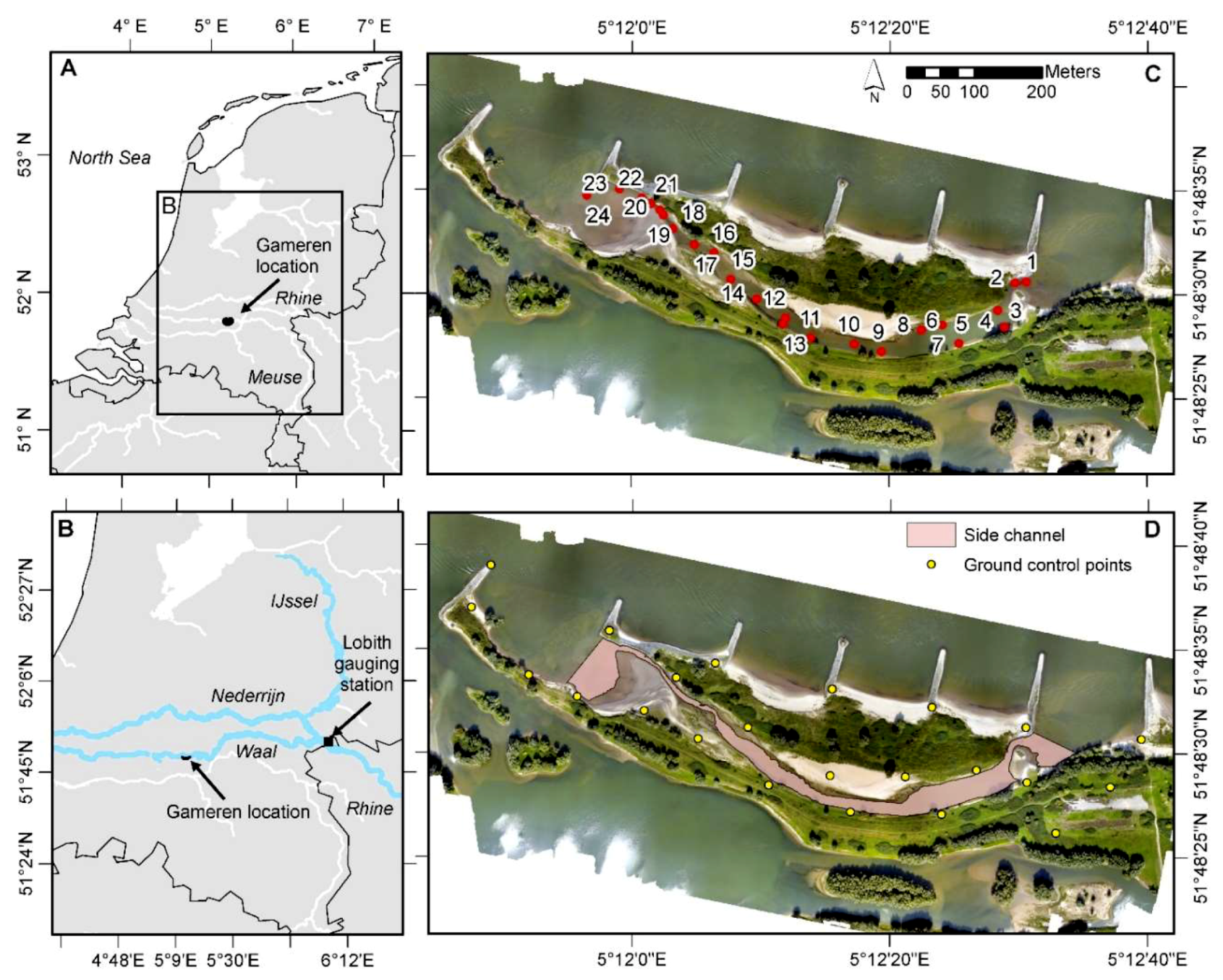
To map the temperature fields and the associated potentially occurring fraction (POF) for native and alien species, we collected the thermal imagery and field reference data, which were combined with species sensitivity distributions (SSDs) from the literature (Figure 1). Here, we explain the methodological steps in detail.

2.1. Study Area

The river Waal is the main distributary of the river Rhine in the Netherlands (Figure 2a,b). As part of the ecological restoration, three side channels were created between 1996 and 1999 near the village of Gameren: two flow year-round and one flows only during higher river discharges. Air temperature at a height of 1.5 m on 29 August 2017, varied between 12.5 and 29.6 °C, with a mean temperature of 21.6 °C. Wind speed during that day varied between 1.0 and 4.0 m.s−1 (www.knmi.nl). The water level at gauging station Lobith was 8.03 m and the discharge was 1362 m3.s−1 (www.waterinfo.rws.nl).
Water temperature measurements were performed at 24 locations in the northern side channel (Figure 2c). We chose the smallest side channel that has an open connection during low flow, because of the expected spatiotemporal variability in temperature due to: (1) variations in depth and (2) the propagation of ship-induced waves from the main channel from both the upstream and downstream end. Most locations were characterized by low flow conditions, but substantial bidirectional flow was found near the in- and outflow of the side channel (location 1, 19, 22, 23 and 24). During the measurement day, flow velocities were measured with peak values of 35 cm s−1 (SD = ± 10 cm s−1) using a propeller flow meter.

2.2. Thermal Iimagery

A ThermoMAP sensor mounted to a Sensefly Ebee UAV [36] was used to collect thermal imagery at four different moments during a day on 29 August 2017 (Table 1). The ThermoMAP sensor performs an automatic temperature calibration in-flight based on the sensor’s internal temperature and assumes an emissivity of 1 for the surveyed surface. Flight duration was approximately 15 min per flight and the entire study area was covered in a single flight. To improve georeferencing of the imagery, 23 ground control points (GCPs) were distributed along both banks of the side channel (Figure 2d) and were georeferenced with a Trimble dGPS, which had a horizontal and vertical accuracy of 0.015 and 0.02 m, respectively. The GCPs were vinyl disks with a 50 cm diameter covered with tinfoil with a low emissivity (5%) to guarantee their visibility on thermal imagery. A georeferencing error <0.1 m was obtained.

2.3. In-Situ Measurements

Time series of temperature measurements were performed by positioning waterproof loggers (Hobo Onset, accuracy 0.5 °C) 10 cm below the water surface at 24 locations distributed across the side channel (Figure 2c) covering variation in depth and flow velocity. At locations 6, 14, 16 and 24 the water depth was sufficiently deep to perform additional temperature measurements at a depth of 50 cm. The loggers measured water temperature with a frequency of 0.1 Hz and were geolocated with the Trimble dGPS.

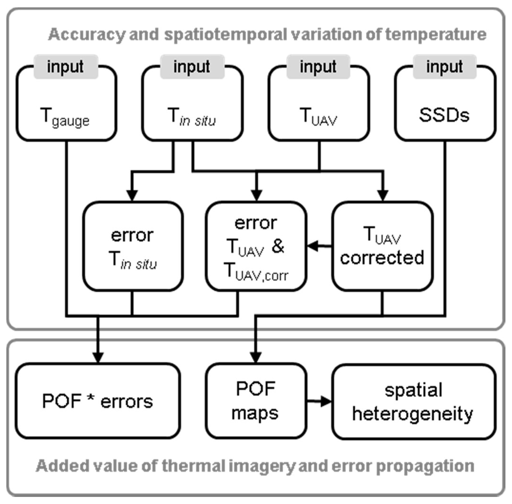
2.4. Pre-Processing and Accuracy Assessment

The ThermoMAP output image files were orthorectified with the SenseFly Postflight Terra software to create orthophotos. After initial matching based on the given geolocation of the images by the UAV-mounted GPS, the imagery was georeferenced manually with the GCPs. The temperature values as registered by the sensor were rescaled to temperatures in °C (TUAV). In-situ water temperatures at 10 cm depth (Tref.10) and 50 cm depth (Tref.50) were calculated as the median of each logger’s measurement over the 15-min duration of each flight (Table 1). TUAV values were extracted from the thermal imagery at the logger’s locations and used to calculate the mean absolute error (MAE). The MAE of the thermal imagery expresses the error in water temperature without calibration with field data. Subsequently, a linear regression was performed to establish empirical relationships between (1) Tref.10 and TUAV to determine the error in water temperature after calibration with field data and (2) Tref.10 and Tref.50 to estimate the relation between water temperatures at different water depths. Linear regression equations and root mean squared errors (RMSE) were calculated for each flight separately and for all flights combined. This RMSE expresses the residual error after calibration. No further correction for water emissivity was applied due to lack of data on incoming long wave radiation during the UAV flight.

2.5. Spatiotemporal Temperature Changes and Habitat Suitability

2.5.1. Water Temperature Variation

The overall regression equation between TUAV and Tref.10 was used to correct the TUAV orthophotos (TUAV,corr) using the R statistics package Raster [38,39]. The TUAV,corr maps where used to assess heterogeneity in water temperature in the side channel spatial subset (Figure 2d) by constructing boxplots of the temperatures of the pixels included in the subset.

2.5.2. Added Value of Using Thermal Imagery to Predict the Habitat Suitability

Two SSDs for water temperature sensitivity of native and alien fish species occurring in the river Rhine (Figure 3) were derived from data of Leuven et al. [10] based on the maximum temperature tolerance of 35 native fish species and 22 alien fish species that occur in the river Rhine. SSDs are constructed by fitting a normal distribution to known maximum temperatures of a local species assemblage, resulting in a maximum temperature SSD. The resulting SSD can then be used to derive the potentially occurring fraction (POF) of the assessed species assemblage based on measured or modelled temperatures. We derived separate POF values for native and alien fish species at specific water temperatures. A POF value of 0.5 for the native fish indicates that 50% of the species assemblage is tolerant of the ambient water temperature and is able to potentially occur if other habitat requirements are also met.
In this study, the TUAV,corr maps were used as temperature input for the SSDs thereby yielding a spatial POF map. We assessed the added value of thermal imagery by comparing habitat suitability using the thermal imagery (TUAV and TUAV,corr) and the habitat suitability estimated using gauge data or in-situ measurements. Gauge data are measured water temperatures of the main channel at the gauging station Lobith (Tgauge) 75 km upstream of the study area (Figure 2b). In-situ measurements were used to spatially model temperature using ordinary kriging [40].

2.5.3. Temperature Error Propagation

The error propagation provides insight into the sensitivity of the POF to errors in temperature measurements. We calculated the propagation of four temperature errors to investigate the effect of the temperature errors over the full range of the maximum temperature SSD on habitat suitability, assuming the temperature error is not dependent on the water temperature. The first three errors were the difference in temperature compared to the in-situ temperatures (Tref.10). The first error was the difference with Tgauge. The second error was the MAE, as this is the error without the correction of the thermal images with the in-situ temperatures (TUAV). The third error was the overall RMSE, as an indication of the error with the corrected thermal images (TUAV,corr). The fourth error was the overall RMSE of a leave-one-out-cross-validation (LOOCV) based on the ordinary kriging of the in-situ measurements. Each error was used to create an error band around the temperature for the entire range of the maximum temperature SSD. Subsequently, POF values were determined for each error corrected temperature and the maximum deviations in POF as a result of these errors were compared with each other.
To estimate the effect of the temperature error on the spatial POF, we also mapped the POF using the uncorrected TUAV (assuming Tref.10 = TUAV) and calculated the difference between POF maps obtained with TUAV,corr and TUAV. By mapping the differences, it became spatially explicit where the influence of the temperature error on the habitat suitability is largest.

3. Results

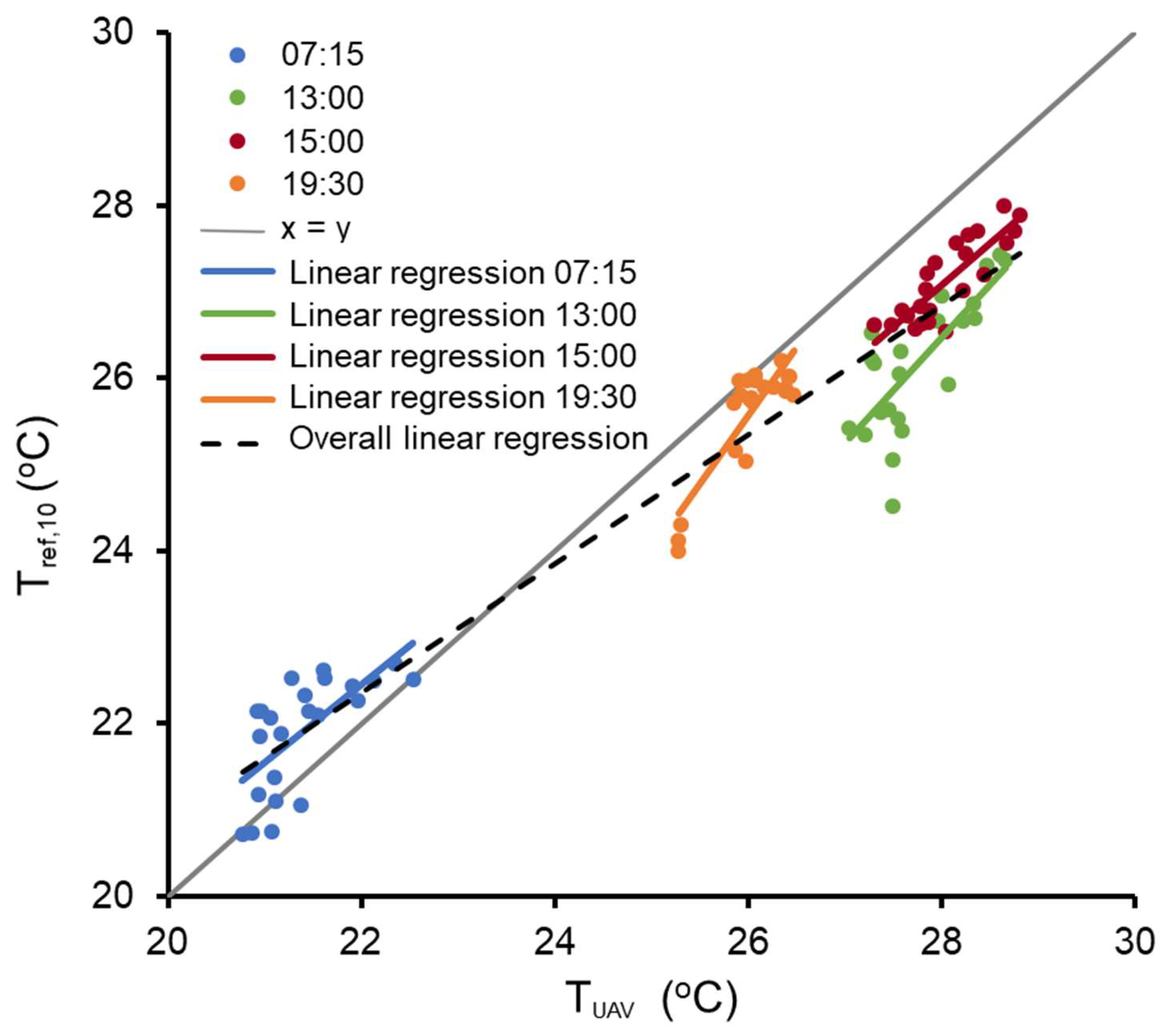
3.1. Thermal Imagery Accuracy Assessment

The mean absolute error (MAE) between TUAV and Tref.10 varied over the four flight campaigns between 0.58 and 1.58 °C (Table 2). The MAE over the four campaigns together was 0.81 °C. The largest errors of more than 3 times the SD (Table 2) were measured at 13:00 at locations 2, 4, 7, 8 and 13. Relatively large errors were also found at the inflow and outflow of the side channel at locations 1, 2, 19–22. The smallest errors were recorded during the 19:30 flight.
At 07:15, temperatures were mostly underestimated by TUAV in contrast with the other surveys, which showed an overestimation of Tref.10 (Figure 4). The regression equation of the 15:00 flight was closest to the y = x line, which is ideal when estimating temperature from thermal imagery. The morning and mid-day (13:00) flight performed worst regarding their regression functions with an R2 < 0.6. The regression between the TUAV and the Tref.10 based on data of all four surveys had a RMSE of 0.53 °C (Table 2). The LOOCV of the kriged in-situ measurements showed a lower average RMSE of 0.34 °C. A significant relationship was also found between the Tref.10 and Tref.50 measurements with a R2 value of 0.87 (Table 2). In addition, we have measured differences between Tref.10 and Tref.50 of 1.2 ± 0.2 °C during the 13:00 flight, while the differences were only 0.4 ± 0.5 °C during the other flights. This supports that the vertical gradient in temperature was highest during mid-day.

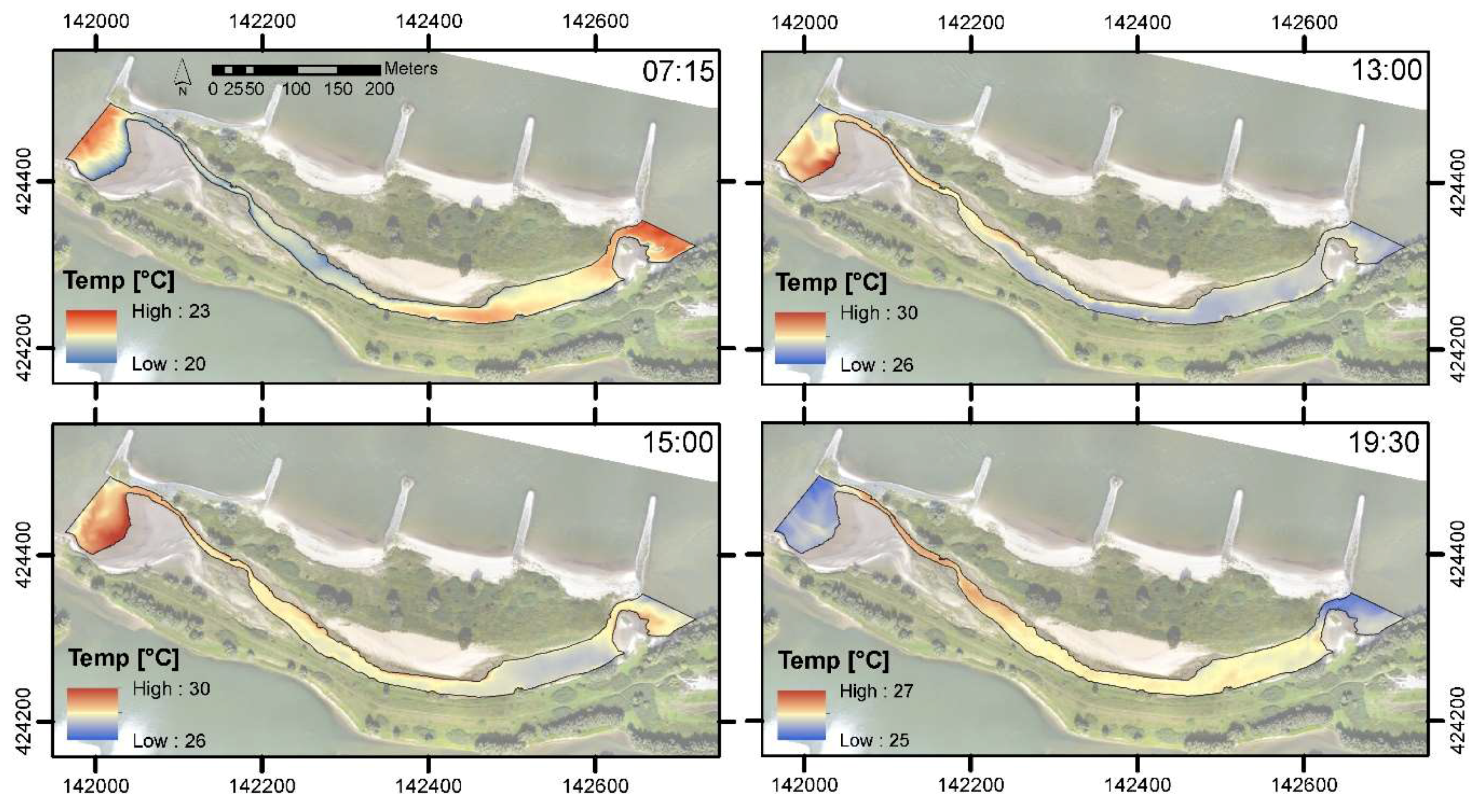
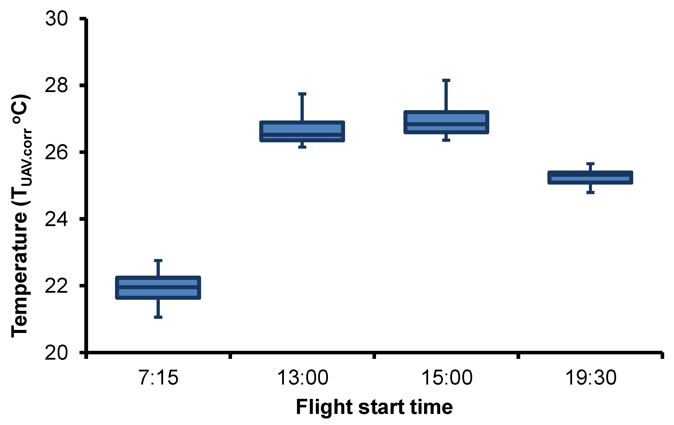
3.2. Spatiotemporal Variation of Temperature in the Side Channel

In general, the side channel was characterized by a higher water temperature during mid-day (13:00 and 15:00) than in the morning (07:15) (Figure 5; Figure 6). In the morning (07:15), the lowest temperatures were found in the shallow and narrow sections in the western part of the side channel and close to the banks (Figure 5). In the afternoon (13:00 and 15:00) the highest temperatures were found in these areas. In the evening (19:30), the temperatures remained highest between the narrow in- and outflow compared to the outer sections, which were more under influence of the main channel. Temperatures decreased during the mid-day to lower temperatures at 19:30. The observed average value of TUAV,cor increased over the course of the day: 21.95 ± 0.43°C at 07:15; 26.66 ± 0.43 °C at 13:00; 26.94 ± 0.46 °C at 15:00 and 25.25 ± 0.22 °C at 19:30.

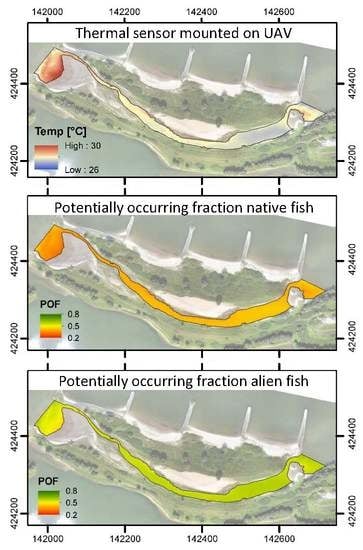
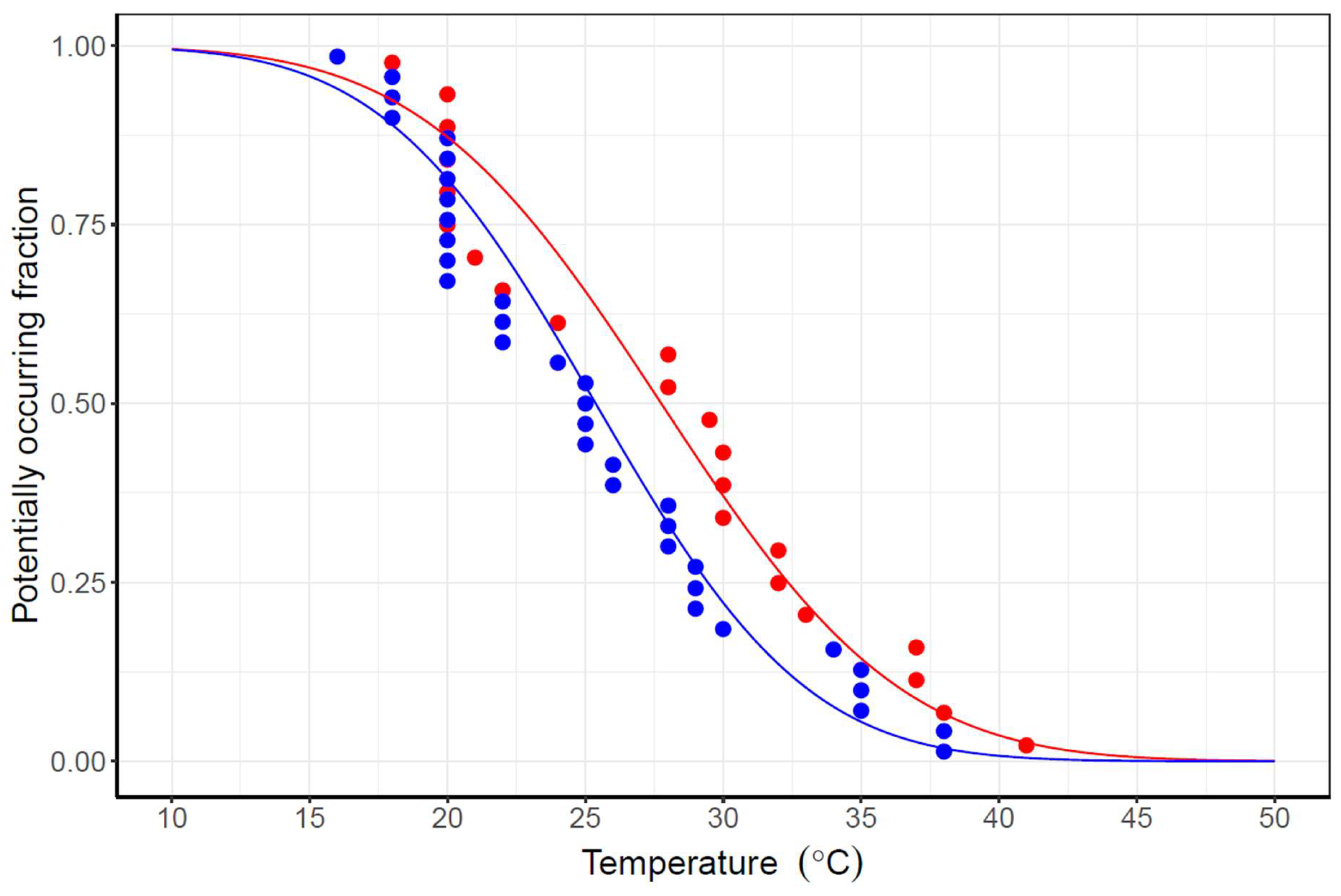
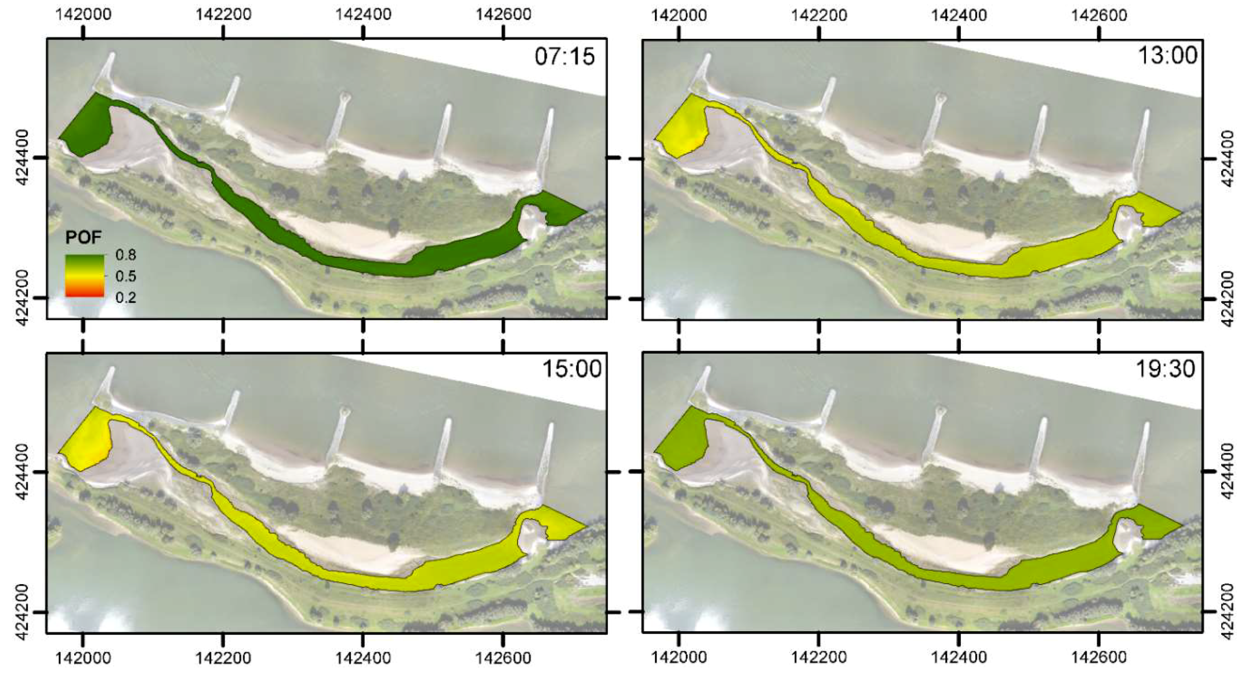
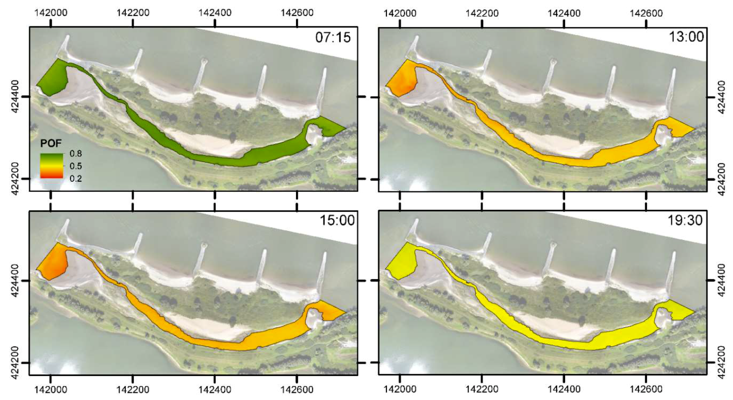
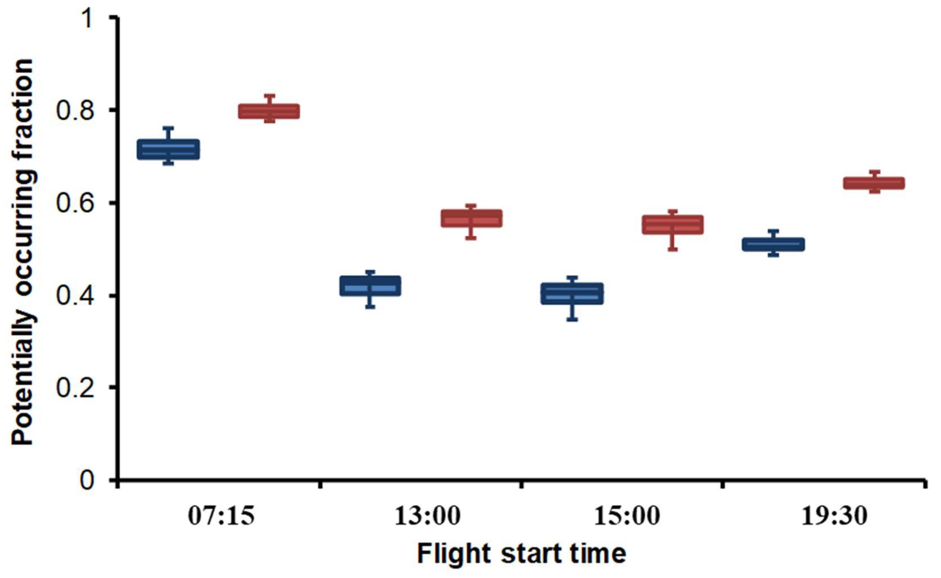
3.3. Habitat Suitability

The observed spatiotemporal patterns in water temperature were reflected in the calculated POF for alien (Figure 7) and native (Figure 8) fish species in the side channel. The higher POF values were obtained during the morning. Lowest POF values were derived at mid-day after which POF values increased at 19:30. Average daily POF value of alien fish species was 0.64 whereas for native fish species this value was lower (0.51) (Figure 9). This implies that throughout the day a larger number of native fish species (on average 13%) was limited by high water temperature than alien species. Additional analysis of the POF at 50 cm depth showed higher potential during mid-day at these increased depths (Supporting information: Figures S1 and S2) compared with shallow habitats (Figure 7; Figure 8), because of lower temperatures at larger depth. The average daily POFs using Tgauge (ranging between 22 and 23 °C, Supporting information: Figure S3) revealed higher POFs compared to the side channel for native fish species (0.51 vs. 0.65–0.71) as well as alien species (0.64 vs. 0.75–0.80).

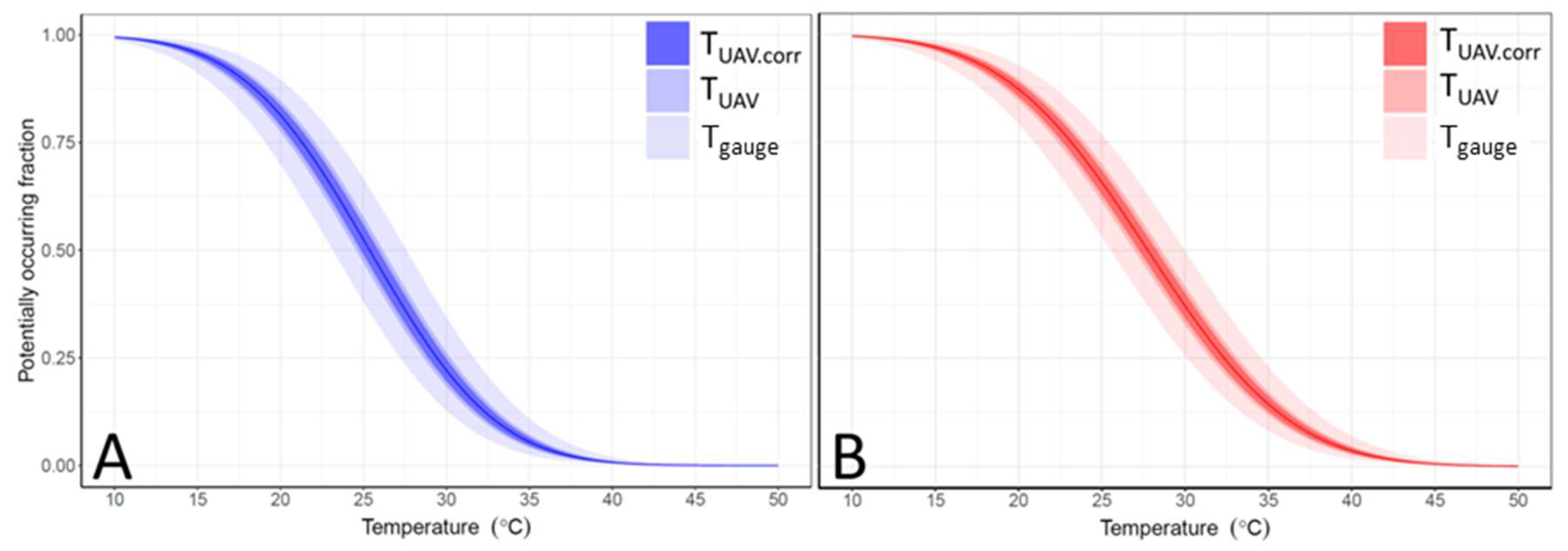
3.4. Temperature Error Propagation to Habitat Suitability

Errors in water temperature affect the POF estimates differently throughout the range of the maximum temperature SSD (Figure 10). A main observation is that the sensitivity of the POF estimation tapers off towards the extreme temperatures (10 °C and 37 °C). The error results in a range of possible POF values for a single estimated temperature, for example, at 25 °C the POF varies between 0.38 and 0.67 when estimated from a gauge temperature measurement.
The effect of the error also varies for the different methods of the temperature measurements. The Tgauge error was 2.2 °C and resulted in the largest uncertainty on the POF of native and alien fish, with maximum uncertainty of −0.146 to 0.146. The uncorrected TUAV error (MAE of 0.81°C) improved the POF estimations to an uncertainty of maximum ±0.054 for native and alien fish, which is a decrease in error of 0.093 (63% of the original error of 0.146 with Tgauge). Using the TUAV,corr error (RMSE of 0.53 °C), the POF uncertainty was minimized to a maximum of ± 0.035 for both native and alien fish species (Figure 10), which shows a decrease in uncertainty of 0.111 (76%) compared to using Tgauge and 0.018 (35%) compared to using TUAV. Errors were largest at shallow sections with high water level fluctuations. The LOOCV error based on the in-situ measurements was the smallest (0.34 °C) and, hence, resulted in the smallest uncertainty of POF estimations, e.g., −0.022 to 0.022. The propagation of the LOOCV error is not shown in Figure 10 for the sake of readability of the figure.

4. Discussion

4.1. Accuracy of Thermal Imagery to Estimate Water Temperature

The UAV thermal images of our field study yielded water temperature measurements with a MAE of 0.81 °C and at a high spatial (0.25 m) and temporal (four times per a single day) resolution. An extensive literature research of eight previous studies using thermal sensors in riverine environments (Table S1) reported an error ranging between −7 and 2.6 °C. Torgersen et al. [41] and Fullerton et al. [42] found lower errors, which can be explained by the more advanced sensors they used. However, these sensors are approximately ten times heavier than the ThermoMAP, and need to be deployed on a helicopter or aircraft, significantly decreasing their flexibility and increasing the costs for monitoring. Water temperature errors less than 1 °C were found in studies with (1) a sensor resolution smaller than the width of the rivers or lakes, to prevent a mixed signal with the non-aquatic temperatures of the banks, (2) reference water temperature measurements in the surface water layer (top 10 cm) and not near bottom of a water body, and (3) a relatively large sensor wave length range within the thermal infrared (8–12 µm) ([41,42,43]; Supporting information: Table S1). These aspects should be considered for future monitoring campaigns.
The accuracies of the thermal images varied over the day and between locations. Time variation in accuracy is generally attributed to changes in sun angle [30], wind-driven turbulence and mixing as a result of water depth fluctuation [44]. The highest absolute errors were found during the 13:00 flight. A potential explanation for this high error might be that at midday, solar irradiation and thermal stratification of the water are high as found by Handcock et al. [42]. This results in larger differences between the remotely sensed temperature of the water surface and the reference measurements below the surface. Hence, caution should be taken when using thermal imagery collected during mid-day. The difference in water temperature and air temperature is an additional factor given the difference in sampling depth over the columns. At 07:15 the surface could be cooled by the air, whereas later in the day the air temperature exceeds the water temperature. This can explain the overestimation of TUAV after 07:15. Furthermore, temperature estimates at locations that were shaded by trees during a flight were less accurate than those at non-shaded locations. Near the in- and outflow, accuracy was most likely reduced due to fast water level fluctuations due to passing ships and the resulting rough water surface, changing the water emissivity [45]. We have performed an empirical correction for emissivity and incoming long-wave radiation with the in-situ measurements. This was acceptable given the limited expected overestimation less than 0.5 °C resulting from the high emissivity of water (>0.95) [46]. For a more physically based approach it is necessary to correct for the actual water emissivity and incoming long-wave radiation. However, the latter is not a standard meteorological parameter and has a high spatial variation. The best approach would be to also measure incoming long-wave radiation with a sensor mounted on the UAV during the flight, comparable to a hand-held spectrometer. The accuracy of the regression functions to estimate water surface temperature is also affected by spatial autocorrelation of the reference measurements. Variograms of the reference measurements showed ranges of 142 m to 250 m for the different surveys, indicating the effective sample size for the regression is smaller due to the dependence of samples close to each other. Future studies can improve their error estimation by taking the effect of autocorrelation in their reference samples into account.

4.2. Spatiotemporal Variation of Water Temperature and Habitat Suitability

Multitemporal maps of water temperatures in the side channel show a natural pattern of warming mid-day and subsequent cooling in the evening. The magnitude of this sub-daily variation in water temperature likely differs between the measured side channel and nearby groyne fields. A groyne field is the riverine area between groynes which are hydraulic engineering structures that has been constructed across river banks in order to increase water flow in the main channel. Scour holes at the end of these groynes combined with the continuous mixing of water layers by intensive navigation changes the sub-daily variation in water temperature [47,48,49]. To confirm this, in-situ measurements over the day in the groyne fields are needed.
Spatial variation of water temperature can be subdivided in horizontal and vertical variation. The horizontal spatial variation in the side channel shows that the shallow sections are relatively cool in the morning and relatively warm during mid-day. The vertical variation strongly depends on vertical mixing of the water column. The strong correlation between the Tref.10 and the Tref.50 in the side channel shows that remotely sensed thermal imagery may also be used to estimate water temperatures at depths greater than 50 cm. However, this will require ground truthing using loggers at various water depths.
During mid-day the POFs of native and alien fish species decreased as temperature rose, whereas in the evening the POFs increased again. Fish avoid exposure to high temperature by diel migration to colder habitats such as deeper habitats in the side channel, the main channel or groyne fields which act as thermal refugia [50,51,52].
In the main channel and groyne fields, fish are exposed to other stressors that are virtually absent in side channels, such as ship-induced changes in flow velocity and water levels [53]. Although these stressors are not necessarily as detrimental as high water temperatures, they may have a negative effect on the energy expenditure of fish [54,55]. Further research should focus on elucidating the extent and the cost-benefit ratio of diel migrations of freshwater fish species occurring in the river Rhine due to high temperatures as investigated by Armstrong et al. [56] for juvenile Coho Salmon. During colder seasons the elevated temperatures in side channels during the day might be beneficial as growth of larval and juvenile stages of many fish species increases with higher temperatures [57].
Alien fish species have on average higher temperature tolerances compared to native fish species [10]. As water temperatures were very high at mid-day, the side channel has a limited habitat function for native fishes, whereas in the evening the side channel can serve as a refugium, showing the need of spatiotemporal temperature measurements. This need is further supported by the error in POF estimates with Tgauge compared to TUAV. The Tgauge-based POF for native and alien fish species were overestimated by 0.093 compared to the TUAV-based POF. This overestimation translates into the absence of three native and two alien species based on a species richness of 35 native and 22 alien species in the river Rhine [10].

4.3. Added Value of Thermal Imagery to Estimate Water Temperature and Habitat Suitability

The use of UAV-based thermal imagery decreased the uncertainty in POF estimates compared to estimates using existing data from the gauging station by 63%. This improvement was even larger when the thermal imagery was calibrated with in-situ measurements (76%). These results indicate the added value of thermal imagery to model temperature-based habitat suitability of freshwater fishes, similar as in studies by Vatland et al. [22] and Dzara et al. [25]. Even without in-situ calibration, uncertainty in POF estimates is greatly reduced by using temperatures measured with thermal imagery. Even though the prediction error was lowest with the kriged water temperature using the dense network of in-situ measurements (0.35 °C), the thermal imagery is more efficient to collect and results in highly accurate temperature measurements. A UAV flight took 15 min compared to multiple hours to set up the dense network of in-situ sensors. Moreover, waterbodies with a high spatial variability in temperature, i.e., due to seepage, have a high risk of underestimating this heterogeneity with in-situ sensors [22,25]. Hence, UAVs offer a fast and flexible solution to estimate water temperature at microhabitat scale. Thermal imagery can be an efficient approach for evaluating the effects of various types of ecological restoration measures on temperature regimes of the littoral zone of rivers. For instance, along the rivers Rhine and Meuse numerous restoration measures have been taken to improve the ecological status of these rivers [58,59,60,61]. These measures often aim to (re)create spawning and nursery areas and improve habitat suitability of rheophilous fish species. Our results show that during summer periods, high water temperatures in side channels negatively affect a substantial number of native fish species. During these periods, connectivity of the side channel with the main channel is vital as it allows diel migration, enabling fish to reach habitat with suitable conditions.
To meet river management at reach scale (~100 km), Vatland et al. [22], Dzara et al. [25] and Torgersen et al. [41] performed their surveys on a much larger extent than the current study (~1 km). They studied temperature heterogeneity relevant for fish using and migrating through these large extents. As a result of this large extent, TIR images were collected in a single flight from airplanes, which have a proven high accuracy but are not easily repeated for monitoring purposes. The relatively small extent of restoration measures such as restored side channels makes them especially suitable to be studied with UAVs and our results show that these platforms provide thermal imagery with enough accuracy to monitor water temperature and its variation. The need for frequent monitoring related to the innovative status of these measures is an additional argument for the use of UAVs, because of their low cost and flexibility to deploy.
A trade-off exists between the application of thermal imagery using UAVs and the spatial and temporal scale assessed. Our study shows that within a 15-min window, water surface temperature could be measured for an area with dimensions of roughly 1000 m by 500 m. With the ongoing improvement of UAV flight time combined with a cost reduction, applicability of UAV-based thermal imagery will increase. Detailed spatial and temporal water temperature measurements allow pinpointing management decisions at the spatial scales at which species actually occur, the microhabitat. Thus, the approach enables a fast assessment of habitat suitability quickly showing bottlenecks and identifying locations where improvements are necessary. From a scientific perspective, the spatial and temporal detail combined with species monitoring increases our fundamental understanding of habitat utilization and species preferences.

4.4. Recommendations for Side Channels as Floodplain Restoration Measure

Restoration measures should aim at optimizing abiotic conditions for native fish species as alien fish species can have severe ecological impacts [62]. It might therefore be valuable to improve the thermal potential for native fishes by increasing discharge of side channels, thereby increasing water circulation through them and reducing water temperatures [63]. In addition, deeper and shaded sections can serve as cold water refugia at mid-day during warm summers [23,49,64].
To maintain habitat suitability of a side channel during low water levels, when connectivity with the main channel becomes insufficient, colder refuge areas need to be available within the side channel. Measures to preserve habitat locations of sufficiently low water temperature comprise increasing discharge through side channels, and creating deeper and shaded sections that serve as refugia during extremely hot summer periods. Such adaptations are needed because these periods are expected to occur more frequently in near future [65]. In addition, restoration measures in areas with a sufficient slope in the water table can be designed in such a way that colder seepage water enters the restored water body from surrounding soil. Our approach can be used to periodically evaluate the temperature regimes of riverine ecosystems from a habitat-suitability perspective thereby giving input to decision making on adaptive management strategies such as a consistent connectivity with the main channel and cyclic rejuvenation of side channels [66].

5. Conclusions

UAV-borne thermal imagery can be used to measure water temperature in a river side channel with high accuracy (RMSE = 0.53 °C). The side channel was characterized by spatiotemporal variation in water temperature, with the shallow sections showing relatively low temperatures in the morning and relatively high temperatures in the afternoon. During a hot day, high temperatures (25–30 °C) in the side channel resulted in reduced habitat suitability especially affecting native species. These high water temperatures stress the need to facilitate diel migration or to provide cold-water refugia. Furthermore, the use of thermal imagery decreased uncertainty in habitat-suitability estimations compared to gauging-station measurements and provided additional information on spatial patterns of temperature and habitat suitability. In this study, we established empirical relationships between UAV-borne thermal imagery and field reference data. For future studies we recommend measuring incoming long-wave radiation with a sensor mounted on the UAV to allow a more physically based prediction of the water surface temperature. UAVs offer fast and flexible water-temperature estimation at microhabitat scale, compared to time-consuming in-situ measurements.

Supplementary Materials

The following are available online at https://www.mdpi.com/2072-4292/11/20/2367/s1, Figure S1: Measured water temperatures in the river Rhine at gauging station Lobith during 2017, Figure S2: The potentially occurring fraction (POF) of alien species in the river Waal near Gameren derived from remotely sensed water temperatures at 50 cm depth during a hot summer day, Figure S3: The potentially occurring fraction (POF) of native species in the river Waal near Gameren derived from remotely sensed water temperatures at 50 cm depth during a hot summer day, Table S1: Literature overview of thermal remote sensing of surface water temperature.

Author Contributions

Conceptualization, F.P.L.C., W.K.v.I., and M.W.S.; data curation, F.P.L.C. and W.K.v.I.; Formal analysis, F.P.L.C. and W.K.v.I.; Methodology, F.P.L.C., W.K.v.I., M.W.S. and R.S.E.W.L.; Supervision, M.W.S., A.D.B. and R.S.E.W.L.; Funding acquisition, R.S.E.W.L.; Validation, F.P.L.C. and W.K.v.I.; Visualization, F.P.L.C. and W.K.v.I., Writing—original draft, F.P.L.C. and W.K.v.I.; Writing—review & editing, F.P.L.C., W.K.v.I., M.W.S., A.D.B. and R.S.E.W.L.

Funding

This research is part of the research programme RiverCare, supported by the Dutch Technology Foundation TTW (formerly STW), which is part of the Netherlands Organization for Scientific Research (NWO), and which is partly funded by the Ministry of Economic Affairs under grant number P12–14 (Perspective Programme).

Acknowledgments

The authors would like to thank M.G. Kleinhans for his input during the initial idea development and Rijkswaterstaat for providing the bathymetry of the study site. H. Middelkoop, E.A. Addink and M.M. Schoor are thanked for their valuable proof reading of the manuscript. We also thank three anonymous reviewers for their suggestions to improve our manuscript.

Conflicts of Interest

The authors declare no conflict of interest.

References

  1. Bornette, G.; Puijalon, S. Response of aquatic plants to abiotic factors: A review. Aquat. Sci. 2011, 73, 1–14. [Google Scholar] [CrossRef]
  2. Burgmer, T.; Hillebrand, H.; Pfenninger, M. Effects of climate-drive temperature changes on the diversity of freshwater macroinvertebrates. Oecologia 2007, 151, 93–103. [Google Scholar] [CrossRef] [PubMed]
  3. Lehtonen, H. Potential effects of global warming on northern European freshwater fish and fisheries. Fish. Manag. Ecol. 1996, 3, 59–71. [Google Scholar] [CrossRef]
  4. Jackson, D.A.; Peres-Neto, P.R.; Olden, J.D. What controls who is where in freshwater fish communities - the role of biotic, abiotic, and spatial factors. Can. J. Fish. Aquat. Sci. 2001, 58, 157–170. [Google Scholar] [CrossRef]
  5. Van Vliet, M.T.H.; Franssen, W.H.P.; Yearsley, J.R.; Ludwig, F.; Haddeland, I.; Lettenmaier, D.P.; Kabat, P. Global river discharge and water temperature under climate change. Global Environ. Chang. 2013, 23, 450–464. [Google Scholar] [CrossRef]
  6. Souchon, Y.; Tissot, L. Synthesis of the thermal tolerances of the common freshwater fish species in large Western Europe rivers. Knowl. Manag. Aquat. Ec. 2012, 405, 03. [Google Scholar] [CrossRef]
  7. Koopman, K.R.; Collas, F.P.L.; Van der Velde, G.; Verberk, W.C.E.P. Oxygen can limit heat tolerance in freshwater gastropods: Differences between gill and lung breathers. Hydrobiologia 2016, 763, 301–312. [Google Scholar] [CrossRef]
  8. Verberk, W.C.E.P.; Leuven, R.S.E.W.; Van der Velde, G.; Gabel, F. Thermal limits in native and alien freshwater peracarid Crustacea: The role of habitat use and oxygen limitation. Funct. Ecol. 2018, 32, 926–936. [Google Scholar] [CrossRef] [Green Version]
  9. Rahel, F.J.; Olden, J.D. Assessing the effects of climate change on aquatic invasive species. Conserv. Biol. 2008, 22, 521–533. [Google Scholar] [CrossRef]
  10. Leuven, R.S.E.W.; Hendriks, A.J.; Huijbregts, M.A.J.; Lenders, H.J.R.; Matthews, J.; Van der Velde, G. Differences in sensitivity of native and exotic fish species to changes in river temperature. Curr. Zool. 2011, 57, 852–862. [Google Scholar] [CrossRef] [Green Version]
  11. Verbrugge, L.N.H.; Schipper, A.M.; Huijbregts, M.A.J.; Van der Velde, G.; Leuven, R.S.E.W. Sensitivity of native and non-native mollusc species to changing river water temperature and salinity. Biol. Invasions 2012, 14, 1187–1199. [Google Scholar] [CrossRef]
  12. Collas, F.P.L.; Buijse, A.D.; Hendriks, A.J.; Van der Velde, G.; Leuven, R.S.E.W. Sensitivity of European freshwater bivalve species to climate related environmental factors. Ecosphere 2018, 9, e02184. [Google Scholar] [CrossRef]
  13. Rahel, F.J. Homogenization of fish faunas across the United States. Science 2000, 288, 854–856. [Google Scholar] [CrossRef] [PubMed]
  14. Leprieur, F.; Beauchard, O.; Blanchet, S.; Oberdorff, T.; Brosse, S. Fish invasions in the world’s river systems: When natural processes are blurred by human activities. PLoS Biol. 2008, 6, 404–410. [Google Scholar] [CrossRef]
  15. Leuven, R.S.E.W.; Van der Velde, G.; Baijens, I.; Snijders, J.; Van der Zwart, C.; Lenders, H.J.R.; Bij de Vaate, A. The river Rhine: A global highway for dispersal of aquatic invasive species. Biol. Invasions 2009, 11, 1989–2008. [Google Scholar] [CrossRef]
  16. De Vries, P.; Tamis, J.E.; Murk, A.J.; Smit, M.G.D. Development and application of a species sensitivity distribution for temperature-induced mortality in the aquatic environment. Environ. Toxicol. Chem. 2009, 27, 2591–2598. [Google Scholar] [CrossRef] [PubMed]
  17. Del Signore, A.; Hendriks, A.J.; Lenders, H.J.R.; Leuven, R.S.E.W.; Breure, A.M. Development and application of the SSD approach in scientific case studies for Ecological Risk Assessment. Environ. Toxicol. Chem. 2016, 35, 2149–2161. [Google Scholar] [CrossRef]
  18. Posthuma, L.; Suter II, G.W.; Traas, T.P. Species Sensitivity Distributions in Ecotoxicology; Lewis Publishers: Boca Raton, FL, USA, 2002. [Google Scholar]
  19. Koopman, K.R.; Collas, F.P.L.; Breure, A.M.; Lenders, H.J.R.; Van der Velde, G.; Leuven, R.S.E.W. Predicting effects of ship-induced changes in flow velocity on native and alien molluscs in the littoral zone of lowland rivers. Aquat. Invasions 2018, 13, 481–490. [Google Scholar] [CrossRef]
  20. Collas, F.P.L.; Koopman, K.R.; Hendriks, A.J.; Van der Velde, G.; Verbrugge, L.N.H.; Leuven, R.S.E.W. Effects of desiccation on native and non-native molluscs in rivers. Freshw. Biol. 2014, 59, 41–55. [Google Scholar] [CrossRef]
  21. Caissie, D. The thermal regime of rivers: A review. Freshw. Biol. 2006, 51, 1389–1406. [Google Scholar] [CrossRef]
  22. Vatland, S.J.; Gresswell, R.E.; Poole, G.C. Quantifying stream thermal regimes at multiple scales: Combining thermal infrared imagery and stationary stream temperature data in a novel modelling framework. Water Resour. Res. 2014, 51, 31–46. [Google Scholar] [CrossRef]
  23. Ebersole, J.L.; Liss, W.J.; Frissell, C.A. Cold water patches in warm streams: Physicochemical characteristics and the influence of shading. J. Am. Water Resour. Assoc. 2003, 39, 355–368. [Google Scholar] [CrossRef]
  24. Matthews, K.R.; Berg, N.H.; Azuma, D.L.; Lambert, T.R. Cool water formation and trout habitat use in a deep pool in the Sierra Nevada, California. Trans. Am. Fish. Soc. 1994, 123, 549–564. [Google Scholar] [CrossRef]
  25. Dzara, J.R.; Neilson, B.T.; Null, S.E. Quantifying thermal refugia connectivity by combining temperature modeling, distributed temperature sensing, and thermal infrared imaging. Hydrol. Earth Syst. Sci. 2019, 23, 2965–2982. [Google Scholar] [CrossRef] [Green Version]
  26. Boyd, M.; Kasper, B. Analytical Methods for Dynamic Open Channel Heat and Mass Transfer; Technical report; Department of Environmental Quality: Portland, OR, USA, 2017.
  27. Handcock, R.N.; Torgersen, C.E.; Cherkauer, K.A.; Gillespie, A.R.; Tockner, K.; Faux, R.N.; Tan, J. Thermal infrared remote sensing of water temperature in riverine landscapes. In Fluvial Remote Sensing for Science and Management; John Wiley & Sons: New York, NY, USA, 2012; pp. 85–113. [Google Scholar]
  28. Turner, D.; Lucieer, A.; Malenovský, Z.; King, D.H.; Robinson, S.A. Spatial co-registration of ultra-high resolution visible, multispectral and thermal images acquired with a micro-UAV over Antarctic moss beds. Remote Sens. 2014, 6, 4003–4024. [Google Scholar] [CrossRef]
  29. Norman, J.M.; Becker, F. Terminology in thermal infrared remote sensing of natural surfaces. Int. J. Remote Sens. 1995, 12, 159–173. [Google Scholar] [CrossRef]
  30. Anderson, J.M.; Wilson, S.B. The physical basis of current infrared remote-sensing techniques and the interpretation of data from aerial surveys. Int. J. Remote Sens. 1984, 5, 1–18. [Google Scholar] [CrossRef]
  31. DeBell, L.; Anderson, K.; Brazier, R.E.; King, N.; Jones, L. Water resource management at catchment scales using lightweight UAVs: Current capabilities and future perspectives. J. Unmanned Veh. Syst. 2015, 4, 7–30. [Google Scholar] [CrossRef]
  32. Van Iersel, W.; Straatsma, M.; Middelkoop, H.; Addink, E. Multitemporal Classification of River Floodplain Vegetation Using Time Series of UAV Images. Remote Sens. 2018, 10, 1144. [Google Scholar] [CrossRef]
  33. Näsi, R.; Honkavaara, E.; Lyytikäinen-Saarenmaa, P.; Blomqvist, M.; Litkey, P.; Hakala, T.; Holopainen, M. Using UAV-based photogrammetry and hyperspectral imaging for mapping bark beetle damage at tree-level. Remote Sens. 2015, 7, 15467–15493. [Google Scholar] [CrossRef]
  34. Khan, S.; Aragão, L.; Iriarte, J. A UAV–lidar system to map Amazonian rainforest and its ancient landscape transformations. Int. J. Remote Sens. 2017, 38, 2313–2330. [Google Scholar] [CrossRef]
  35. Nishar, A.; Richards, S.; Breen, D.; Robertson, J.; Breen, B. Thermal infrared imaging of geothermal environments by UAV (unmanned aerial vehicle). J. Unmanned Veh. Syst. 2016, 4, 136–145. [Google Scholar] [CrossRef]
  36. SenseFly Drones for Professionals, Mapping & Photogrammetry, Flight Planning & Control Software. Available online: https://www.sensefly.com/home.html (accessed on 12 December 2017).
  37. SenseFly Our Camera Payloads & Accessories. Available online: https://www.sensefly.com/drones/accessories.html (accessed on 25 January 2018).
  38. R Core Team R: A Language and Environment for Statistical Computing. R Foundation for Statistical Computing: Vienna, Austria, 2015. Available online: https://www.R-project.org/ (accessed on 25 January 2018).
  39. Hijmans, R.J.; Van Etten, J.; Cheng, J.; Mattiuzzi, M.; Sumner, M.; Greenberg, J.A.; Perpinan Lamigueiro, O.; Bevan, A.; Racine, E.B.; Shortridge, A.; et al. Package Raster - Geographic Data Analysis and Modelling. Available online: https://cran.r-project.org/web/packages/raster/raster.pdf (accessed on 23 January 2018).
  40. Cressie, N. Statistics for Spatial Data; John Wiley: New York, NY, USA, 1993. [Google Scholar]
  41. Torgersen, C.E.; Faux, R.N.; McIntosh, B.A.; Poage, N.J.; Norton, D.J. Airborne thermal remote sensing for water temperature assessment in rivers and streams. Remote Sens. Environ. 2001, 76, 386–398. [Google Scholar] [CrossRef]
  42. Fullerton, A.H.; Torgersen, C.E.; Lawler, J.J.; Faux, R.N.; Steel, E.A.; Beechie, T.J.; Leibowitz, S.G. Rethinking the longitudinal stream temperature paradigm: Region-wide comparison of thermal infrared imagery reveals unexpected complexity of river temperatures. Hydrol. Process. 2015, 29, 4719–4737. [Google Scholar] [CrossRef]
  43. Dugdale, S.J.; Bergeron, N.E.; St-Hilaire, A. Spatial distribution of thermal refuges analysed in relation to riverscape hydromorphology using airborne thermal infrared imagery. Remote Sens. Environ. 2015, 160, 43–55. [Google Scholar] [CrossRef]
  44. Handcock, R.N.; Gillespie, A.R.; Cherkauer, K.A.; Kay, J.E.; Burges, S.J.; Kampf, S.K. Accuracy and uncertainty of thermal-infrared remote sensing of stream temperatures at multiple spatial scales. Remote Sens. Environ. 2006, 100, 427–440. [Google Scholar] [CrossRef]
  45. Henderson, B.G.; Theiler, J.; Villeneuve, P. The polarized emissivity of a wind-roughened sea surface: A Monte Carlo model. Remote Sens. Environ. 2003, 88, 453–467. [Google Scholar] [CrossRef]
  46. Prakash, P. Thermal remote sensing: Concepts, issues and applications. Int. Arch. Photogramm. Remote Sens. Spat. Inf. Sci. 2000, 33, 239–243. [Google Scholar]
  47. Yousef, Y.A.; McLellon, W.M.; Zebuth, H.H. Changes in phosphorus concentrations due to mixing by motorboats in shallow lakes. Water Res. 1980, 14, 841–852. [Google Scholar] [CrossRef]
  48. Becker, A.; Kirchesch, V.; Baumert, H.Z.; Fischer, H.; Schöl, A. Modelling the effects of thermal stratification on the oxygen budget of an impounded river. River Res. Appl. 2010, 26, 572–588. [Google Scholar] [CrossRef]
  49. Engel, F.; Fischer, H. Effect of thermal stratification on phytoplankton and nutrient dynamics in a regulated river (Saar, Germany). River Res. Appl. 2017, 33, 135–146. [Google Scholar] [CrossRef]
  50. Clough, S.; Ladle, M. Diel migration and site fidelity in a stream-dwelling cyprinid, Leuciscus leuciscus. J. Fish. Biol. 1997, 50, 1117–1119. [Google Scholar] [CrossRef]
  51. Borcherding, J.; Bauerfeld, M.; Hintzen, D.; Neumann, D. Lateral migrations of fishes between floodplain lakes and their drainage channels at the Lower Rhine: Diel and seasonal aspects. J. Fish. Biol. 2002, 61, 1154–1170. [Google Scholar] [CrossRef]
  52. Hohausová, E.; Copp, G.H.; Jankovský, P. Movement of fish between a river and its backwater: Diel activity and relation to environmental gradients. Ecol. Freshw. Fish. 2003, 12, 107–117. [Google Scholar] [CrossRef]
  53. Collas, F.P.L.; Buijse, A.D.; Van den Heuvel, L.; Van Kessel, N.; Schoor, M.M.; Eerden, H.; Leuven, R.S.E.W. Longitudinal training dams mitigate effects of shipping on environmental conditions and fish density in the littoral zones of the river Rhine. Sci. Total Environ. 2018b, 619–620, 1183–1193. [Google Scholar] [CrossRef]
  54. Schiemer, F.; Keckeis, H.; Kamler, E. The early life history stages of riverine fish: Ecophysiological and environmental bottlenecks. Comp. Biochem. Phys. A 2003, 133, 439–449. [Google Scholar] [CrossRef]
  55. Trinci, G.; Harvey, G.L.; Henshaw, A.J.; Bertoldi, W.; Hölker, F. Life in turbulent flow interactions between hydrodynamics and aquatic organisms in rivers. WIREs Water 2017, 4, e1213. [Google Scholar] [CrossRef]
  56. Armstrong, J.B.; Schindler, D.E.; Ruff, C.P.; Brooks, G.T.; Bentley, K.E.; Torgersen, C.E. Diel horizontal migration in streams: Juvenile fish exploit spatial heterogeneity in thermal and trophic resources. Ecology 2013, 94, 2066–2075. [Google Scholar] [CrossRef]
  57. Nunn, A.D.; Cowx, I.G.; Frear, P.A.; Harvey, J.P. Is water temperature an adequate predictor of recruitment success in cyprinid fish populations in lowland rivers? Freshw. Biol. 2003, 48, 579–588. [Google Scholar] [CrossRef]
  58. Nienhuis, P.H.; Buijse, A.D.; Leuven, R.S.E.W.; Smits, A.J.M.; De Nooij, R.J.W.; Samborska, E.M. Ecological rehabilitation of the lowland basin of the river Rhine (NW Europe). Hydrobiologia 2002, 478, 53–72. [Google Scholar] [CrossRef]
  59. Van Stokkom, H.T.C.; Smits, A.J.M.; Leuven, R.S.E.W. Flood defense in the Netherlands: A new era, a new approach. Water Int. 2005, 30, 76–87. [Google Scholar] [CrossRef]
  60. Rijke, J.; Van Herk, S.; Zevenbergen, C.; Ashley, R. Room for the River: Delivering integrated river basin management in the Netherlands. Int. J. River Basin Manag. 2012, 10, 369–382. [Google Scholar] [CrossRef]
  61. Straatsma, M.W.; Bloecker, A.M.; Lenders, H.J.R.; Leuven, R.S.E.W.; Kleinhans, M.G. Biodiversity recovery following delta-wide measures for flood risk reduction. Sci. Adv. 2017, 3, e1602762. [Google Scholar] [CrossRef]
  62. Cucherousset, J.; Olden, J.D. Ecological Impacts of Non-native Freshwater Fishes. Fisheries 2011, 36, 215–230. [Google Scholar] [CrossRef]
  63. Sinokrot, B.A.; Gulliver, J.S. In-stream flow impact on river water temperatures. J. Hydraul. Res. 2000, 38, 339–349. [Google Scholar] [CrossRef]
  64. Kurylyk, B.L.; MacQuarrie, K.T.B.; Li, T. Preserving, augmenting, and creating cold-water thermal refugia in rivers: Concepts derived from research on the Miramichi River, New Brunswick (Canada). Ecohydrology 2015, 8, 1095–1108. [Google Scholar] [CrossRef]
  65. Christidis, N.; Jones, G.S.; Stott, P.A. Dramatically increasing chance of extremely hot summers since the 2003 European heatwave. Nat. Clim. Chang. 2015, 5, 46–50. [Google Scholar] [CrossRef]
  66. Baptist, M.J.; Penning, W.E.; Duel, H.; Smits, A.J.M.; Geerling, G.W.; Van der Lee, G.E.M.; Van Alphen, J.S.L. Assessment of the effects of cyclic floodplain rejuvenation on flood levels and biodiversity along the Rhine River. River Res. Appl. 2004, 20, 285–297. [Google Scholar] [CrossRef]
Figure 1. Flowchart to determine the accuracy of thermal imagery, calculate habitat suitability and to quantify the effect of the error in temperature on the POF estimations (T: temperature; UAV: unmanned airborne vehicle; SSD: species sensitivity distribution, POF: potentially occurring fraction).
Remotesensing 11 02367 g001
Figure 2. (a) Location of the study area in the Netherlands, (b) river Rhine tributaries in blue, with study area along the river Waal, (c) Aerial photo of the northern side channel and groyne fields with in-situ water temperature locations (red dots), (d) Side channel subsection of study area used for assessment of heterogeneity in water temperature.
Remotesensing 11 02367 g002
Figure 3. Species sensitivity distribution of maximum water temperature for native (blue; n = 35; μ = 25.4 °C; σ = 6.1 °C) and alien (red; n = 22; μ = 27.8 °C; σ = 7.0 °C) fish species occurring in the river Rhine (Data: Leuven et al. [10]). At 25 °C only 53% and 66% of the native and alien species pool can occur based on their thermal maxima, respectively.
Remotesensing 11 02367 g003
Figure 4. Regression of water temperature acquired using thermal imagery (TUAV) and the in-situ reference measurements (Tref.10).
Remotesensing 11 02367 g004
Figure 5. Temperature maps of the side channel in the floodplain of the river derived from uncorrected thermal imagery (°C, TUAV) during the morning (07:15), mid-day (13:00 and 15:00) and evening (19:30). Note the different color scales across the individual maps.
Remotesensing 11 02367 g005
Figure 6. Box plot of the corrected water temperatures (TUAV.corr) in the studied side channel. The centerline shows the median, the boxes indicate the 25% and 75% percentile and the whiskers depict the 2.5% and 97.5% percentile.
Remotesensing 11 02367 g006
Figure 7. The potentially occurring fraction (POF) of alien species in the northern side channel along the river Waal near Gameren derived from remotely sensed water temperatures during a hot summer day.
Remotesensing 11 02367 g007
Figure 8. The potentially occurring fraction (POF) of alien species in the northern side channel along the river Waal near Gameren derived from remotely sensed water temperatures during a hot summer day.
Remotesensing 11 02367 g008
Figure 9. The potentially occurring fraction (POF) of native (blue) and alien (red) fish species due to water temperatures during a summer day in the side channel. The centerline shows the median, the boxes indicate the 25% and 75% percentile and the whiskers indicate the 2.5% and 97.5% percentiles.
Remotesensing 11 02367 g009
Figure 10. Uncertainty in potentially occurring fraction (POF) due to propagation of temperature errors for (a) native species and (b) alien species. Temperature errors are the mean difference between the in-situ measured temperatures (TRef.10) compared to (1) the corrected thermal images (TUAV,corr; light shade), (2) the thermal images collected using an UAV (TUAV; medium shade) and (3) the measured temperature at the gauging station of Lobith (Tgauge; dark shade).
Remotesensing 11 02367 g010
Table 1. Characteristics of unmanned airborne vehicle (UAV) flights and sensor.
UAV Flights
Flight duration15 min
Flying altitude130 m
Flight start times07:15, 13:00, 15:00, 19:30
ThermoMAP sensor [37]
Ground resolution25 cm × 25 cm
Radiometric sensitivity7–15 µm
Max. response at10 µm
Temperature resolution0.1 °C
Temperature range−40 to +160 °C
Temperature calibrationAutomatic, in-flight
Output formatTIFF images
Weight of sensor~ 134 g
Table 2. Descriptive statistics of Tref.10 and the TUAV and the regression between the two during four UAV flights and for all flights combined. The last row shows the regression equation between Tref.10 and Tref.50, including its R2 and the overall UAV and LOOCV based RMSE of Tref.50.
Flight
Time
Average
Tref.10 (°C)
MAE (SD) +
(°C)
Regression Equation R2UAV RMSE †
(°C)
LOOCV RMSE ‡
(°C)
07:1521.900.58 (0.40)Tref.10 = 0.9025 TUAV + 2.58800.450.490.38
13:0026.191.58 (0.52)Tref.10 = 1.2218 TUAV + 7.73720.570.730.51
15:0027.130.92 (0.26)Tref.10 = 0.9595 TUAV + 0.21360.710.360.29
19:3025.610.42 (0.37)Tref.10 = 1.5732 TUAV – 14.3310.740.490.21
Overall24.940.81 (0.60)Tref.10 = 0.7469 TUAV + 5.93010.930.530.34
Tref.50 Tref.50 = 0.8085 Tref.10 + 4.24480.871.310.46
+ MAE: mean absolute error ± SD: standard deviation. † UAV RMSE: root mean squared error of the regression between TUAV and Tref.10 ‡ LOOCV RMSE: root mean squared error of leave-one-out-cross-validation analysis of in-situ measurements.

