Letter

Forest Connectivity, Host Assemblage Characteristics of Local and Neighboring Counties, and Temperature Jointly Shape the Spatial Expansion of Lyme Disease in United States

1
College of Life Sciences, Nanjing Normal University, Nanjing 210046, China
2
Resource Ecology Group, Wageningen University, 6708PB Wageningen, The Netherlands
*
Author to whom correspondence should be addressed.
Remote Sens. 2019, 11(20), 2354; https://doi.org/10.3390/rs11202354
Submission received: 2 August 2019 / Revised: 30 September 2019 / Accepted: 10 October 2019 / Published: 11 October 2019
(This article belongs to the Special Issue Remote Sensing for Public Health)

Abstract

:
Understanding risk factors for the spread of infectious diseases over time and across the landscape is critical for managing disease risk. While habitat connectivity and characteristics of local and neighboring animal (i.e., host) assemblages are known to influence the spread of diseases, the interactions among these factors remain poorly understood. In this study, we conducted a county-level analysis to test the effects of forest connectivity, together with the suitability of local assemblage (measured by the similarity of local host assemblage with neighboring assemblages) and the infection intensity of neighboring counties on the spatial expansion of Lyme disease in the United States. Our results suggested that both the similarity of local host assemblage and the infection intensity of neighboring counties were positively correlated with the probability of disease spread. Moreover, we found that increasing forest connectivity could facilitate the positive effect of neighbor infection intensity. In contrast, the effect size of the host assemblage similarity decreased with increasing connectivity, suggesting that host assemblage similarity was less effective in well-connected habitats. Our results thus indicate that habitat connectivity can indirectly influence disease spread by mediating the effects of other risk factors.

1. Introduction

Understanding the spatial expansion of infectious disease is important in predicting the new geographic areas that would have disease presence and is of importance in disease management [1]. The spreading rate of disease is not the same over different directions in space, which indicates the variation in spatial suitability for both host and vector [2]. This raises a question of what factor influences the nonrandom spread of disease over space.
In general, landscape structure can potentially affect the range expansion of disease due to its important role in determining host–pathogen interactions [3]. For example, it has been considered that habitat connectivity is able to considerably influence the process of disease spread via its effect on the dispersal and distributions of hosts and vectors [2,4,5] and host community compositions [6,7]. An increase in connectivity generally relates to an increase in the disease incidence or severity due to increased host movements and contact rates between host populations [8]. When studying the spread of plague epizootics in Colorado, Stapp and co-workers [9] found that increasing landscape connectivity promoted plague outbreaks in prairie dog colonies. However, high connectivity may sometimes reduce disease risk by increasing host diversity, which can exert a dilution effect [7], or by generating large epidemics that deplete susceptible individuals [10]. Thus, the role of habitat connectivity in disease spread still needs more investigations in the context of increasing habitat fragmentation worldwide.
Based on land cover data, we here investigated the effect of forest connectivity on the spread of Lyme disease in the United States. Lyme disease, caused by Borrelia burgdorferi and transmitted by Ixodes ticks [11], is recognized as an important emerging infectious disease [12]. Lyme disease in the United States undergoes rapid range expansions from its primary foci in the Upper Midwest and Northeast [13]. However, the rate of expansion varied within and among states. For example, some parts of states (i.e., counties) are rapidly invaded, whereas others remain disease-free for years [14]. Not only the distribution of Lyme disease, but also that of tick vector are expanding [15,16]. For example, Ixodes scapularis has moved northward along the eastern shores of Lake Michigan [16] and has also spread across the state from west to east in Wisconsin [17]. The large geographic range of Lyme disease and I. scapularis combined with the nonrandom spatial patterns in colonization raise important questions about the mechanisms driving expansion of this emerging infectious disease.
The dispersal and establishment of I. scapularis in new areas partly depend on the possibilities of dispersal of the tick hosts (carrying ticks) which rely on both host movements and landscape characteristics [14]. The former relates to the inherent capacities of host species to move (i.e., some species can more easily move over larger distances than others); the latter relates to parameters that help (e.g., corridors) or hinder (e.g., barriers) these movements. Because the dispersal probability of species that host I. scapularis partly drives the spread of Lyme disease [18,19], we predicted a positive relationship between forest connectivity and the probability of transition from disease-free to infected.
Besides landscape structure, the nonrandom expansion of disease via hosts or vectors can also be explained by characteristics of both the local and the neighboring host assemblages (e.g., all host species in a particular habitat/area), such as the suitability of local host assemblage (in disease-free areas) and the intensities of infected neighbors [20]. Due to host specificity of pathogens or vectors [21], the suitability of local disease-free assemblage could be partly explained by its similarity with neighboring infected (and infectious) assemblages. Greater ecological similarity can translate to less resistance of local disease-free assemblage to pathogen invasion, thus indicates high suitability to disease spread [20]. In addition, the infection intensity of infected neighbors might be positively related to the probability of disease spread. This is because high intensities of infected neighbors indicate high prevalence rates of the Lyme pathogen in ticks and hosts, which would enhance the chances that infected host or ticks invade to the disease-free county. In this study, we also explored the effects of these two factors on Lyme disease spread. We predict a positive relationship between the similarity of host assemblage in local disease-free area with neighboring infected areas and the probability that the disease-free area will become infected. We also predict that the infection intensity of neighboring infected areas relates positively to the probability of transition from disease-free to infected.
In addition, it is likely that the three factors described above (suitability of the assemblage in a disease-free area, the infection intensity of neighboring infected area, and the connectivity between disease-free and infected areas) also interact. For example, the effect of the intensity of infection in an area where the disease is present may depend on the connectivity level between disease-free and infected areas, so interactions between these factors are also expected to influence the geographical expansion of infectious disease. However, these interactions between connectivity and host assemblages similarity or infection intensity have rarely been studied. Therefore, in addition to the effects of these three factors, we also explicitly examined the importance of their two-way interactions to the transition in disease status (from disease-free to infected). Our results suggested that forest connectivity can indirectly influence disease spread by mediating the effects of assemblage suitability and neighbor infection intensity.

2. Materials and Methods

2.1. Lyme Disease Data

We first obtained the annual number of human Lyme disease cases in each county in the United States during 2000–2016 from the Centers for Disease Control and Prevention (CDC, Figure 1). We then limited our dataset to only those counties with established or reported I. scapularis populations, according to [11]. As we aim to identify factors related to a county’s transition of Lyme disease status, we targeted, per year, only those disease-free counties that shared a border with at least one infected county (at least one case was reported) in the same year. We then determined, also on an annual basis, whether a disease-free county remained disease-free or became infected in the next year. This binary classification served as the dependent variable in our analyses.

2.2. Explanatory Variables

Remote sensing (RS) has been recognized as an important tool for studying the ecology and epidemiology of infectious diseases [22]. It is often used to identify environmental (including habitat-related) and climatic risk factors, especially at regional level [23,24]. Using the National Land Cover Database (https://www.usgs.gov/centers/eros/science/national-land-cover-database) in United States Geological Survey, we calculated forest habitat connectivity. This parameter was calculated as the minimum percentage of forest over 1 km wide buffer zones on both sides of a shared border between two counties. For each county, forest connectivity was weighted by the length of shared borders (1):
Forest   connectivity = i = 1 n minimum   forest i l i i = 1 n l i
where n is the number of infected neighbors that shared borders with disease-free county; li = length of shared borders between focal disease-free county and the ith infected county.
Moreover, as Ixodes ticks are highly susceptible to desiccation, dry springs and summers may reduce the abundance of nymphal ticks in subsequent seasons [25,26,27]. Therefore, we extracted several climatic variables from the WorldClim database, version 2.0 [28], including Bio01 (mean annual temperature), Bio05 (maximum temperature of warmest month), Bio10 (mean temperature of warmest quarter), Bio12 (annual precipitation), Bio13 (precipitation of wettest month), Bio16 (precipitation of wettest quarter), and Bio18 (precipitation of warmest quarter). These variables were evaluated for possible inclusion as covariates in the model (Table 1). Habitat connectivity and climatic variables were calculated in ArcGIS (Version 10.5)
Similarity of local host assemblage for disease-free counties with neighboring infected counties (hereafter local assemblage similarity) was measured as β diversity using the Jaccard similarity index [29], based on the list of mammal host species of Ixodes scapularis from [11] which contains 39 mammal species. The distributions of these host species were obtained from the IUCN (International Union for Conservation of Nature) [30]. Similar to forest connectivity, host assemblage similarity, calculated in R 3.5.0 with vegan package [31], was weighted by the length of shared borders:
Local   assemblage   similarity = i = 1 n Jaccard   similarity i l i i = 1 n l i ,
The intensities of disease in infected neighboring counties (hereafter neighbor infection intensity) were calculated based on the numbers of reported Lyme disease cases and were weighted using the following formula:
Neighbor   infection   intensity = i = 1 n number   of   reported   disease   cases i P i i = 1 n P i ,
where Pi is the length of shared border between a disease-free focal county and the ith infected neighbor divided by the total border length of the focal disease-free county, thus, an infected neighboring county with a larger percentage of shared border was given greater weight.

2.3. Statistical Analyses

To explore the factors related to the probability of Lyme infection at the county level (i.e., the transition from disease-free to infected), we constructed Generalized Linear Mixed Models (GLMMs) with a binary response. State and year were included as random factors. Local assemblage similarity, neighbor infection intensity, forest connectivity, their two-way interactions, and climatic variables were included as fixed factors. We also included human population size of focal counties as an offset.
With GLMMs, we first performed univariate analyses to identify the potential risk factors. Variables with a p-value of less than 0.05 were identified as potential risk factors and were used to construct multiple regression models. Before constructing multiple models, we checked for multicollinearity by examining the correlation coefficients (r) between predictor variables. For those highly correlated (r > 0.7), only the variable with the smaller p-value was used to construct multiple regression models [32]. We performed backward selection to build a multiple model with only main effects, and then the interaction terms were included into the model. Main terms were maintained in the model if they were included in a significant interaction term. Before fitting models, all predictors were scaled. We reported the ROC (receiver operating characteristic) curve and AUC (Area under ROC curve) value to estimate the performance of the final model. All analyses were conducted using R 3.5.0 with lme4 package.

3. Results

For each year from 2000 to 2015, about 484 ± 65 counties were disease-free, and about 25% of these disease-free counties got infected in the next year (Table 2).
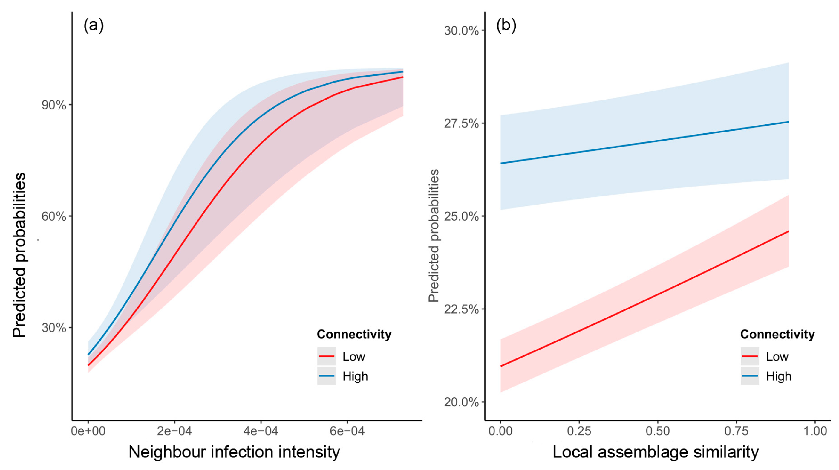
Based on the results of univariate analyses (Table S1) and the correlations between predictors (Table S2), seven variables were included in the final model (Table S1). The results from the final regression model (Table 3) suggested that both neighbor infection intensity and local assemblage similarity were positively correlated with transition in disease status from disease-free to infected. Although forest connectivity did not have a significant effect on its own, its interaction with neighbor infection intensity had a positive effect: increasing forest connectivity boosted the positive effect of neighbor infection intensity on disease status transition (Table 3; Figure 2a). In addition, the interaction between forest connectivity and local assemblage similarity related negatively to disease status transition: local assemblage similarity was more important when counties were poorly connected (Table 3; Figure 2b).
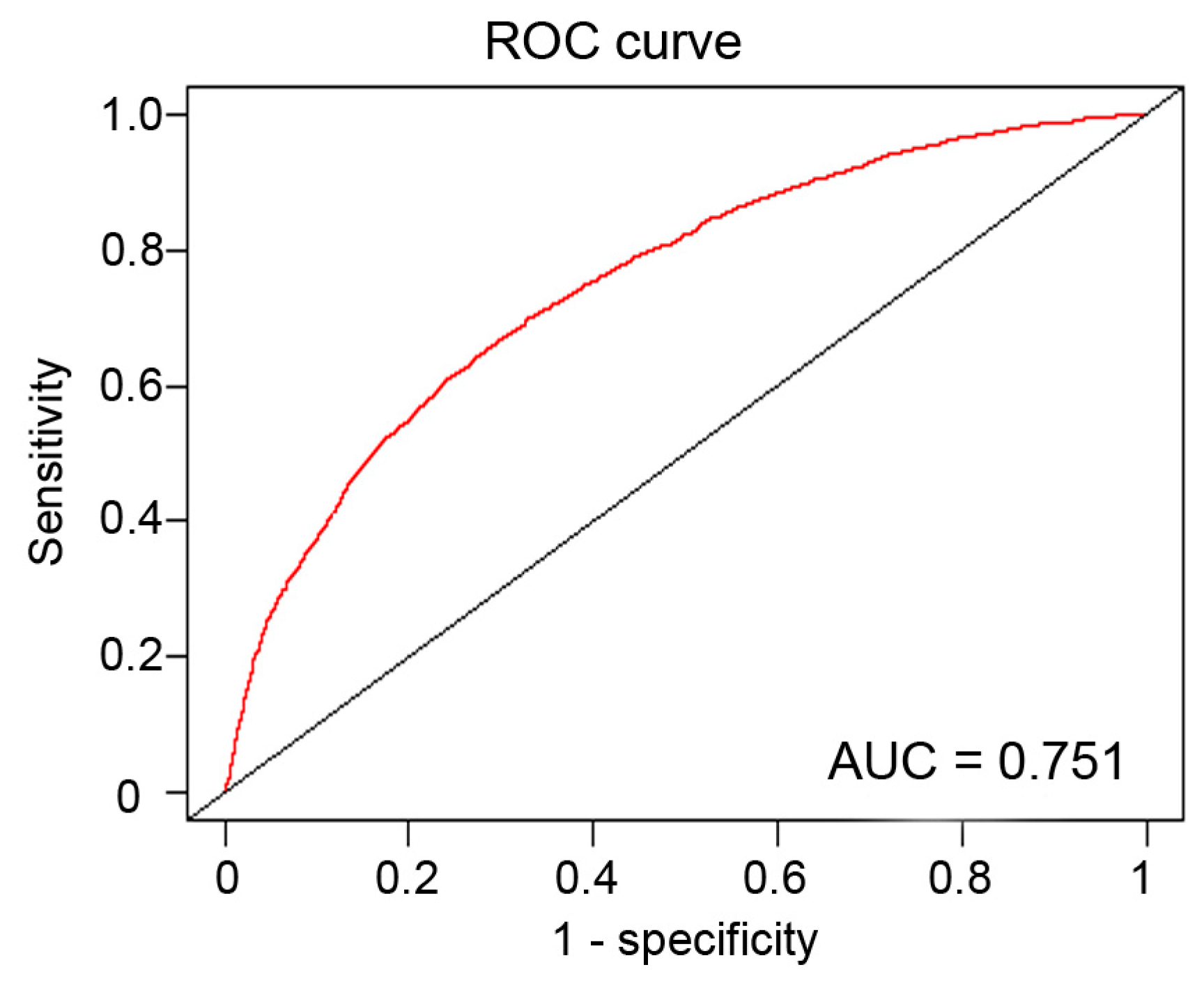
In the case of the climatic factors, disease status transition was negatively correlated with annual mean temperature (Bio01) and positively correlated with precipitation in the warmest quarter (Bio18; Table 3). The AUC value for the final multiple regression model was 0.751 (Figure 3), indicating a moderate predictive power.

4. Discussion

Previous studies have demonstrated that landscape configuration, such as habitat connectivity, can potentially influence the risk of infectious diseases [35,36]. However, these studies sometimes showed contradictory results about the role of habitat connectivity. In this study, we examined the effects of forest connectivity, as well as the effects of the host assemblage characteristics of local and neighboring counties, on the spatial spread of Lyme disease in the United States. We found that both the infection intensity of neighbors and local assemblage similarity had positive effects on the risk of disease spread. These two effects also depended on the level of forest connectivity, though forest connectivity itself did not play a significant role.
The spread of Lyme disease involves two processes: the dispersal potential of infected hosts/vectors and the establishment of infection [37]. Generally, the dispersal potential of infected hosts/vectors largely depends on the abundance of infected hosts/vectors [38]. Also, the probability of disease establishment seems to be positively correlated with the abundance of infected hosts [39]. Consistent with these statements, we found a strong positive relationship between the infection intensity of neighbors and disease spread. In heavily infected counties, the number of both infected ticks and hosts are expected to be high, which is able to enhance the chances that infected hosts or ticks move to disease-free counties or facilitate disease establishment. In addition, we found the effect of neighbor infection intensity depended on forest connectivity. With increasing connectivity, the effect of neighbor infection intensity became greater, increasing the risk of disease spread from neighboring counties.
Disease invasion and establishment may also depend on the suitability of new areas [38]. We found that the risk of disease spread positively correlated with the similarity between local and neighboring host assemblages. Due to host specificity of vectors and pathogens, these organisms are more likely to infect hosts that are ecologically or phylogenetically similar [21]. Therefore, disease is more likely to spread between assemblages that are similar and share common host species [40]. Additionally, similar host assemblages might indicate high similarity in habitat and resource availability, which can facilitate the adaptation of hosts and vectors to the new environments [38,41], thereby promoting disease establishment. Moreover, we found that the relationship between host assemblage similarity and disease spread also depends on forest connectivity. The effect size of the host assemblage similarity decreased with increasing forest connectivity Thus, host assemblage similarity is apparently less important when host species can move easily across county borders in well-connected habitats, and the transition in disease status can occur even when the host assemblage similarity is not very high.
For climatic factors, we found a negative correlation between annual mean temperature and the risk of Lyme spread, which is consistent with many previous studies [26,27]. However, as the mean temperature was highly correlated with other temperature-related variables (such as the maximum temperature of warmest month and the mean temperature in the warmest quarter), we cannot determine which variable is mechanistically most important. A general mechanism underlying this relationship may be desiccation, to which ticks, especially larvae and nymphs, are susceptible [42]. As temperature increases, the tick density may decrease due to desiccation, leading to a reduced risk of Lyme disease. The annual precipitation did not show a significant correlation with the risk of Lyme spread, while the precipitation in the warmest quarter (generally summer in the Northern Hemisphere) showed a positive relationship. Thus, summer precipitation might be a better predictor then annual precipitation. Indeed, summer precipitation is positively related to the abundance of blacklegged ticks in northwest Illinois [43]. In this case, the proposed mechanism is through a negative effect of summer drought on understory plants and leaf litter layer: more exposed and drier soils are expected to reduce tick survival and reproduction [43].
It is important to acknowledge some limitations associated with our study. For example, we used the data of reported human cases of Lyme disease, which might be underreported [26]. Additionally, the data we used offered only a “global” snapshot per county. Consequently, it was impossible for us to analyze if new cases in a previously uninfected county occurred along a border with an infected county. It was similarly impossible to take into account the mobility of infected people due to the lack of these data. Finally, the host distributions were obtained from the IUCN and did not take into account any possible changes (e.g., range shifts, expansions, or contractions) that occurred during the study period. Even though these data limitations may partly restrict our conclusions, our study still offers important new insights into the factors driving the spread of such a zoonotic disease. We are among the first to explore the interactions between habitat connectivity and characteristics of local and neighboring assemblages on disease expansion, and the results of our analyses demonstrate how important these interactions can be.

5. Conclusions

In this study, we explored the role of host assemblage characteristics and forest connectivity of local and neighboring counties in shaping Lyme disease expansion in the United States. Our results showed that the similarity between local and neighboring host assemblages and the infection intensity of neighbors had positive effects on the risk of disease expansion. Moreover, higher forest connectivity promoted the role of neighbor infection intensity and negated the role of host assemblage similarity. Our results, therefore, provide valuable new insights into the underlying interacting mechanisms that influence the spread of disease. Since factors related to disease spread do not function in isolation, future studies in this area should continue analyzing these interactions between ecologically relevant parameters.

Supplementary Materials

The following are available online at https://www.mdpi.com/2072-4292/11/20/2354/s1. Table S1: Results of univariate analyses (b, estimated coefficients and Z-statistics), Table S2: Correlations between candidate variables.

Author Contributions

Data curation, Y.X.G.W. and Y.X.; Formal analysis, Y.X.G.W. and Z.Y.X.H.; Investigation, Y.X.; Methodology, Y.X.G.W., K.D.M., Y.X., Z.Y.X.H. and W.F.d.B.; Supervision, Z.Y.X.H., K.D.M., H.H.T.P. and W.F.d.B.; Visualization, Y.X.G.W. and Y.X.; Writing—original draft, Y.X.G.W.; Writing—review & editing, K.D.M., Y.X., H.H.T.P., Z.Y.X.H. and W.F.d.B.

Funding

This research was funded by National Natural Science Foundation of China, grant number 31870400, 31500383, Chinese Scholarship Council grant number 201506190134, and a project by the Priority Academic Programme Development (PAPD) of Jiangsu Higher Education Institutions.

Conflicts of Interest

The authors declare no conflict of interest.

References

  1. Smith, D.L.; Lucey, B.; Waller, L.A.; Childs, J.E.; Real, L.A. Predicting the spatial dynamics of rabies epidemics on heterogeneous landscapes. Proc. Natl. Acad. Sci. USA 2002, 99, 3668–3672. [Google Scholar] [CrossRef] [PubMed] [Green Version]
  2. Estrada-Peña, A. The relationships between habitat topology, critical scales of connectivity and tick abundance. Ecography 2003, 26, 661–671. [Google Scholar] [CrossRef]
  3. Estrada-Peña, A.; Ostfeld, R.S.; Peterson, A.T.; Poulin, R.; de la Fuente, J. Effects of environmental change on zoonotic disease risk: An ecological primer. Trends Parasitol. 2014, 30, 205–214. [Google Scholar] [CrossRef] [PubMed]
  4. Kilpatrick, A.M.; Randolph, S.E. Drivers, dynamics, and control of emerging vector-borne zoonotic diseases. Lancet 2012, 380, 1946–1955. [Google Scholar] [CrossRef] [Green Version]
  5. Reisen, W.K. Landscape Epidemiology of Vector-Borne Diseases. Annu. Rev. Entomol. 2009, 55, 461–483. [Google Scholar] [CrossRef] [PubMed]
  6. Huang, Z.Y.X.; Van Langevelde, F.; Estrada-Pena, A.; Suzan, G.; De Boer, W.F.W.; Estrada-Peña, A.; Suzán, G.; De Boer, W.F.W. The diversity–disease relationship: Evidence for and criticisms of the dilution effect. Parasitology 2016, 143, 1075–1086. [Google Scholar] [CrossRef] [PubMed]
  7. Huang, Z.Y.X.; van Langevelde, F.; Prins, H.H.T.; de Boer, W.F. Dilution versus facilitation: Impact of connectivity on disease risk in metapopulations. J. Theor. Biol. 2015, 376, 66–73. [Google Scholar] [CrossRef]
  8. George Hess Disease in Metapopulation Models: Implications for Conservation. Ecology 1996, 77, 1617–1632. [CrossRef]
  9. Stapp, P.; Hartley, L.M.; Savage, L.T.; Antolin, M.F.; Reich, R.M. Climate, soils, and connectivity predict plague epizootics in black-tailed prairie dogs (Cynomys ludovicianus). Ecol. Appl. 2011, 21, 2933–2943. [Google Scholar]
  10. Keeling, M.J. Metapopulation moments: Coupling, stochasticity and persistence. J. Anim. Ecol. 2000, 69, 725–736. [Google Scholar] [CrossRef]
  11. Turney, S.; Gonzalez, A.; Millien, V. The negative relationship between mammal host diversy and Lyme disease incidence strengthens through time. Ecology 2014, 95, 3244–3250. [Google Scholar] [CrossRef]
  12. Steere, A.C.; Coburn, J.; Glickstein, L.; Steere, A.C.; Coburn, J.; Glickstein, L. The emergence of Lyme disease. J. Clin. Invest. 2004, 113, 1093–1101. [Google Scholar] [CrossRef] [PubMed] [Green Version]
  13. Diuk-Wasser, M.A.; Gatewood, A.G.; Cortinas, M.R.; Yaremych-Hamer, S.; Tsao, J.; Kitron, U.; Hickling, G.; Brownstein, J.S.; Walker, E.; Piesman, J.; et al. Spatiotemporal patterns of host-seeking Ixodes scapularis nymphs (Acari: Ixodidae) in the United States. J. Med. Entomol. 2006, 43, 166–176. [Google Scholar] [CrossRef] [PubMed]
  14. Guerra, M.; Walker, E.; Jones, C.; Paskewitz, S.; Roberto Cortinas, M.; Ashley Stancil, L.B.; Bobo, M.; Kitron, U. Predicting the risk of Lyme disease: Habitat suitability for Ixodes scapularis in the north central United States. Emerg. Infect. Dis. 2002, 8, 289–297. [Google Scholar] [CrossRef] [PubMed]
  15. Cheng, A.; Chen, D.; Woodstock, K.; Ogden, N.H.; Wu, X.; Wu, J. Analyzing the potential risk of climate change on lyme disease in Eastern Ontario, Canada using time series remotely sensed temperature data and tick population modelling. Remote Sens. 2017, 9, 609. [Google Scholar] [CrossRef]
  16. Hamer, S.A.; Tsao, J.I.; Walker, E.D.; Hickling, G.J. Invasion of the Lyme disease vector Ixodes scapularis: Implications for Borrelia burgdorferi endemicity. Ecohealth 2010, 7, 47–63. [Google Scholar] [CrossRef]
  17. Lee, X.; Coyle, D.R.; Johnson, D.K.H.; Murphy, M.W.; McGeehin, M.A.; Murphy, R.J.; Raffa, K.F.; Paskewitz, S.M. Prevalence of Borrelia burgdorferi and Anaplasma phagocytophilum in Ixodes scapularis (Acari: Ixodidae) Nymphs Collected in Managed Red Pine Forests in Wisconsin. J. Med. Entomol. 2014, 51, 694–701. [Google Scholar] [CrossRef]
  18. Eisen, R.J.; Eisen, L.; Beard, C.B. County-scale distribution of Ixodes scapularis and Ixodes pacificus (Acari: Ixodidae) in the continental United States. J. Med. Entomol. 2016, 53, 349–386. [Google Scholar] [CrossRef]
  19. Watts, E.J.; Palmer, S.C.F.; Bowman, A.S.; Irvine, R.J.; Smith, A.; Travis, J.M.J. The effect of host movement on viral transmission dynamics in a vector-borne disease system. Parasitology 2009, 136, 1221–1234. [Google Scholar] [CrossRef]
  20. Guernier, V.; Hochberg, M.E.; Guégan, J.F.F. Ecology drives the worldwide distribution of human Diseases. PLoS Biol. 2004, 2, e141. [Google Scholar] [CrossRef]
  21. Esser, H.J.; Herre, E.A.; Blüthgen, N.; Loaiza, J.R.; Bermúdez, S.E.; Jansen, P.A. Host specificity in a diverse Neotropical tick community: An assessment using quantitative network analysis and host phylogeny. Parasites Vectors 2016, 9, 1–14. [Google Scholar] [CrossRef] [PubMed]
  22. Yu, P.; Li, Y.; Xu, B.; Wei, J.; Li, S.; Dong, J.; Qu, J.; Xu, J.; Huang, Z.Y.X.; Ma, C.; et al. Using satellite data for the characterization of local animal reservoir populations of Hantaan virus on the Weihe Plain, China. Remote Sens. 2017, 9, 1076. [Google Scholar] [CrossRef]
  23. Polo, G.; Labruna, M.B.; Ferreira, F. Satellite hyperspectral imagery to support tick-borne infectious diseases surveillance. PLoS ONE 2015, 10, 1–12. [Google Scholar] [CrossRef] [PubMed]
  24. Wimberly, M.C.; Baer, A.D.; Yabsley, M.J. Enhanced spatial models for predicting the geographic distributions of tick-borne pathogens. Int. J. Health Geogr. 2008, 7, 1–14. [Google Scholar] [CrossRef] [PubMed]
  25. Altizer, S.; Dobson, A.; Hosseini, P.; Hudson, P.; Pascual, M.; Rohani, P. Seasonality and the dynamics of infectious diseases. Ecol. Lett. 2006, 9, 467–484. [Google Scholar] [CrossRef] [PubMed] [Green Version]
  26. Killilea, M.E.; Swei, A.; Lane, R.S.; Briggs, C.J.; Ostfeld, R.S. Spatial dynamics of Lyme sisease: A review. Ecohealth 2008, 5, 167–195. [Google Scholar] [CrossRef]
  27. Tran, P.M.; Waller, L. Effects of landscape fragmentation and climate on lyme disease incidence in the Northeastern United States. Ecohealth 2013, 10, 394–404. [Google Scholar] [CrossRef]
  28. Fick, S.; Hijmans, R. Worldclim 2: New 1-km spatial resolution climate surfaces for global land areas. Int. J. Climatol. 2017, 37, 4302–4315. [Google Scholar] [CrossRef]
  29. Dornelas, M.; Gotelli, N.J.; McGill, B.; Shimadzu, H.; Moyes, F.; Sievers, C.; Magurran, A.E. Assemblage time series reveal biodiversity change but not systematic loss. Science 2014, 344, 296–299. [Google Scholar] [CrossRef]
  30. IUCN. The IUCN Red List of Threatened Species. Version 2015-3; IUCN: Gland, Switzerland, 2015. [Google Scholar]
  31. Dixon, P. VEGAN, a package of R functions for community ecology. J. Veg. Sci. 2003, 14, 927–930. [Google Scholar] [CrossRef]
  32. Zuur, A.F.; Ieno, E.N.; Elphick, C.S. A protocol for data exploration to avoid common statistical problems. Methods Ecol. Evol. 2010, 1, 3–14. [Google Scholar] [CrossRef]
  33. Gray, J.S.; Dautel, H.; Estrada-Peña, A.; Kahl, O.; Lindgren, E. Effects of climate change on ticks and tick-borne diseases in Europe. Interdiscip. Perspect. Infect. Dis. 2009, 2009, 1–12. [Google Scholar] [CrossRef] [PubMed]
  34. Medlock, J.M.; Leach, S.A. Effect of climate change on vector-borne disease risk in the UK. Lancet Infect. Dis. 2015, 15, 721–730. [Google Scholar] [CrossRef]
  35. Lambin, E.F.; Tran, A.; Vanwambeke, S.O.; Linard, C.; Soti, V. Pathogenic landscapes: Interactions between land, people, disease vectors, and their animal hosts. Int. J. Health Geogr. 2010, 9, 54. [Google Scholar] [CrossRef]
  36. Estrada-Peña, A. Diluting the dilution effect: A spatial Lyme model provides evidence for the importance of habitat fragmentation with regard to the risk of infection. Geospat. Health 2009, 3, 143–155. [Google Scholar] [CrossRef]
  37. White, L.A.; Forester, J.D.; Craft, M.E. Disease outbreak thresholds emerge from interactions between movement behavior, landscape structure, and epidemiology. Proc. Natl. Acad. Sci. USA 2018, 115, 7374–7379. [Google Scholar] [CrossRef] [Green Version]
  38. Watts, A.G.; Saura, S.; Jardine, C.; Leighton, P.; Werden, L.; Fortin, M.J. Host functional connectivity and the spread potential of Lyme disease. Landsc. Ecol. 2018, 33, 1925–1938. [Google Scholar] [CrossRef]
  39. Lloyd-Smith, J.O.; Cross, P.C.; Briggs, C.J.; Daugherty, M.; Getz, W.M.; Latto, J.; Sanchez, M.S.; Smith, A.B.; Swei, A. Should we expect population thresholds for wildlife disease? Trends Ecol. Evol. 2005, 20, 511–519. [Google Scholar] [CrossRef]
  40. Fountain-Jones, N.M.; Pearse, W.D.; Escobar, L.E.; Alba-Casals, A.; Carver, S.; Davies, T.J.; Kraberger, S.; Papeş, M.; Vandegrift, K.; Worsley-Tonks, K. Towards an eco-phylogenetic framework for infectious disease ecology. Biol. Rev. 2018, 93, 950–970. [Google Scholar] [CrossRef]
  41. Hofmeester, T.R.; Prins, H.H.T.; Coipan, E.C.; Sprong, H.; van Wieren, S.E.; Takken, W. Few vertebrate species dominate the Borrelia burgdorferi s.l. life cycle. Environ. Res. Lett. 2016, 11, 043001. [Google Scholar] [CrossRef]
  42. Ostfeld, R.S.; Canham, C.D.; Oggenfuss, K.; Winchcombe, R.J.; Keesing, F. Climate, deer, rodents, and acorns as determinants of variation in Lyme disease risk. PLoS Biol. 2006, 4, e145. [Google Scholar] [CrossRef] [PubMed]
  43. Jones, C.J.; Kitron, U.D. Populations of Ixodes scapularis (Acari: Ixodidae) are modulated by drought at a Lyme disease focus in illinois. J. Med. Entomol. 2000, 37, 408–415. [Google Scholar] [CrossRef] [PubMed]
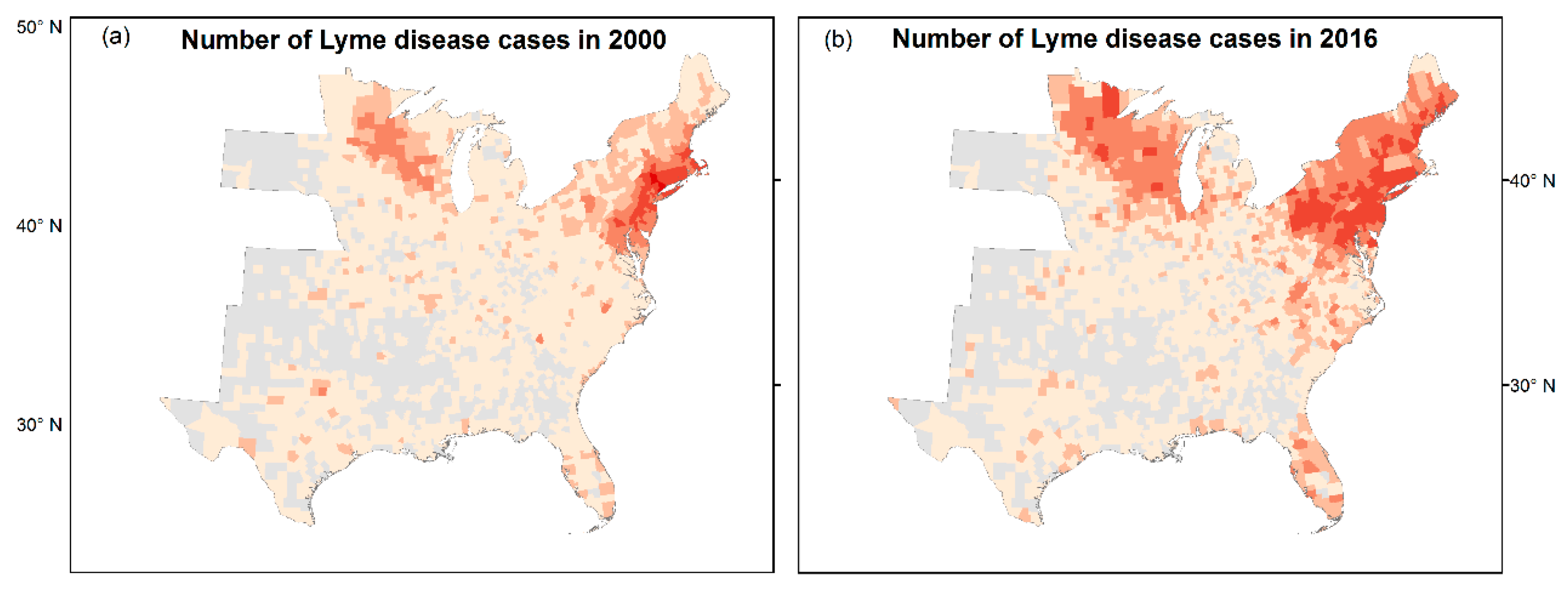
Figure 1. The distribution of Lyme disease cases at the county level in (a) 2000 and (b) 2016 in the 35 states of the United States with established or reported Ixodes scapularis populations.
Remotesensing 11 02354 g001
Figure 2. The interaction effects of forest connectivity with (a) the infection intensity of neighboring counties and (b) the similarity of local host assemblage on the predicted probability that a disease-free county shifted to infected. Red indicates low forest connectivity; blue indicates high forest connectivity.
Remotesensing 11 02354 g002
Figure 3. ROC (receiver operating characteristic) curve and AUC (area under ROC curve) value for the selected multiple regression model explaining the probability of county-level disease status transition from Lyme disease free to infected.
Remotesensing 11 02354 g003
Table 1. Hypotheses and explanatory variables used in the analyses modelling the spatial spread of Lyme cases in the United States.
AbbreviationVariableHypotheses
Local assemblage similarityThe similarity of local host assemblage with neighboring countiesCounties with high similarity of host assemblage with infected neighbors would have a higher risk of disease spread
Forest connectivityForest habitat connectivity between local county and neighboring countyCounties with high connectivity with infected neighbors would have a higher risk.
Neighbor infection intensity Number of Lyme cases reported in neighboring counties in the previous yearCounties close to heavily infected neighbors would have a higher risk.
Bio01, Bio05, Bio10 1Temperature-related variables [28]Higher temperature and precipitation support tick establishment, tick survival, and contribute to the expansion of the distribution range of ticks [33,34]; however, a higher temperature can also decrease tick density by dehydrating ticks [26,27].
Bio12, Bio13, Bio14, Bio16, Bio18 1Precipitation-related variables [28]
Human populationHuman population size Counties with high population density may have a high disease risk.
1 Bio01: mean annual temperature; Bio05: maximum temperature of warmest month; Bio10: mean temperature of warmest quarter; Bio12: annual precipitation; Bio13: precipitation of wettest month; Bio16: precipitation of wettest quarter and Bio18: precipitation of warmest quarter
Table 2. Summary of numbers and ratio of transition from disease-free to infected county from 2000~2016.
Time PeriodNo. of Counties that Remained Disease-FreeNo. of Counties that Transitioned from a Disease-Free to Infected State% of the Total Number of Counties that Became Infected
2000–200161615620%
2001–200249516928%
2002–200357615521%
2003–200455513720%
2004–200555315622%
2005–200651412620%
2006–200745018629%
2007–200851017125%
2008–200949016525%
2009–201048413422%
2010–201144113724%
2011–201244319831%
2012–201340316731%
2013–201442515827%
2014–201539517130%
2015–201639817130%
Mean ± S.D.484 ± 64.9160 ± 18.725% ± 4%
Table 3. Summary of results (Adjusted Odds Ratio, AOR, with their 95% confidence intervals (CI) and P values) of the final regression model, correlated with the probability of county-level disease status transition from Lyme disease free to Lyme disease present.
VariablesAOR95% CIP
Neighbor infection intensity1.49[1.40, 1.61]<0.001
Forest connectivity1.08[1, 1.15]0.05
Local assemblage similarity1.15[1.08, 1.22]<0.001
Neighbor infection intensity * Habitat connectivity1.10[1.02, 1.17]0.01
Local assemblage similarity * Habitat connectivity0.90[0.85, 0.96]0.01
Mean temperature0.43[0.40, 0.46]<0.001
Precipitation of warmest quarter1.27[1.20, 1.38]<0.001