Drawback in the Change Detection Approach: False Detection during the 2018 Western Japan Floods

Abstract

Synthetic aperture radar (SAR) images have been used to map flooded areas with great success. Flooded areas are often identified by detecting changes between a pair of images recorded before and after a certain flood. During the 2018 Western Japan Floods, the change detection method generated significant misclassifications for agricultural targets. To evaluate whether such a situation could be repeated in future events, this paper examines and identifies the causes of the misclassifications. We concluded that the errors occurred because of the following. (i) The use of only a single pair of SAR images from before and after the floods. (ii) The unawareness of the dynamics of the backscattering intensity through time in agricultural areas. (iii) The effect of the wavelength on agricultural targets. Furthermore, it is highly probable that such conditions might occur in future events. Our conclusions are supported by a field survey of 35 paddy fields located within the misclassified area and the analysis of Sentinel-1 time series data. In addition, in this paper, we propose a new parameter, which we named “conditional coherence”, that can be of help to overcome the referred issue. The new parameter is based on the physical mechanism of the backscattering on flooded and non-flooded agricultural targets. The performance of the conditional coherence as an input of discriminant functions to identify flooded and non-flooded agricultural targets is reported as well.

1. Introduction

Floods are natural phenomena that can perturb ecosystems and societies [1,2]. Microwave remote sensing is extremely useful for post-disaster analysis of floods for two reasons: First, microwaves can penetrate clouds, which are almost certainly present during heavy rainfall events. Second, there is a clear physical mechanism for backscattering in waterbodies, that is, specular reflection. There are several methods to trace the flooded area from microwave remote sensing. Schumann and Moller [3] provided a comprehensive review of the role of microwave remote sensing on flood inundations. Their study focuses on the different potential conditions, such as mapping inundation at floodplains, coastal shorelines, wetlands, forest, and urban areas. For each case, the limitations and advantages of microwaves images are drawn. Nakmuenwai et al. [4] proposed a framework to identify flood-based water areas along the Chao Phraya River basin of central Thailand, an area were floods occur almost every year. Their study established an inventory of permanent waterbodies within the Chao Phraya River basin. Then, for an arbitrary SAR image, local thresholds are computed using the inventory of waterbodies as references. The architecture of the proposed network is independent of the satellite acquisition condition and normalization was not necessary. Liu and Yamazaki [5] performed a similar approach to map the waterbodies in open areas due to the 2015 Kanto and Tohoku torrential rain in Japan. It was pointed out, however, that a thresholding method applied over the backscattering intensity has a poor performance in urban areas. The combined effect of the specular reflection and double-bounce backscattering mechanism produces high backscattering intensity. Thus, Liu and Yamazaki [5] applied the threshold over the difference of backscattering between a pair of SAR images taken before and after the referred flood. Boni et al. [6] introduced a prototype system for flood monitoring in near-real-time. Instead of using an inventory of water body as a reference, they used an automatic procedure to find subimages with bimodal distribution and used them to set the threshold. The novelty in this study is the use of numerical simulation to forecast floods and to request earlier satellite activation. When multitemporal SAR data is available, Pulvirenti et al. [7] proposed a methodology based on image segmentation and electromagnetic models to monitor inundations. Pierdicca et al. [8] used the irrigation activities in agricultural targets to test whether COSMO-Skymed SAR data is able to detect vegetation with water beneath it. The aim of the study is to detect flooded vegetation areas in future events. Pulvirenti et al. [9] tackled the problem of discriminate flooded and non-flooded vegetation areas by applying a supervised machine learning classifier on a segmentation-based classification. In their study, a theoretical backscattering model was used as training data. However, a proper theoretical model requires information on land cover map as complementary input. Although currently polarimetric SAR images are not usually available for early disaster purposes, Sui et al. [10] performed a study of its use together with a digital elevation model (DEM) and ancillary data. Arnesen et al. [11] combined L-band SAR images, optical images, and SRTM data to monitor the seasonal variations of flood extent at the Curuai Lake floodplain, in the Amazon River, Brazil.

Most of these studies are based on similar principles, one of which is the detection of waterbodies through the identification of areas with low backscattering intensity. For the case of vegetation, however, flooded vegetation may give rise to large backscatter intensities, due to the joint effect of specular reflection of a smooth water surface and the double bounce effect of plant stalks. However, this joint effect is intimately connected to the frequency bands. A frequency associated with a short wavelength, for instance, in the X-band, is able to interact with the plant stalks. On the other hand, larger wavelengths, such as those in the L-band, may not interact with thin or low-dense plant stalks. Another important principle often used in many studies is the comparison of waterbodies observed in a pair of images taken before (pre-event) and after (post-event) an arbitrary flood event. When the temporal baseline between the referred images is sufficiently short, it is assumed that most of the changes observed are effects of the disaster. This procedure is commonly referred to as change detection, and it is frequently used to analyze large-scale disasters. For the case of floods, change detection is used to remove permanent waterbodies from those caused by the disaster.

An inevitable issue in the change detection approach is that changes produced by other factors within the temporal baseline will be detected as well. This is the main reason why a change detection-based damage map is performed with a pair of images with the shortest available temporal baseline. An important constraint is the availability of a pre-event image. To the best of our experience, a temporal baseline from few months to about a year performs fairly well to identify damages in urban areas [12,13,14,15,16,17,18]. However, other types of land use may exhibit constant and systematic changes through time. Areas devoted to agricultural activities are such examples. Based on seasonal changes, the referred areas may contain bare soil, water, and/or vegetation. Previous studies have shown that these periodical changes can be detected from remote sensing imagery. Rosenqvist [19], for instance, performed an extensive study of the dynamics of the backscattering intensity in agricultural targets in Malaysia. The referred study used microwave images recorded by JERS-1, a Japanese satellite with L-band sensor. Five images, recorded during the soil preparation, initial reproduction, budding, harvesting, and soil preparation (after harvesting), were analyzed. Studies of agricultural targets using other frequency bands have been performed also [20,21].

The application of change detection to map the effect of a flood in agricultural targets is therefore more complicated that its application in urban areas. Previous studies have stated that their results might contain changes produced by the flood and agricultural activities. Liu and Yamazaki [5] reported that the change of waterbodies included large paddy fields flooded for irrigation purposes, which could not be removed. Boni et al. [6] pointed out it is necessary to include a pre-event image recorded a few days before the flood to successfully remove all the permanent waters, including those from the agricultural activities. However, this is usually not available. To the best of our knowledge, there is no report of the severity of this issue, namely, the inability to discriminate changes of waterbodies from the flood and those from agricultural activities.

Thus, the aim of this study is to report on the above issue during our analysis of the 2018 heavy rainfall that occurred in western Japan and to provide a potential solution. The next section describes the region of interest, the available dataset during the early disaster response, and the data collected on subsequent days, such as additional microwave imagery, governmental reports, and the field survey. Section 3 reports the current approaches to map flooded areas. Their limitations to discriminate flooded and non-flooded agricultural targets are highlighted. Moreover, a new parameter is proposed to improve the identification of flooded and non-flooded agricultural targets. The results of the proposed metric and the performance of machine learning classification algorithms calibrated with the new parameter is reported in Section 4. Additional comments are provided in Section 5. Finally, our conclusions are reported in Section 6.

2. Dataset and Case Study

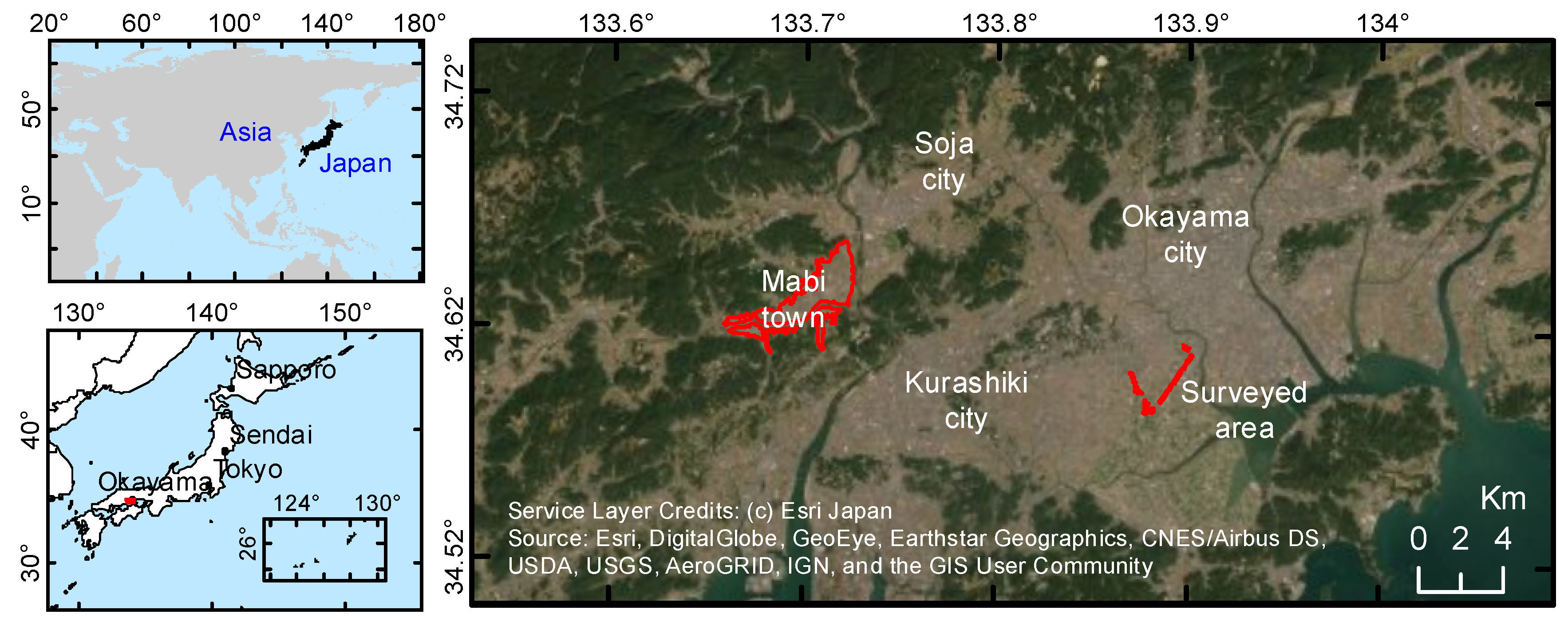
2.1. The 2018 Western Japan Floods

Beginning on 5 July 2018, heavy rainfall occurred in western Japan. A detailed report can be found in [22], although a summary follows. The cause of the heavy rainfall was attributed to the convergence of a weather front and the Typhoon No. 7. The total rainfall between 28 June and 8 July was 2–4 times the average monthly values for July. As of 2 August 2018, 220 casualties, nine missing persons, and 381 injuries had been reported due to the floods, mainly in Hiroshima and Okayama Prefectures. Furthermore, 9663 houses were partially or completely collapsed, 2579 were partially damaged, 13,983 houses were flooded to the first floor, and 20,849 houses were flooded below the first floor. Figure 1 shows the geographical location of the region of interest (ROI) of this study, which is located in the prefecture of Okayama. It includes the cities of Kurashiki, Okayama, and Soja. Within Kurashiki city is located the town of Mabi, the most affected area in Okayama Prefecture during the heavy rainfall.

2.2. The Advance Land Observing Satellite-2 (ALOS-2)

In the aftermath of the 2018 heavy rainfall event, the ALOS-2 performed observations on the affected areas for early disaster response purposes. The ALOS-2 system was developed by the Japan Aerospace Exploration Agency (JAXA). The ALOS-2 hosts an L-band SAR system, named PALSAR-2, that is capable of right and left looking imaging with an incident angle range of 8°–70°. The revisit time of ALOS-2 is 14 days. PALSAR-2 is able to operate in three different modes: (i) spotlight mode, with azimuth and range resolution of 1 m and 3m, respectively; (ii) stripmap mode, which has the ultrafine, high-sensitivity, and fine submodes; (iii) and ScanSAR mode, with low resolution for large swaths. Figure 2a shows a RGB color composite of a pair of images acquired on 14 April 2018 (R), and 7 July 2018 (G and B) in the ROI. The images are in Stripmap-ultrafine mode, which has a ground resolution of 3 m, and both are in HH polarization. The gray tones are areas where the backscattering intensity remain unchanged, whereas the red tones indicated the areas where the backscattering intensity decreased.

The two referred images were provided at the early stage of the disaster. Later on, another pre-event image with the same acquisition conditions was requested for this study. The third image was recorded on 3 March 2017. Note that all the images were radiometrically calibrated, speckle filtered, and terrain corrected.

2.3. The Sentinel-1 Satellite

To reveal the impact of the irrigation and seasonal changes, annual variations of backscattering at the agriculture targets were investigated using Sentinel-1 data. The Sentinel-1 constellation, operated within the European Commission’s Copernicus program, can provide dual-polarized C-band SAR images every six days [23]. Annual changes in backscattering from paddy fields were analyzed using ground range detected (GRD) images taken from 1 January 2017 to 31 December 2018. Note that only the images taken from the descending path under VV polarization were extracted to reduce the effects of the acquisition conditions. As a result, a total of 58 SAR images were selected for this study. The preprocessing of these images consists of three steps: orbit correction, calibration, and geometric terrain correction. First, orbit state vectors were modified using supplementary orbit information provided by the Copernicus Precise Orbit Determination Service. This modification has a high influence on the quality of several preprocessing steps. Second, brightness was converted into backscattering coefficient, which represents the radar intensity per unit area in the ground range. Third, geometric distortion derived from varying terrain were corrected using digital elevation data provided by the Shuttle Radar Topographic Mission.

2.4. Truth Data

Currently, the Geospatial Information Authority of Japan (GSI) provides data related to the effects of the floods [24]. A series of derived products are available in the referred data base, such as orthophotos taken before and after the disaster, collapsed areas map, inundation range, estimation of inundation depth, and digital elevation map. Figure 1 illustrates the extent of the flooded area in Mabi-town. It is worth pointing out that the area delineated by GSI was performed using photos and videos only; and thus its accuracy was not confirmed.

As seen in Figure 2a, the flooded area in Mabi town exhibit a reduction of the backscattering intensity, which is expressed as red tones. However, many other areas exhibit the same pattern as well. A closer look revealed that most of those areas are used for agriculture activities. Therefore, to complement the data provided by GSI, a field survey was performed on 25 July, 18 days after the recording of the post-event image. The location of the surveyed paddy fields is shown in Figure 1 and a closer look is shown in Figure 3. A total of 35 agricultural fields were inspected (Figure 3a). There was no evidence of flooding, and direct communication with the inhabitants confirmed that no flooding occurred in the surveyed area. Furthermore, it was found that the plants were in their early stage of growth, and a layer of water was present in most of the fields (Figure 3b,c).

3. Methods

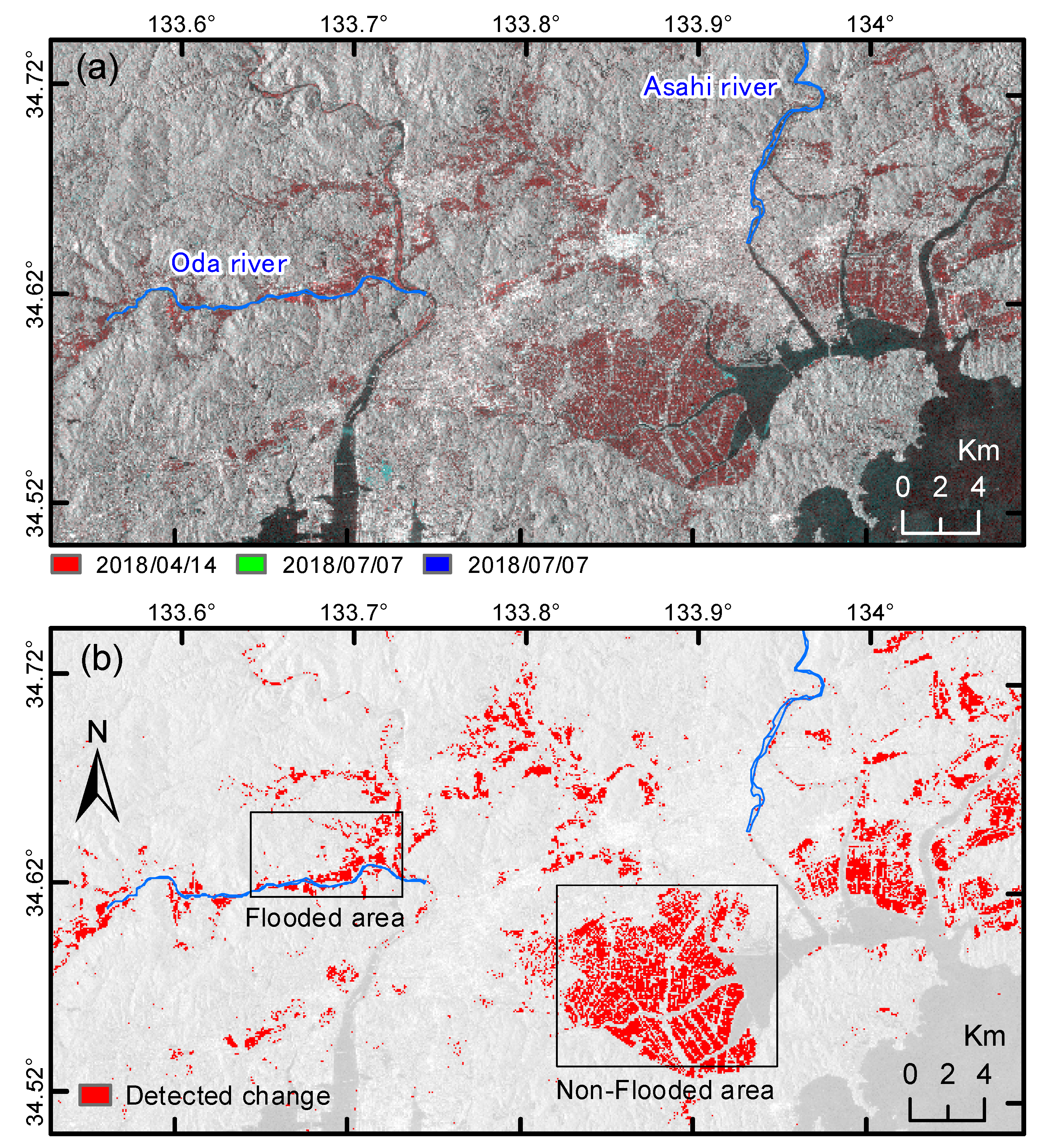
3.1. Current Practice for Flood Mapping

3.1.1. Intensity Thresholding

This section begins reproducing one of the simplest approaches to estimate flooded areas in the ROI, that is, identifying areas with low backscattering values in the ALOS-2 SAR imagery. To define a proper threshold, permanent waterbodies from the Asahi and Oda rivers, shown as blue polygons in Figure 2, are employed as references. As pointed out in [4], by using water body references from the same images, there is no effect of the acquisition conditions of the images (i.e., incident angle, satellite path, etc.) in the results. A threshold of −16 dB for the sigma naught backscattering was set, and the waterbodies were identified in both the pre- and post-event images with the shortest time baseline; that is, the images recorded on April and July 2018. The permanent waterbodies in the post-event image were removed using the waterbodies at the pre-event image. Then, the erosion and dilatation operator, with window size of $3\times 3$, were applied in order to remove small objects. Figure 2b depicts the estimated flooded areas based on changes in waterbodies. As stated previously, there are several systematic procedures to set a threshold value. It was found, at least in this event, that slight modifications to the threshold value (−16 dB) did not change the overall flood map significantly. A similar flood map for Okayama Prefecture for the same event is reported in [25]. In Figure 2b, two areas are highlighted by black rectangles. The rectangle at the left side is located in Mabi-town, hereafter referred to as the F-area. It contains the flooded area mapped by GSI, which was confirmed as flooded by the media immediately after the disaster occurred. The second rectangle, hereafter referred as NF-area, corresponds to an area mainly devoted to agricultural activities. Note that the surveyed agricultural fields are located in the NF-area. According to the flood map (Figure 2b), the NF-area was severely affected. However, it came to our attention that there was no report of damage in this area, neither from the government nor the media. Recall, during the field survey, that the inhabitants also confirmed the NF-area was not flooded. Furthermore, a closer look at the SAR images showed dark rectangular areas distributed in a rather uniform way (Figure 3a). Therefore, it is concluded that these areas contained waterbodies used for agricultural activity and not caused by flooding. For the sake of clarity, fields that contain waterbodies due to agricultural activities are referred as “non-flooded agricultural targets”. Likewise, agricultural fields covered with waterbodies produced by the flood are interpreted as “flooded agricultural targets”. Specular reflection was indeed the main backscattering mechanism in the NF-area. Double bouncing did not occur for two reasons: the very thin stalks of the plants and the rather large L-band wavelength (15–30 cm). The backscattering sigma naught (${\sigma }_0$) intensity of the flooded area in Mabi town, and the surveyed paddy fields were measured and shown in Figure 4. The range of the backscatter intensity in the flooded agricultural fields was almost the same as that of the non-flooded agricultural fields. Therefore, it is expected that a pixel-based classification approach will produce incorrect results. Some of the agricultural fields were inactive (F07, F10, F29, F30, F34, and F35); that is, we only observed bare soil by the time of the survey, and the associated backscattering intensities were larger than those of the remaining fields. The large intensity shown for field F19 was attributed to artifacts of double bouncing due to a nearby building.

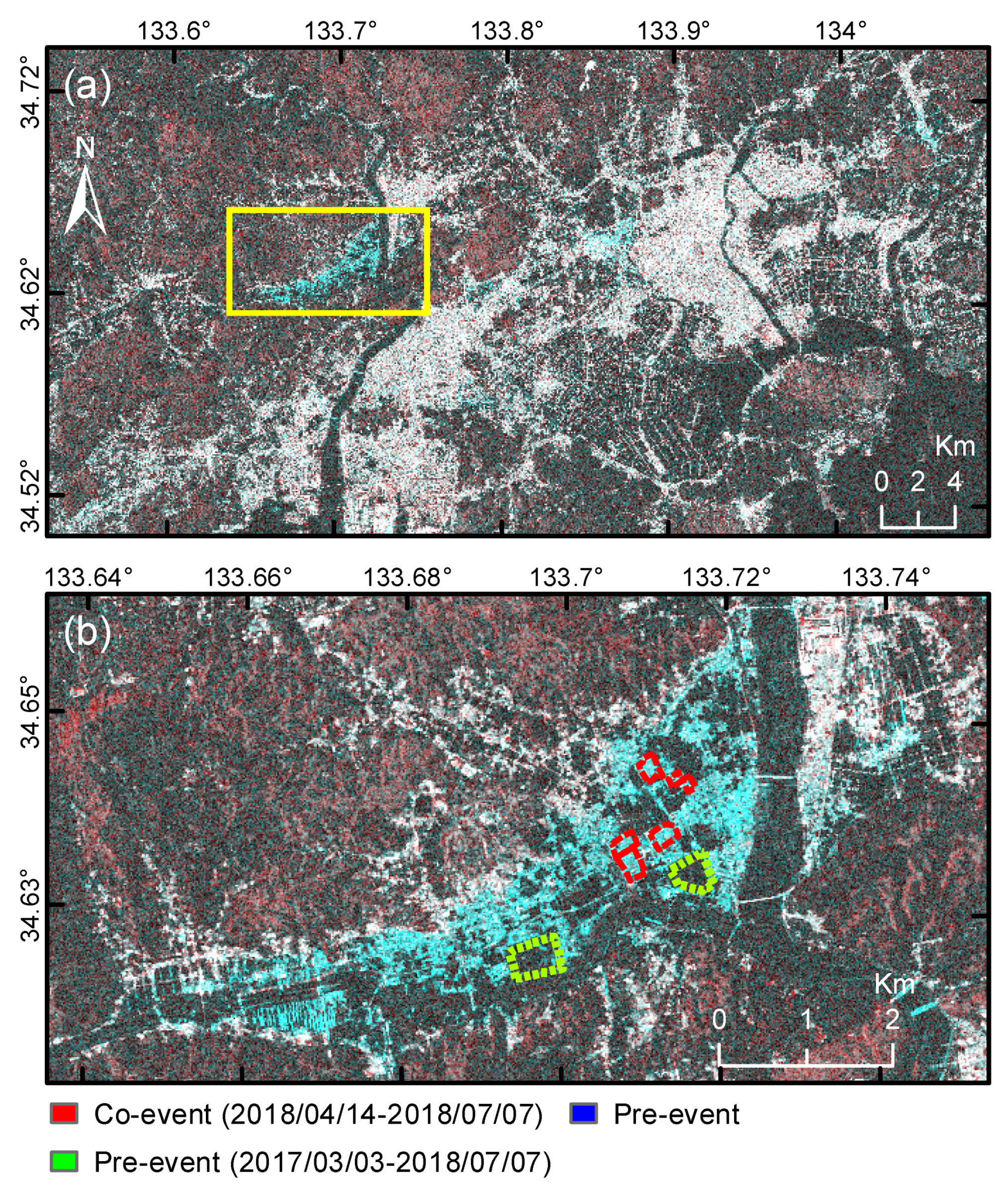
3.1.2. Coherence Approach

The use of complex coherence is another approach that has been frequently used in recent years to map damaged areas [5,18]. Coherence is computed from a pair of complex SAR data using the following expression,

$$\gamma =\frac{|{\sum }_{(i,j)}{I}_{i,j}^{pre}{I_{i,j}^{pos}}^{\ast }|}{\sqrt{{\sum }_{(i,j)}{I}_{i,j}^{pre}{I_{i,j}^{pre}}^{\ast }{\sum }_{(i,j)}{I}_{i,j}^{pos}{I_{i,j}^{pos}}^{\ast }}}$$

(1)

where $I_{i,j}^{pre}$ denotes the complex backscattering of the pre-event SAR image, $I_{i,j}^{pos}$ is the complex backscattering of the post-event SAR image, and * denotes the complex conjugate. Coherence tends to be large in urban areas, unless significant changes have occurred, such as the condition immediately after a large-scale disaster. In urban areas surrounded by dense vegetation, a single coherence computed from pre- and post-event SAR imagery might not be sufficient, because vegetation also exhibits low coherence. This pitfall can be overcome with a land cover map or an additional coherence image computed from two pre-event images. This approach was evaluated in the present study as well. The pre-event coherence were computed with the two pre-event SAR images (i.e., the images recorded on March 2017 and April 2018). The co-event coherence was computed with the post-event and the pre-event SAR images that have the shortest temporal baseline (i.e., the images recorded on April and July 2018). Figure 5 depicts the RGB color composite constructed from both coherence images (R: co-event coherence; G and B: pre-event coherence). The cyan tones are areas where the pre-event coherence dominates, which is mostly observed in urban areas affected by the flood. See the red polygons in Figure 5b for instance. The white tones are areas where both the pre-event and co-event have high values. This pattern is observed in non-flooded urban areas. It is promising to observe the NF-area exhibit a clear different tone than that shown in the F-area. The non-flooded agricultural targets have low values at both the pre-event and co-event coherence, which is reflected by dark tones. However, a closer look revealed that flooded agricultural targets exhibit dark tones as well. For instance, see the green polygons in Figure 5b. Therefore, using coherence-based change detection, floods in agriculture targets cannot be identified. To confirm this conclusion, Figure 6 depicts a scatter plots of flooded agricultural areas, flooded urban areas, and non-flooded agricultural areas. Each scatter plot were constructed from 10,000 samples randomly selected from the polygons shown in Figure 3a,b. It is clear that there is a significant overlapping between samples from flooded (Figure 6a) and non-flooded (Figure 6c) agriculture targets.

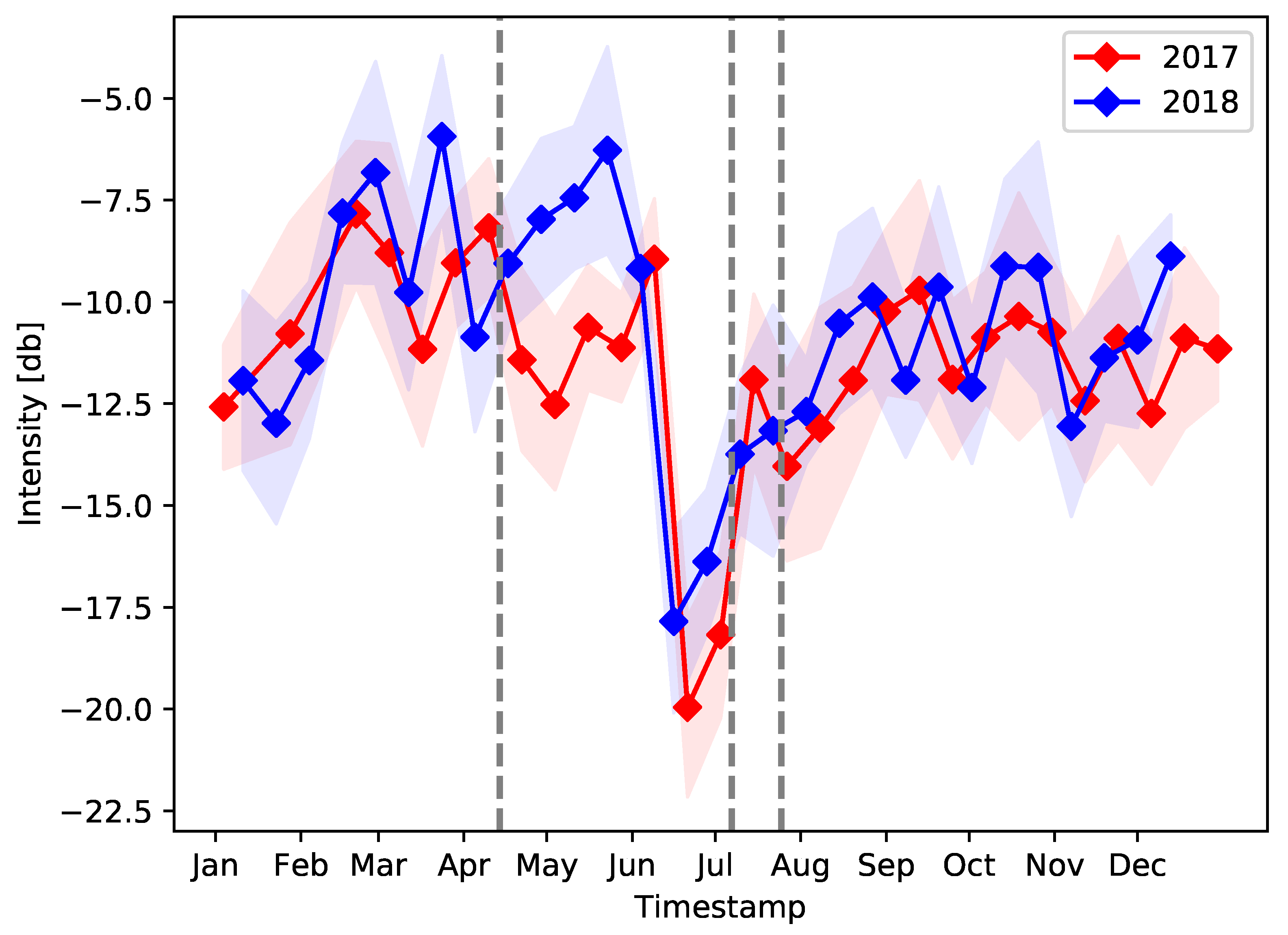
3.2. Backscattering Dynamics of Agriculture Targets

The evidence from the field survey demonstrated that the paddy fields were filled with water by the time the post-event image was recorded. Furthermore, Figure 2b suggests that such waterbodies were not present by the time the pre-event image was recorded. However, there is not conclusive evidence. If the pre-event image was taken before irrigation, the change detection approach would include irrigation changes and flood damage. Before starting irrigation and transplanting, the backscattering response from paddy fields is generally dominated by surface scattering of bare soil.

Fortunately, agriculture activities are associated with the seasons. Thus, the variation of the backscattering can be modeled as a periodic signal with a period of a year. Figure 7 illustrates the variation of the averaged backscattering intensity through the years 2017 (red line) and 2018 (blue line), corresponding to the surveyed paddy field F26. The shadowed area denotes the limits of their standard deviation. Note the rest of the surveyed paddy fields that contained waterbodies show the same pattern as shown in Figure 7. The time series data revealed a sudden decrease in the intensity to approximately −17 dB between June and July in both 2017 and 2018. This downward trend can be regarded as the start of rice planting, at which farmers irrigate paddy fields. After irrigation, the backscattering exhibited a gradual increasing trend. Note that the Sentinel-1 (3.75–7.5 cm wavelength) and ALOS-2 (15–30 cm wavelength) satellites use different wavelength bands; thus, the period of lowest backscattering intensity should be larger for the ALOS-2 SAR images. Recall that the pre-event ALOS-2 SAR image closest to the onset of the heavy rainfall was recorded on 14 April, before the irrigation period; the floods occurred between 5 and 8 July soon after the beginning of the irrigation period. The post-event ALOS-2 SAR image was recorded on 7 July. Therefore, we can conclude that the onset of the irrigation period hampered the traditional change detection approach for the identification of flooded areas.

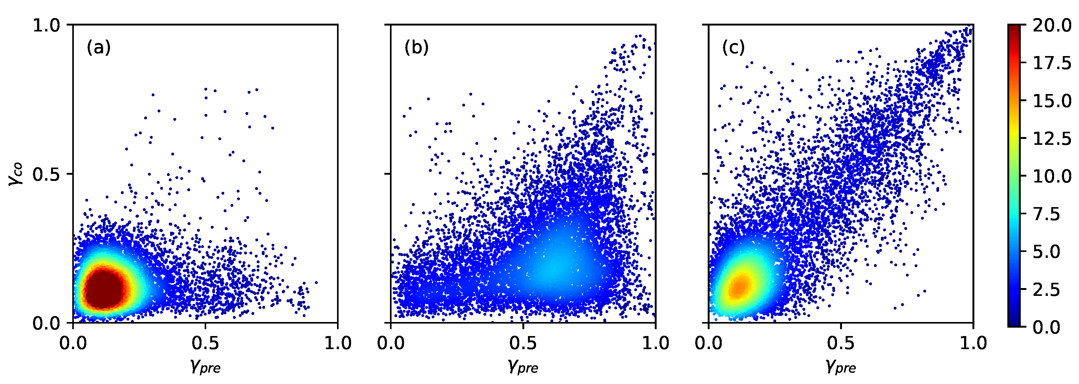
3.3. A New Metric: Conditional Coherence

At this stage, it is clear that traditional methods may cause false detection of flooded areas for agricultural targets. It is imperative to track the periodic activities of agricultural targets and, consequently, be aware of the dynamics of the backscattering sigma naught. Additional information might be useful to judge the reliability of the results. Therefore, for future references, it is strongly recommended to verify whether a flood event occurred during the onset of the irrigation period; if that is not the case, then the previous approaches should be adequate. In case a similar situation occurs, new solutions are required. It is our belief that new solutions should consider the spatial arrangements of the fields and how the waterbodies are present in flooded and non-flooded agricultural targets. A first important fact is that the agricultural fields have a defined shape, which is often rectangular with its edges bounded by street, roads, alleys, or buildings. Another key feature is that the waterbodies in non-flooded fields are stored in a controlled manner; namely, they have the same shape as the agricultural fields (Figure 3). On the other hand, waterbodies in flooded areas do not have a clear defined shape.

The automatic detection of regular shapes, such as rectangular, might be a potential solution to discriminate non-flooded agricultural areas from those that are flooded. There is extensive literature regarding this purpose [26,27,28,29]. Although object detection it is a mature subject, it is worth mentioning the edges of the agricultural fields are not clear defined in microwave images because of the speckle noise; and thus it might not be a straightforward procedure. Current technologies such as supervised machine/deep learning methods can overcome this issue if a proper and extensive training data is at hand and extensive computational resources are available. Instead, we propose a novel heuristic metric, which is based on the fact that the waterbodies in non-flooded paddy fields are stored within the agricultural fields. Thus, the areas between consecutive paddy fields, commonly used for transportation, and all nearby infrastructure remain dry with a more steady backscattering mechanism over time. We then propose to recompute coherence under the following modifications.

Given the X and Y domains, defined as $L_x=\{0,1,\dots ,N_x\}$ and $L_y=\{0,1,\dots ,N_y\}$, respectively, a complex SAR image can be defined as a function that assigns a complex number to each pixel in $L_x\times L_y$; $I:L_x\times L_y\to \mathbb{C}$. Let $A_T$ be a subset of pixel coordinates in $L_x\times L_y$ whose pixel value in the post-event image $I^{pos}$ meets the following condition,

$$A_T=\{(i,j)\in L_x\times L_y|20{log}_{10}|I_{i,j}^{pos}|>T\}$$

(2)

where T is a threshold to filter out pixels with low intensity (units of dB). The coherence between $I^{pos}$ and a pre-event image $I^{pre}$ computed over pixels whose coordinates belong to A is referred to in this paper as “conditional coherence” (${\gamma }_T$):

$${\gamma }_T=\frac{|{\sum }_{(i,j)\in A_T}{I}_{i,j}^{pre}{I_{i,j}^{pos}}^{\ast }|}{\sqrt{{\sum }_{(i,j)\in A_T}{I}_{i,j}^{pre}{I_{i,j}^{pre}}^{\ast }{\sum }_{(i,j)\in A_T}{I}_{i,j}^{pos}{I_{i,j}^{pos}}^{\ast }}}$$

(3)

The concept behind Equation (3) is to recompute the coherence after filtering low-intensity pixels at the post-event SAR image using a user-defined threshold, T. A suitable option for T is the same threshold used to create waterbodies map in Figure 2b. The low intensity pixels are filtered out because these are the information the flooded and non-flooded agricultural targets have in common. On the other hand, medium/large intensity pixels do have different pattern. For the purpose of identifying flooded areas in agricultural targets, the conditional coherence must be computed over a moving window which size (i.e., $N_x$ and $N_y$) should be large enough to include paddy field edges and surrounding structures.

3.4. Machine Learning Classification

The performance of the conditional coherence as input of a machine learning classifiers to characterize flooded and non-flooded agricultural fields is evaluated here. Two different machine learning classifiers that can be used in different circumstances are evaluated. In a first situation, it is assumed that there is not information other than the remote sensing data. That is, there is no available truth data. Then, under this context, an unsupervised machine learning classifier is a suitable option. In a second circumstance, areas confirmed as flooded at a very early stage of the disaster are used as input of a supervised machine learning classification.

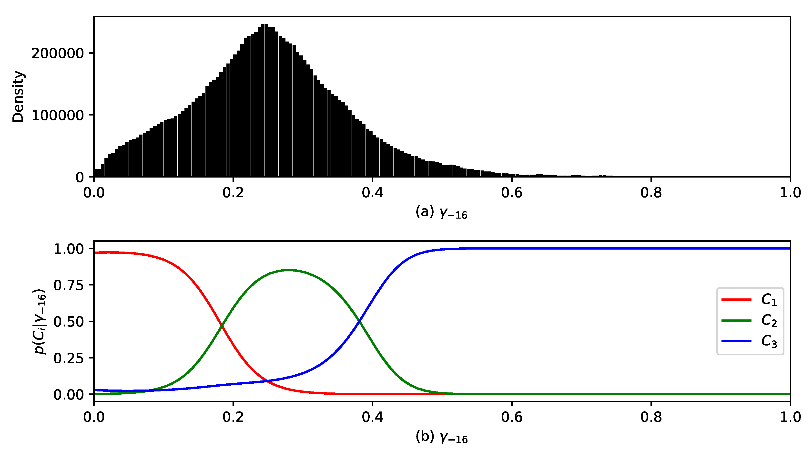
3.4.1. Unsupervised Classification

The expectation–maximization (EM) algorithm [30,31], an unsupervised classifier, is here used to discriminate the flooded and non-flooded agricultural targets. The EM algorithm considers that the distribution of the conditional coherence is composed of a mixture of distributions:

$$p({\gamma }_T)=\sum _{i=1}^{k}p({\gamma }_T|C_i)P(C_i)$$

(4)

where k is the number of classes defined beforehand, $C_i$ denotes a class, and $P(C_i)$ are the mixture proportions. The distributions are defined from an iterative optimization. For instance assuming Gaussian distributions, the calibration of their parameters is as follows,

$$\begin{array}{cc}\hfill & {\mu }_i^{l+1}=\frac{{\sum }_t{h}_i^t{\gamma }_{T_i}^t}{{\sum }_t{h}_i^t}\hfill \\ \hfill & S_i^{l+1}=\frac{{\sum }_t{h}_i^t{({\gamma }_{T_i}^t-m_i^{l+1})}^2}{{\sum }_t{h}_i^t}\hfill \\ \hfill & h_i^t=\frac{P(C_i){\left|S_i\right|}^{-1/2}exp\left(-1/2{({\gamma }_{T_i}^t-m_i)}^2{S}_i^{-1}\right)}{{\sum }_{j}P(C_j){\left|S_j\right|}^{-1/2}exp\left(-1/2{({\gamma }_{T_i}^t-m_j)}^2{S}_j^{-1}\right)}\hfill \end{array}$$

(5)

where $m_i$ and $S_i$ denote the vector mean and variance, respectively. In this study, Gaussian distributions are used. After a calibration of the distributions through the iterative process, each pixel sample is associated with the class $C_i$ that gives the maximum $p({\gamma }_T|C_i)$.

3.4.2. Supervised Thresholding

Areas recognized as flooded immediately after the floods occurred are used here to define a range in ${\gamma }_{-16}$ and use it to perform predictions. Namely, new samples that are located inside the range will be classified as flooded; otherwise, it will be classified as non-flooded. The decision whether a sample belong to a flooded sample is based on the sign of the following expression:,

$$f({\gamma }_T)=w·{\gamma }_T+\rho$$

(6)

where the parameters w and $\rho$ are calculated from the following optimization problem,

$$\begin{array}{cc}\hfill & \underset{w,\rho }{min}\frac{1}{2}{w}^2+\frac{1}{vl}\sum _i{\xi }_i-\rho \hfill \\ \hfill & \mathrm{subject}\mathrm{to}w·{\gamma }_{T_i}\ge \rho -{\xi }_i,{\xi }_i>0\hfill \end{array}$$

(7)

where ${\gamma }_{T_i}$ is the conditional coherence of sample $i\in \{1,\dots ,N\}$, with N being the number of samples; ${\xi }_i$ is a slack variable; and $\nu \in (0,1]$ denotes the upper bound of the fraction of outlier samples. Equations (6) and (7) denote a particular case of the method proposed by Schölkopf et al. [32], from which the case of multidimensional features is tamed.

4. Results

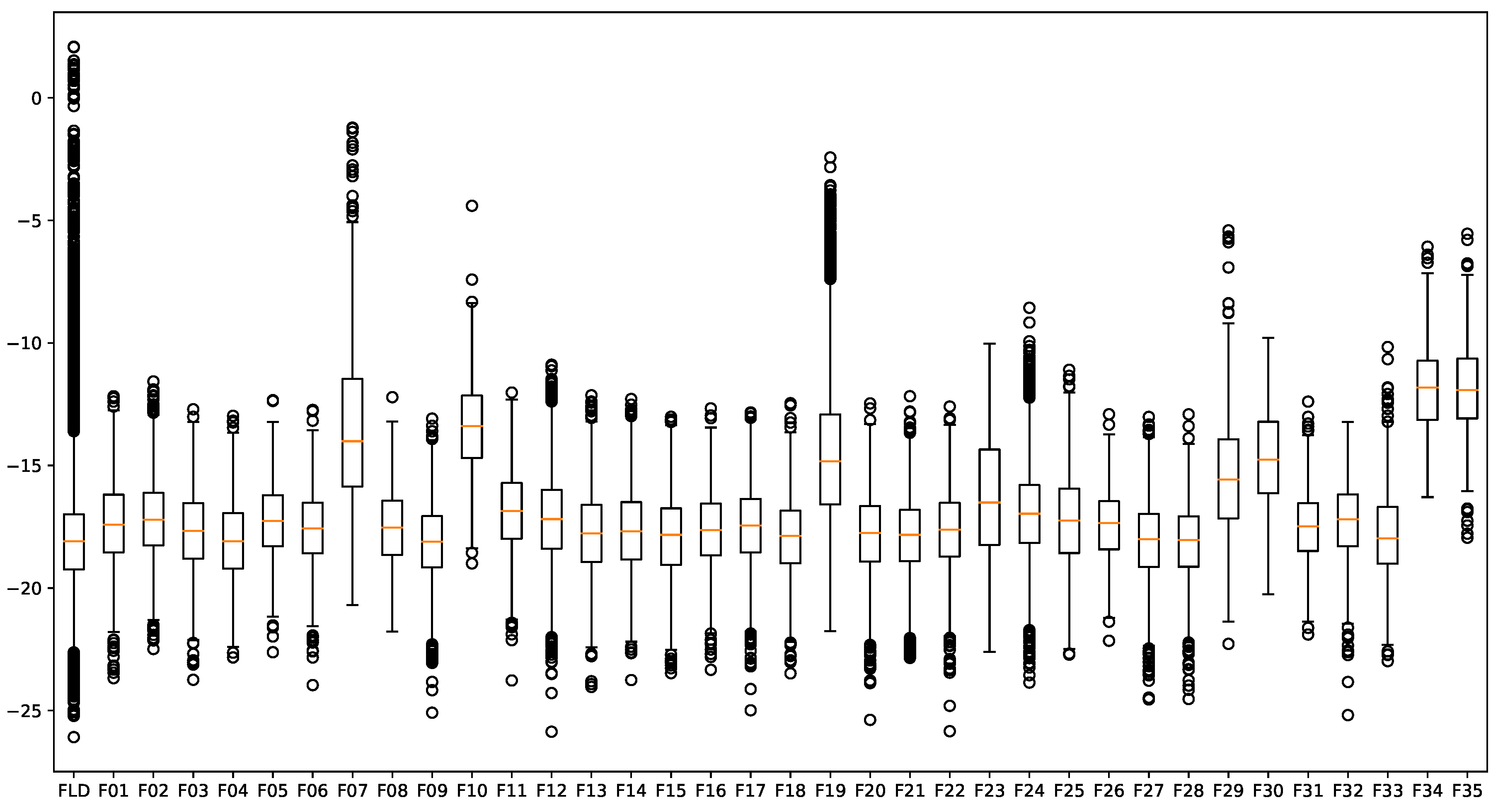
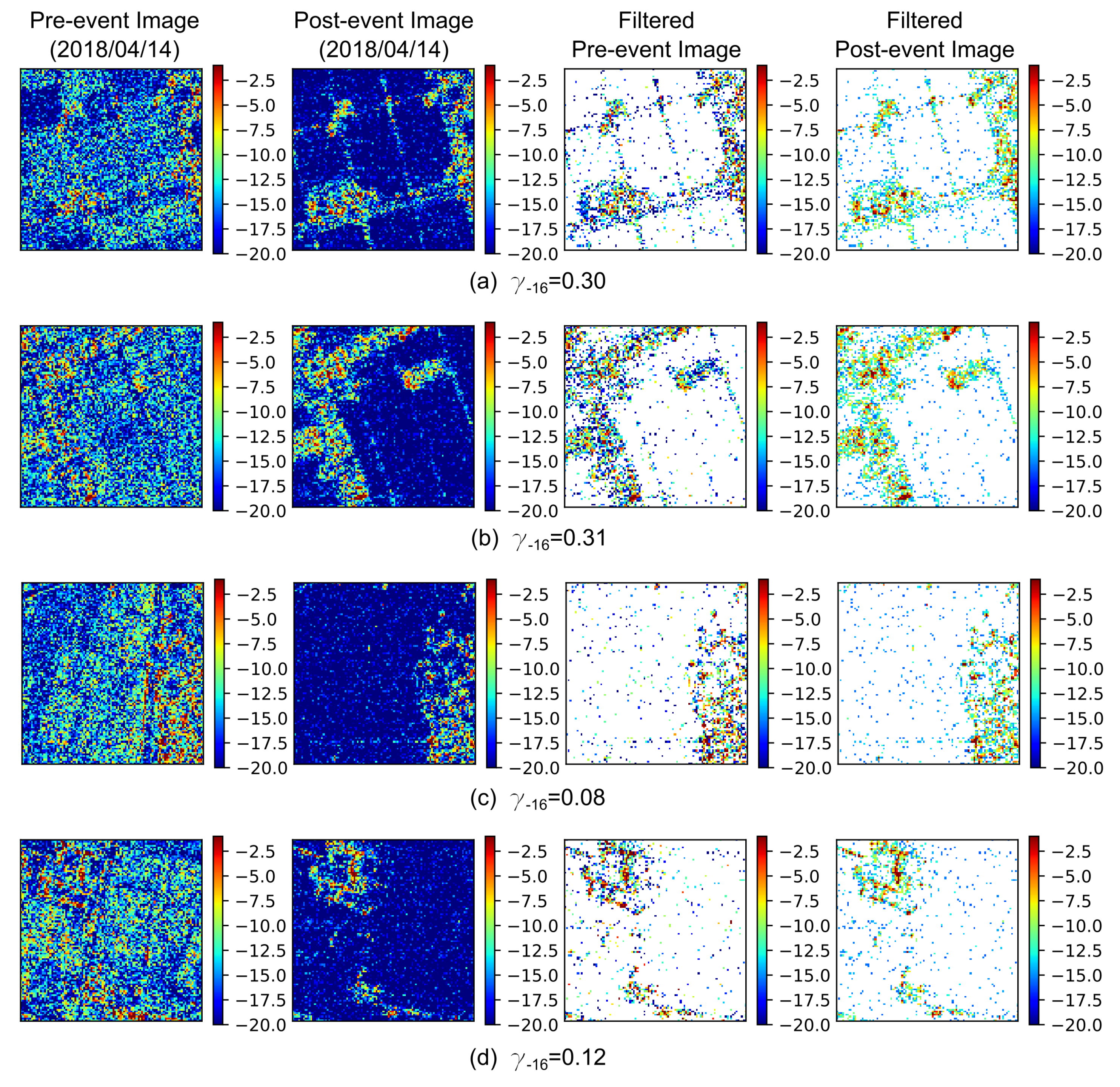
4.1. Conditional Coherence

Figure 8a,b shows subimages of $101\times 101$ pixels of two non-flooded agricultural targets located within the NF-area. Both, the pre-event and post-event SAR images are depicted. After removing pixels whose intensity at the post-event image was lower than −16 dB (i.e., pixels whose coordinates do not belong to $A_{-16}$), the remaining pixels consist of those located in the paths between paddy fields and/or the infrastructure nearby. The conditional coherence computed at both pairs of images is ~0.30. Likewise, Figure 8c,d shows subimages of flooded agricultural targets located within the F-area. Note that, unlike the non-flooded agriculture areas, the street/roads between consecutive fields are not visible in the post-event subimages. In Figure 8c, the area with high backscattering intensity at the bottom-right consists of a flooded urban area. The conditional coherence computed in this subimage is ${\gamma }_{-16}=0.08$. The high value pixels at the top left of Figure 8d represent the backscattering intensity from the Prefectural School of Okayama Kurashikimakibishien, which was inundated as well. The conditional coherence at this area is ${\gamma }_{-16}=0.12$. Note that, although in the four examples the conditional coherence is rather low, those computed in flooded areas are lower than those computed in non-flooded areas. Within flooded areas, large intensity pixels are mainly due to the join effect of specular-reflection and double-bouncing backscattering mechanisms; whereas in non-flooded areas, the medium/large intensity pixels denotes the backscattering from the street/roads and nearby buildings.

Figure 9 illustrates ${\gamma }_{-16}$ computed over the waterbodies shown in Figure 2b. A window size of $101\times 101$ pixels (approximately $300\times 300{\mathrm{m}}^2$) was used. Recall that Figure 2b depicts the areas with the lowest backscattering intensity, and thus the conditional coherence at each pixel in Figure 9 contains information of its surroundings rather than its location. It is observed that in both the flooded and non-flooded areas, the conditional coherence is mostly lower than 0.5. However, it is clearly observed that the conditional coherence in Mabi-town is much lower than that computed in the surveyed paddy fields. Figure 10 top shows the distribution of ${\gamma }_{-16}$. The distribution is slightly skewed to the right, which is the effect of the low conditional coherence at the flooded agricultural areas. It does not exhibit a bimodal distribution, with a distinctive peak representing the flooded agricultural targets, because the population of non-flooded areas is much larger than that from the flooded areas. Furthermore, although difficult to observe, there are several thousands of samples with ${\gamma }_{-16}$ greater than 0.5.

4.2. Classification of Flooded and Non-Flooded Agriculture Targets

Considering the shape of the distribution of ${\gamma }_{-16}$ (Figure 10a), the EM algorithm was computed for three classes ($k=3$). Then, the class that contains the lowest ${\gamma }_{-16}$ is considered a flooded area, and the other two classes are merged to represent the non-flooded areas. Figure 10b shows the $p(C_i|{\gamma }_{-16})$ for the three classes and Figure 11a shows the resulted classification map. The red pixels denote the flooded agricultural areas, whereas the blue ones denote the non-flooded agricultural areas. Figure 11b shows a closer look of the flooded paddy fields at the F-area. It is observed that the resulting classification using the conditional coherence is consistent with the area delineated by GSI. Figure 11c shows a closer look of the NF-area. Compared with Figure 2b, it is observed that most of the false detection has been rectified. However, in the bottom right of Figure 11c, it is observed an area classified as flooded paddy field. Figure 9 shows that indeed the area exhibit low conditional coherence. A closer look revealed there was a significant amount of dry vegetation at a higher elevation than the paddy fields, which certainly will exhibit medium backscattering intensity, but low coherence and conditional coherence.

Regarding the classification using the one-class SVM method, 30,000 samples of flooded agricultural targets were randomly extracted from the green polygons denoted in Figure 5b. Note the referred area was promptly confirmed as flooded, and it is located within the F-area. The parameter $\nu$ of the Equation (7) was chosen to be 0.95. That is, the calibrated function can accept a maximum of 5% of outliers from the input samples. Figure 12a shows the distribution of the input samples with respect to ${\gamma }_{-16}$. Figure 12b shows the calibrated $f({\gamma }_{-16})$. As mentioned previously, the value in which $f({\gamma }_{-16})$ changes sign is the boundary between the two classes. Such value is slightly lower than 0.2. Therefore, a lower value is classified as flooded agriculture area; otherwise, it is classified as non-flooded agricultural area. Note, the boundary between the two classes are practically the same as the one defined with the EM method, and therefore the map of flooded and non-flooded agricultural targets computed from the one-class SVM method (Figure 13) is very similar to that computed from the EM algorithm (Figure 11).

To evaluate the performance of the classifiers calibrated using the EM and the one-class SVM methods, pixels within the area delineated by GSI at Mabi town and pixels within the NF-area are used as reference pixels of flooded and non-flooded agriculture areas. A proper evaluation requires the same amount of samples for each class. Thus, 10,000 pixels are extracted randomly from each of the referred areas. Three scores are used for the evaluation: producer accuracy (PA), user accuracy (UA), and F1. The PA represents the percentage of samples extracted from the GSI-area (NF-area) that were classified as flooded (non-flooded). Similarly, the UA is the percentage of samples classified as flooded (non-flooded) that were extracted from the GSI-area (NF-area). The F1 is computed from the following expression, $2{(U{A}^{-1}+P{A}^{-1})}^{-1}$. To consider the effect of the random sampling, the evaluation was performed a hundred times. Figure 14 reports the resulting scores. It is observed all the scores have the value of ~81%, which indicates high accuracy.

Table 1. Prediction of flooded and non-flooded areas at the areas depicted by GSI, the field survey at the agricultural targets, and the NF-area.

	EM		One-Class SVM		Total
	Flooded	Non-Flooded	Flooded	Non-Flooded
GSI	327,464	60,012	327,306	65,170	392,476
Survey	319	28,476	308	28,487	28,795
NF-area	813,561	3,069,984	810,299	3,073,246	3,883,545

reports the predictions over the all pixels in the GSI-area, the surveyed paddy fields, and the NF-area.

5. Discussion

Additional comments regarding the relevance of this study are necessary. In the aftermath of the 2018 Western Japan floods, preliminary estimations of the affected areas were published. As this study proved, all flood maps estimated from the L-band SAR images overestimated the floods in Okayama Prefecture. Such significant overestimation can compromise an efficient transfer of human and material resources. It was, therefore, of great interest the identification of the factors that induced such misclassifications. This study showed that the main factors are the use of only two images, the L-band wavelength, and the onset of agricultural activities. Another factor that may have influenced the large misclassifications is the use of automatic procedures without human intervention. We belief that such an importance task should be supervised by an expert to make a proper interpretation of the microwave imagery and the resulted flood map. For the main role of an automatic procedure is to assist the experts on getting a fast estimation of the affected area.

Note that the definition of flooded and non-flooded vegetation in [9] differs from ours. In [9], flooded vegetation are vegetation that contain water beneath it; whereas non-flooded vegetation does not contain water at all. In our study, both flooded and non-flooded agriculture targets contains waterbodies. The water in flooded areas was produced by the flood; whereas non-flooded areas contains water from ordinary irrigation activities. The study of Pierdicca et al. [8] on the potential of CSK to map flooded agricultural fields, see Section 1, did not consider the situation where both the agricultural targets flooded by the natural phenomenon and those artificially flooded for irrigation purposes occur simultaneously.

Regarding the conditional coherence, note that its value contains local information from the field edges and nearby structures; and thus, the window size need to be large enough to include them. As a consequence, the resolution is decreased. Furthermore, note that the window size needs to be defined by the user in advance, which requires rough estimation of the dimensions of a standard agriculture field. The term “conditional” to the conditional coherence is used because a condition was imposed to the pixels used in the computation of the coherence. In this study, the condition was associated to the intensity of the backscattering. Namely, their intensity must be larger than certain threshold. However, other types of conditions can be used to fulfill specific needs.

6. Conclusions

We have reported a case where the change detection approach was not suitable for identifying flooded areas in agricultural targets. It was the co-occurrence of many factors, such as the use of only two images, the L-band wavelength, and the onset of agricultural activities, that produced such misclassifications. Using the backscattering intensity, significant overestimation was produced, and no changes were observed from coherence images. Furthermore, solid evidence from field survey and Sentinel-1 SAR time series data demonstrated that this flaw might occur in future events. We strongly recommend awareness of the dynamics of backscattering in agricultural fields to avoid false alarms. Furthermore, we proposed a new metric, termed here as “conditional coherence”, to infer whether a detected change is associated with non-flooded or flooded agricultural areas. The conditional coherence is a simple modification of the well-known coherence. Thus, its computation is simple, it is computationally efficient, and does not require additional ancillary data (such as optical images and/or land use map). The conditional coherence was computed over the waterbodies observed in flooded and non-flooded agriculture targets, and then, they were used as input feature to perform unsupervised and supervised classifications. Both methods, applied independently, showed the same results; and thus, it confirms that the conditional coherence contains information that can be useful to discriminate flooded agricultural targets. It was observed the resulted classification cleaned up ~81% of the false detection of flooded areas.

References

1. Duan, W.; He, B.; Nover, D.; Fan, J.; Yang, G.; Chen, W.; Meng, H.; Liu, C. Floods and associated socioeconomic damages in China over the last century. Nat. Hazards 2016, 82, 401–413. [Google Scholar] [CrossRef]
2. Morris, J.; Brewin, P. The impact of seasonal flooding on agriculture: the spring 2012 floods in Somerset, England. J. Flood Risk Manag. 2014, 7, 128–140. [Google Scholar] [CrossRef]
3. Schumann, G.J.P.; Moller, D.K. Microwave remote sensing of flood inundation. Phys. Chem. Earth 2015, 83–84, 84–95. [Google Scholar] [CrossRef]
4. Nakmuenwai, P.; Yamazaki, F.; Liu, W. Automated Extraction of Inundated Areas from Multi-Temporal Dual-Polarization RADARSAT-2 Images of the 2011 Central Thailand Flood. Remote Sens. 2017, 9, 78. [Google Scholar] [CrossRef]
5. Liu, W.; Yamazaki, F. Review article: Detection of inundation areas due to the 2015 Kanto and Tohoku torrential rain in Japan based on multitemporal ALOS-2 imagery. Nat. Hazards Earth Syst. Sci. 2018, 18, 1905–1918. [Google Scholar] [CrossRef]
6. Boni, G.; Ferraris, L.; Pulvirenti, L.; Squicciarino, G.; Pierdicca, N.; Candela, L.; Pisani, A.R.; Zoffoli, S.; Onori, R.; Proietti, C.; et al. A Prototype System for Flood Monitoring Based on Flood Forecast Combined With COSMO-SkyMed and Sentinel-1 Data. IEEE J. Sel. Top. Appl. Earth Obs. Remote. Sens. 2016, 9, 2794–2805. [Google Scholar] [CrossRef]
7. Pulvirenti, L.; Chini, M.; Pierdicca, N.; Guerriero, L.; Ferrazzoli, P. Flood monitoring using multitemporal COSMO-SkyMed data: Image segmentation and signature interpretation. Remote Sens. Environ. 2011, 115, 990–1002. [Google Scholar] [CrossRef]
8. Pierdicca, N.; Pulvirenti, L.; Boni, G.; Squicciarino, G.; Chini, M. Mapping Flooded Vegetation Using COSMO-SkyMed: Comparison With Polarimetric and Optical Data Over Rice Fields. IEEE J. Sel. Top. Appl. Earth Obs. Remote. Sens. 2017, 10, 2650–2662. [Google Scholar] [CrossRef]
9. Pulvirenti, L.; Pierdicca, N.; Chini, M.; Guerriero, L. Monitoring Flood Evolution in Vegetated Areas Using COSMO-SkyMed Data: The Tuscany 2009 Case Study. IEEE J. Sel. Top. Appl. Earth Obs. Remote. Sens. 2013, 6, 1807–1816. [Google Scholar] [CrossRef]
10. Sui, H.; An, K.; Xu, C.; Liu, J.; Feng, W. Flood Detection in PolSAR Images Based on Level Set Method Considering Prior Geoinformation. IEEE Geosci. Remote Sens. Lett. 2018, 15, 699–703. [Google Scholar] [CrossRef]
11. Arnesen, A.S.; Silva, T.S.; Hess, L.L.; Novo, E.M.; Rudorff, C.M.; Chapman, B.D.; McDonald, K.C. Monitoring flood extent in the lower Amazon River floodplain using ALOS/PALSAR ScanSAR images. Remote Sens. Environ. 2013, 130, 51–61. [Google Scholar] [CrossRef]
12. Moya, L.; Marval Perez, L.R.; Mas, E.; Adriano, B.; Koshimura, S.; Yamazaki, F. Novel Unsupervised Classification of Collapsed Buildings Using Satellite Imagery, Hazard Scenarios and Fragility Functions. Remote Sens. 2018, 10, 296. [Google Scholar] [CrossRef]
13. Moya, L.; Yamazaki, F.; Liu, W.; Yamada, M. Detection of collapsed buildings from lidar data due to the 2016 Kumamoto earthquake in Japan. Nat. Hazards Earth Syst. Sci. 2018, 18, 65–78. [Google Scholar] [CrossRef] [Green Version]
14. Moya, L.; Mas, E.; Adriano, B.; Koshimura, S.; Yamazaki, F.; Liu, W. An integrated method to extract collapsed buildings from satellite imagery, hazard distribution and fragility curves. Int. J. Disaster Risk Reduct. 2018, 31, 1374–1384. [Google Scholar] [CrossRef]
15. Moya, L.; Zakeri, H.; Yamazaki, F.; Liu, W.; Mas, E.; Koshimura, S. 3D gray level co-occurrence matrix and its application to identifying collapsed buildings. ISPRS J. Photogramm. Remote. Sens. 2019, 149, 14–28. [Google Scholar] [CrossRef]
16. Endo, Y.; Adriano, B.; Mas, E.; Koshimura, S. New Insights into Multiclass Damage Classification of Tsunami-Induced Building Damage from SAR Images. Remote Sens. 2018, 10, 2059. [Google Scholar] [CrossRef]
17. Adriano, B.; Xia, J.; Baier, G.; Yokoya, N.; Koshimura, S. Multi-Source Data Fusion Based on Ensemble Learning for Rapid Building Damage Mapping during the 2018 Sulawesi Earthquake and Tsunami in Palu, Indonesia. Remote Sens. 2019, 11, 886. [Google Scholar] [CrossRef]
18. Karimzadeh, S.; Mastuoka, M. Building Damage Assessment Using Multisensor Dual-Polarized Synthetic Aperture Radar Data for the 2016 M 6.2 Amatrice Earthquake, Italy. Remote Sens. 2017, 9, 330. [Google Scholar] [CrossRef]
19. Rosenqvist, A. Temporal and spatial characteristics of irrigated rice in JERS-1 L-band SAR data. Int. J. Remote Sens. 1999, 20, 1567–1587. [Google Scholar] [CrossRef]
20. Le Toan, T.; Laur, H.; Mougin, E.; Lopes, A. Multitemporal and dual-polarization observations of agricultural vegetation covers by X-band SAR images. IEEE Trans. Geosci. Remote Sens. 1989, 27, 709–718. [Google Scholar] [CrossRef]
21. Kurosu, T.; Fujita, M.; Chiba, K. Monitoring of rice crop growth from space using the ERS-1 C-band SAR. IEEE Trans. Geosci. Remote Sens. 1995, 33, 1092–1096. [Google Scholar] [CrossRef]
22. Cabinet Office of Japan. Summary of Damage Situation Caused by the Heavy Rainfall in July 2018. Available online: http://www.bousai.go.jp/updates/h30typhoon7/index.html (accessed on 7 August 2018).
23. Plank, S. Rapid damage assessment by means of multitemporal SAR—A comprehensive review and outlook to Sentinel-1. Remote Sens. 2014, 6, 4870–4906. [Google Scholar] [CrossRef]
24. Geospatial Information Authority of Japan. Information about the July 2017 Heavy Rain. Available online: https://www.gsi.go.jp/BOUSAI/H30.taihuu7gou.html (accessed on 19 July 2019).
25. The International Charter Space and Major Disasters. Flood in Japan. Available online: https://disasterscharter.org/en/web/guest/activations/-/article/flood-in-japan-activation-577- (accessed on 22 January 2019).
26. Wang, Z.; Ben-Arie, J. Detection and segmentation of generic shapes based on affine modeling of energy in eigenspace. IEEE Trans. Image Process. 2001, 10, 1621–1629. [Google Scholar] [CrossRef] [PubMed]
27. Moon, H.; Chellappa, R.; Rosenfeld, A. Optimal edge-based shape detection. IEEE Trans. Image Process. 2002, 11, 1209–1227. [Google Scholar] [CrossRef] [PubMed]
28. Wang, J.; Athitsos, V.; Sclaroff, S.; Betke, M. Detecting Objects of Variable Shape Structure With Hidden State Shape Models. IEEE Trans. Pattern Anal. Mach. Intell. 2008, 30, 477–492. [Google Scholar] [CrossRef] [PubMed]
29. Li, Q. A Geometric Framework for Rectangular Shape Detection. IEEE Trans. Image Process. 2014, 23, 4139–4149. [Google Scholar] [CrossRef] [PubMed]
30. Dempster, A.P.; Laird, N.M.; Rubin, D.B. Maximum likelihood from incomplete data via the EM algorithm. J. R. Statist. Soc. B 1977, 39, 1–38. [Google Scholar] [CrossRef]
31. Redner, R.A.; Walker, H.F. Mixture Densities, Maximum Likelihood and the Em Algorithm. SIAM Rev. 1984, 26, 195–239. [Google Scholar] [CrossRef]
32. Schölkopf, B.; Platt, J.C.; Shawe-Taylor, J.C.; Smola, A.J.; Williamson, R.C. Estimating the Support of a High-Dimensional Distribution. Neural Comput. 2001, 13, 1443–1471. [Google Scholar] [CrossRef]
Figure 1. Geographical location of the study area. The polygons at Mabi town denotes the estimated flooded area provided by Geospatial Information Authority of Japan (GSI). The polygons labeled as surveyed area denotes the paddy fields that were inspected.
Remotesensing 11 02320 g001
Figure 2. (a) Color composite of pre- and post-event ALOS-2 SAR images. The inset denotes the location of the study area in the western Japan. (b) Thresholding-based water body identification. The black rectangles denote confirmed flooded and non-flooded agriculture areas.
Remotesensing 11 02320 g002
Figure 3. (a): Surveyed paddy fields (red rectangles) located within the NF-area shown in Figure 2. (b,c): Survey photos of paddy fields.
Remotesensing 11 02320 g003
Figure 4. Boxplot of blackscatteringsigma naught of the flooded (FLD) and non-flooded paddy field (F01–F35) areas.
Remotesensing 11 02320 g004
Figure 5. RGB color composite of co-event (R) and pre-event (G and B) coherence images. (a) Study area. (b) Closer look of Mabi-town (yellow rectangle in panel a). Red and green dashed polygons indicate instances of flooded urban and agricultural areas, respectively.
Remotesensing 11 02320 g005
Figure 6. Pre-event ( γ p r e ) and co-event ( γ c o ) coherence scatter plots computed for (a) flooded agricultural areas, (b) flooded urban areas, and (c) non-flooded agricultural areas. Color marks denote the frequency of occurrence. Each plot consists of 10,000 samples extracted randomly from the polygons depicted in Figure 5b and the surveyed paddy fields (Figure 3a).
Remotesensing 11 02320 g006
Figure 7. Temporal variation in backscattering from surveyed paddy field F26. The red and blue lines denote the mean variations during the years 2017 and 2018, respectively. The shaded area denotes the limits of the average plus/minus one standard deviation. The vertical dashed lines denote the date of the field survey (25 July 2018) and the dates of the ALOS-2 SAR images that were provided for the early response.
Remotesensing 11 02320 g007
Figure 8. Examples of conditional coherence computed with T = 16 ( γ 16 ). The two leftmost columns depict the pre-event and post-event SAR backscattering intensity. The two rightmost columns show only the pixels whose location belongs to the subset A 16 . (a,b) Examples of non-flooded agriculture targets. (c,d) Examples of flooded agriculture targets.
Remotesensing 11 02320 g008
Figure 9. Conditional coherence γ 16 computed over the waterbodies identified in Figure 2.
Remotesensing 11 02320 g009
Figure 10. (a) Distribution of γ 16 shown in Figure 9. (b) The conditional probabilities that a sample belongs to class C 1 (red line), C 2 (blue line), and C 3 (green line) resulted from the EM algorithm.
Remotesensing 11 02320 g010
Figure 11. (a) EM classification of flooded (red pixels) and non-flooded (cyan pixels) agricultural targets. (b) Closer look of the F-area. The black polygons represent the flooded area provided by GSI. (c) Closer look at the NF-area.
Remotesensing 11 02320 g011
Figure 12. (a) Distribution of γ 16 computed over pixels located in the green polygon at Figure 5b. (b) Discriminant function (Equation (6)) calibrated from the one-class SVM method.
Remotesensing 11 02320 g012
Figure 13. (a) One-class SVM classification of flooded (red pixels) and non-flooded (cyan pixels) agricultural targets. (b) Closer look of the F-area. The black polygons represent the flooded area provided by GSI. (c) Closer look at the NF-area.
Remotesensing 11 02320 g013
Figure 14. Producer accuracy (red lines), user accuracy (green lines), and F1 (blue lines) scores for flooded (solid lines) and non-flooded (dashed lines) agricultural targets. (a) Scores computed from the classification of the EM algorithm. (b) Scores computed from the classification of the one-class SVM.
Remotesensing 11 02320 g014