Article

Weighted Double-Logistic Function Fitting Method for Reconstructing the High-Quality Sentinel-2 NDVI Time Series Data Set

1
Aerospace Information Research Institute, Chinese Academy of Sciences, Beijing 100101, China
2
University of Chinese Academy of Sciences, Beijing 100049, China
3
Agricultural Science and Technology Information Research Institute, Guangxi Academy of Agricultural Sciences, Nanning 530007, China
4
College of Computer Science and Technology, Zhejiang University of Technology, Hangzhou 310014, China
*
Author to whom correspondence should be addressed.
Remote Sens. 2019, 11(20), 2342; https://doi.org/10.3390/rs11202342
Submission received: 22 August 2019 / Revised: 6 October 2019 / Accepted: 8 October 2019 / Published: 9 October 2019
(This article belongs to the Section Remote Sensing Image Processing)

Abstract

:
The time series (TS) of the normalized difference vegetation index (NDVI) has been widely used to trace the temporal and spatial variability of terrestrial vegetation. However, many factors such as atmospheric noise and radiometric correction residuals conceal the actual variation in the land surface, and thus hamper the TS information extraction. To minimize the negative effects of these noise factors, we propose a new method to produce a synthetic gap-free NDVI TS from the original contaminated observation. First, the key temporal points are identified from the NDVI time profiles based on a generally used rule-based strategy, making the TS segmented into several adjacent segments. Then, the observed data points in each segment are fitted with a weighted double-logistic function. The proposed dynamic weight reassignment process effectively emphasizes cloud-free points and deemphasizes cloud-contaminated points. Finally, the proposed method is evaluated on more than 3,000 test points from three selected Sentinel-2 tiles, and is compared with the generally used Savitzky-Golay (S-G) and harmonic analysis of time series (HANTS) methods from qualitative and quantitative aspects. The results indicate that the proposed method has a higher capability of retaining cloud-free data points and identifying outliers than the others, and can generate a gap-free NDVI time profile derived from a medium-resolution satellite sensor.

Graphical Abstract

1. Introduction

The normalized difference vegetation index (NDVI) plays an important role in monitoring dynamic changes in the land surface. The NDVI is calculated from near-infrared radiation scattered by foliage, and red radiation absorbed by chlorophyll. It has been widely accepted in vegetation activity monitoring [1,2,3] since the greenness of vegetation leads to higher NDVI values, and the senescence of vegetation tends to make the NDVI lower. The time series (TS) of the NDVI has been widely applied in monitoring vegetation phenology [4,5,6,7], such as the timing of growth, the timing of senescence and the duration of growth development. The NDVI TS has also been used in land cover mapping [8,9,10,11,12,13] and terrestrial biophysical parameter derivation [14,15]. However, the NDVI values, which are derived from satellite imagery, are affected by cloud contamination, illumination intensity, and sun-target-sensor geometry, making the TS present irregular curves with noise, and therefore the NDVI cannot describe the actual vegetation activity accurately [16].
Atmospheric conditions have great effects on the NDVI products [16,17], for the reason that atmospheric molecular scattering tends to increase red radiation received by the satellite, and red light is more easily scattered by atmospheric particles than near infrared light. This results in the effect of top-of-atmosphere (TOA) NDVI reduction, and hampers the acquisition of vegetation information beneath the clouds.
Therefore, many studies have been devoted to noise reduction in the contaminated NDVI TS, and have reconstructed time series with higher quality [18,19]. Previous analyses on the NDVI have been based on the Advanced Very High Resolution Radiometer (AVHRR) and Moderate Resolution Imaging Spectroradiometer (MODIS) data sources, since the satellites with short revisit cycles can produce daily observations. The commonly used maximum value composite (MVC) [20] method selects the maximum NDVI over a time period to represent the NDVI of the period. This technique can partially alleviate cloud interference and solve the problem of cloud contamination. However, it requires at least one cloud-free observation, and the method may sacrifice short-term variations as well. These problems limit its application to NDVI TS derived from medium-resolution sensors, the revisit frequency of which is a few days. To overcome these problems, more well-designed methods have been developed to reconstruct high-quality NDVI TS. These methods can be categorized into three types: Local filtering methods, function fitting methods and harmonic analysis methods [17,21].
The local filtering methods filter the irregular NDVI TS with a moving window, such as the best index slope extraction (BISE) [22], the modified BISE [23], the mean value iteration (MVI) filter [24], the Savitzky-Golay (S-G) method [17,25] and the changing weight filter (CWF) [21]. These methods can help the filtered TS maintain their original shapes and not greatly deviate from the observed TS. The BISE and MVI techniques rely on a previously set threshold to identify the abnormal points to smooth the NDVI TS. The S-G method is achieved by fitting successive subsets of points into the filter window using a low-degree polynomial with the least squares. The S-G method requires two parameters to be previously set: The polynomial degree and the sliding window size. However, in these methods, the manually-defined thresholds and parameters tend to make the filtering effects unstable and subjective. In addition, they require that the NDVI TS have equal temporal intervals.
Popular function fitting methods include the asymmetric Gaussian (AG) fitting method [26], the double-logistic (DL) function fitting method [27,28] and the high-order annual spline method [29]. Generally, these methods can make the filtered TS smooth. These methods have the advantage of simplicity and flexibility, since the NDVI TS can be expressed with a few coefficients. Most cases can be implemented by minimizing the least squares between the original observed data and the estimates.
Harmonic analysis methods, such as the discrete Fourier transform (DFT) method [30], the harmonic analysis of time series (HANTS) method [31] and the moving weighted harmonic analysis method [21], model the observation TS by using a series of sines and cosines. These methods are based on the idea that phenology has strong seasonality. The harmonic analysis method has been applied in vegetation type classification and coverage estimation based on the shape similarity of the annual NDVI cycles [32]. However, it is not applicable for irregular curves with asymmetric shapes.
In general, NDVI time profiles show different shapes and tendencies because of the various phenological characteristics of vegetation. The periodic activities are different for various vegetation types, and are influenced by seasonal and inter-annual variations in climate. For instance, evergreen forests maintain their foliage during winter, but deciduous forests show stronger seasonal phenology, such as leaf emergence and defoliation. Crop phenology presents high diversity due to climatic factors, such as temperature and precipitation, in different regions. In temperate and tropical zones, crops may have two growth cycles in one year owing to suitable climatic conditions, whereas crops can only grow once in cold regions. Considering the variety of NDVI time profiles, we intend to apply flexible function fitting methods, among which the DL function has been widely applied, to generate high-quality NDVI TS.
The use of the logistic function to fit the time profile of the vegetation index can be traced back to 1980 [33]. According to Fisher [27], the NDVI rises exponentially from the beginning of leaf emergence; after that, when the leaf area index (LAI) increases to some extent, and the lower layer in the canopy can only receive limited radiation, the NDVI is almost linearly related to the absorbed photosynthetically active radiation (PAR). With the senescence (aging) of green vegetation, the leaves become yellow, and the photosynthetic activity terminates, as presented by decreasing NDVI values. Fischer [34] developed a semi-empirical model, named the DL function, with five parameters to represent the annual NDVI time profile, and successfully applied it to homogeneous and heterogeneous croplands. Zhang [28] used the rate of change in curvature based on the DL function to monitor phenology and derive transition dates, namely, the green-up, maturity, senescence and dormancy dates. Beck et al. [2] applied the DL function in monitoring vegetation dynamics at very high latitudes, and the results showed that the DL function outperformed the Fourier series and the asymmetric Gaussian function in describing NDVI TS. Julien and Sobrino [18] used the DL function to derive global land-surface phenology trends from the GIMMS database. These studies have proven the effectiveness and practicability of the DL function in filtering NDVI TS.
However, the abovementioned studies are based on coarse-resolution AVHRR and MODIS composite datasets, which form intensive observations, and are likely to be cloud-free. Currently, medium-resolution datasets from satellites such as Sentinel-2 and Landsat, which revisit the same place for a few days, are commonly used in land-surface monitoring. Directly captured, disturbed information hinders the observation of vegetation. Hence, it results in higher demands for data preprocessing and cloud filtering. In this study, we develop a weighted double-logistic function (WDL) fitting method to reconstruct high-quality NDVI TS. First, we identify key temporal points from the observed data points, which can segment global NDVI TS into several adjacent parts. Then we use the WDL function to fit the data points of a local segment. In the procedure, the importance of cloud-free data is enhanced, while the weights of contaminated data are lowered. The strategy can handle the problem of contaminated data points when adequate multi-observation cloud-free data are lacking.

2. Materials and Methods

2.1. Data Set

Sentinel-2 is an Earth observation mission developed by the European Space Agency (ESA) to execute terrestrial monitoring. The Sentinel-2A satellite was launched on 23 June 2015, followed by the Sentinel-2B satellite on 7 March 2017. The Sentinel-2 mission has the capabilities of 13 multispectral bands (covering visual, near infrared and shortwave infrared spectra), including three red-edge bands, a 10-m spatial resolution in the visible and near infrared bands, a 5-day revisit cycle and a 290-km field of view. The Sentinel-2 mission provides information for agricultural and forestry practices. The satellite data can be used in the Copernicus services, including updating the Coordination of Information on the Environment (CORINE) land cover product. The time series (TS) data set of Sentinel-2 can provide high-frequency observations of the land surface to monitor dynamic changes. Therefore, we use the Sentinel-2 satellite data set to validate the availability of the newly developed method.
We obtained one-year TS of Sentinel-2 Level-1C products (i.e., the top-of-atmosphere (TOA) reflectance products), which were acquired in 2017. Furthermore, the atmospheric correction processor Sen2Cor offered by the ESA was utilized to produce the Level-2A bottom-of-atmosphere (BOA) reflectance products with a 20-m spatial resolution. The Level-2A products also provide the probabilistic cloud mask quality indicator file (CLD), which is derived through a scene classification algorithm. The algorithm is implemented by thresholding band ratios, such as the normalized difference vegetation index (NDVI) and the normalized difference snow index (NDSI), which is calculated from green band (B3) and the shortwave infrared band (B11). It allows detection of clouds, snow and cloud shadows, and generates a classification map, including four different classes for clouds, and six different classifications for shadows, cloud shadows and snow.
For each thresholding test, a level of confidence is associated, which generates a probabilistic cloud mask quality indicator and a snow mask quality indicator. The cloud detection algorithm is implemented by a series of thresholding filtering steps, as shown in Figure 1. In the thresholding algorithm, the final cloud probability is derived step-by-step. The number labeled by ‘*’ means that if the indicator exceeds the threshold, the pixel is considered as cloudy, and the present cloud probability is assigned as 1.0. For instance, ‘B4 > 0.07 (0.25*)’ means when the band 4 reflectance is lower than 0.07, the pixel is considered as cloud-free, and the cloud probability is assigned as 0.0. When this band 4 reflectance is higher than 0.25, the pixel is considered as cloudy, and the cloud probability is assigned as 1.0. When the band 4 reflectance is between 0.07 and 0.25, the pixel is considered as potentially cloudy, and the cloud probability is calculated linearly from 0.0 to 1.0. With the thresholding algorithm proceeding, the present cloud probability is calculated, and then multiplied by a precedent cloud probability which is derived from the previous steps [35]. Accordingly, the CLD can quantitatively show cloud contamination and the level of confidence for the radiometric measurements. Values of 0 and 100 of the CLD indicate the highest and lowest qualities, respectively.
The ESA land cover classification system (LCCS) global land cover product of 2015 was used to select Sentinel-2 test tiles and test points. The pixel size of the land cover product is 300 m.

2.2. Study Area

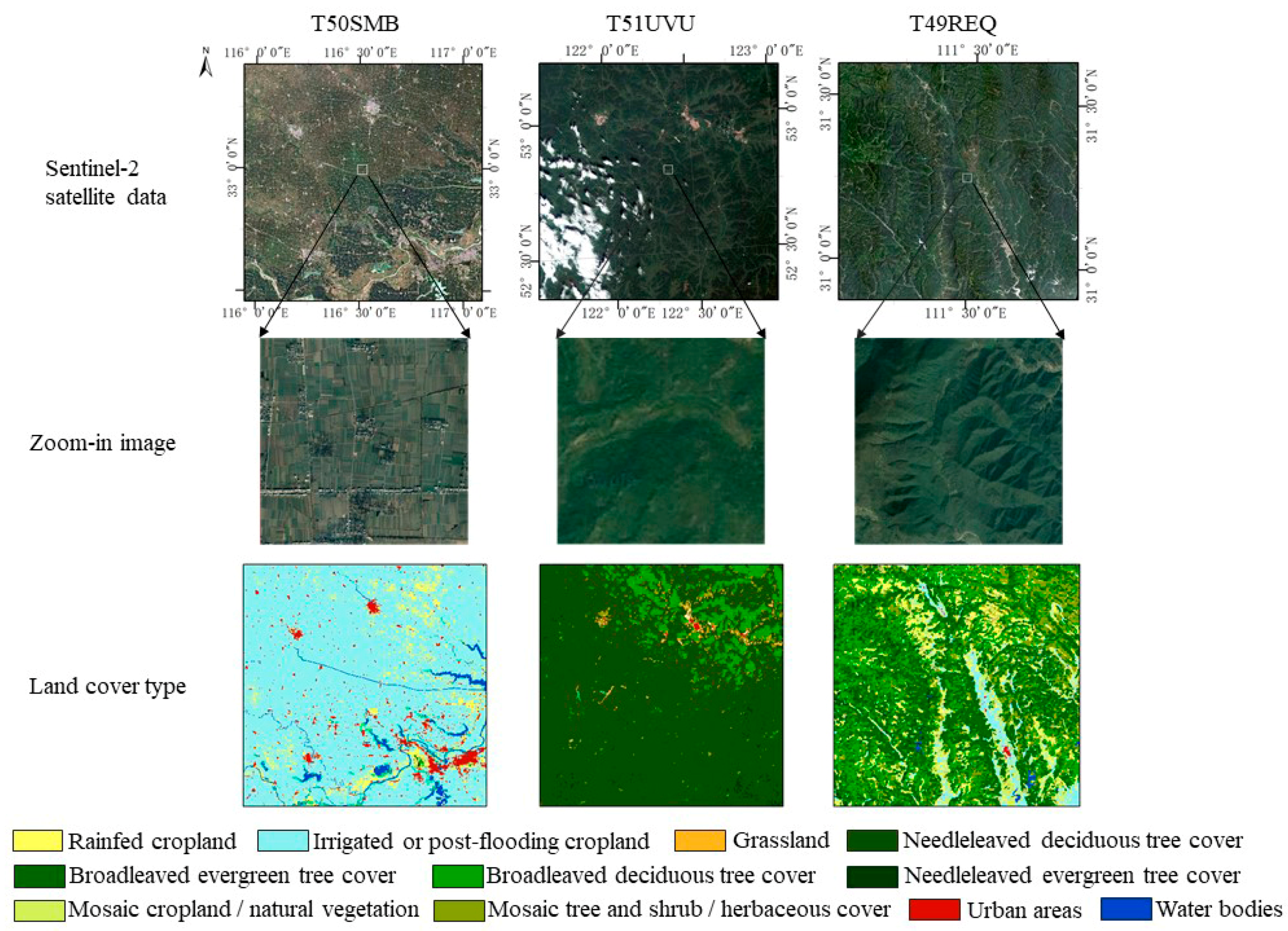
One-year Sentinel-2 TS data set of three study areas (Figure 2) are used to test the proposed technique. The carefully selected tiles cover diverse vegetation types, including coniferous forest, broadleaf forest, grassland and cropland. One study area covered by Sentinel-2 tile T50SMB is located in the south of the Huaiyuan Plain in Anhui Province, China. It is in the transition zone from a subtropical to a warm temperate zone. The moderate temperature and rainfall conditions make the croplands have two growth seasons in one year. The second study area, which is covered by tile T49REQ, is located in Hubei Province, China. It is a mountainous area that is mainly dominated by broadleaved deciduous forests and broadleaved evergreen forests. The third study area is covered by tile T51UVU, mainly located in Heilongjiang Province, China. It belongs to the cold temperate zone, with a continental monsoon climate, and is mainly dominated by deciduous coniferous forests. More than 1,000 test points are randomly generated in each tile, and among them, points classified as vegetation are selected. The sampling point number of the vegetation type for each class in each tile is shown in Table 1.

2.3. Methods

2.3.1. Overview of the proposed method

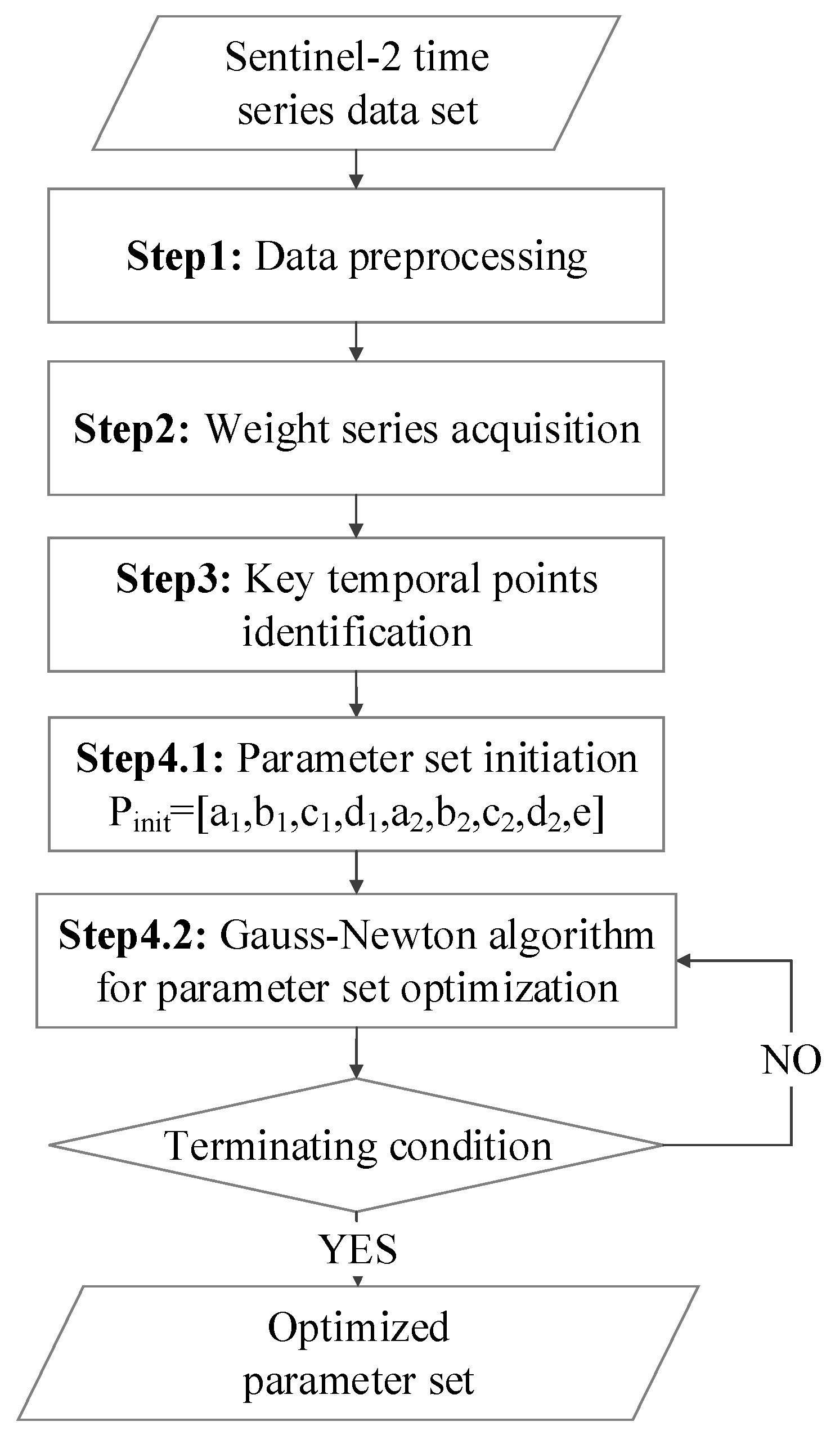
The main steps for the proposed filtering method are shown in the flowchart (Figure 3).

2.3.2. Description of the Proposed Method

1. Data preprocessing
The original NDVI and CLD are temporally organized as follows:
N D V I o r g = [ N D V I 1 , N D V I 2 N D V I k ] ,
C L D o r g = [ C L D 1 , C L D 2 C L D k ]
The data preprocessing procedure is a fundamental and essential step to decrease signal noise. The pixel-level quality flag of the Level-2A product can indicate whether the pixel is atmospherically contaminated, and thus it is preliminarily applied to mark outliers among TS data points. According to experience knowledge, data points with CLD values greater than 50 are severely contaminated and should be directly discarded (Figure 4b) Additionally, an empirical threshold method is adopted to recognize abnormal sudden increases or decreases. If an abrupt change reaches 0.4 within a period of 16 days, the data point is recognized as an outlier (Figure 4c) since such a great change cannot take place in vegetation in a normal physiological state [17]. Along the firstly acquired one-year NDVI observation ( N D V I f i l t e r ), the observation frequency appears to be more temporally irregular. For instance, in Figure 4c, the observations for the double-season cropland are intensive at the beginning and the ending of the year, but sparse in the maturity period of the second growth cycle. Hence, the linear interpolation is performed to produce a more intensive TS with 10-day interval ( N D V I 10 d a y = [ N D V I 1 , N D V I 2 , N D V I i N D V I 360 ] ). To retain the information of the original TS, the observed data points are added to the interpolated series, which generates N D V I p r e (Figure 4d) as a result of the preprocessing procedure.
2. Acquisition of weight series
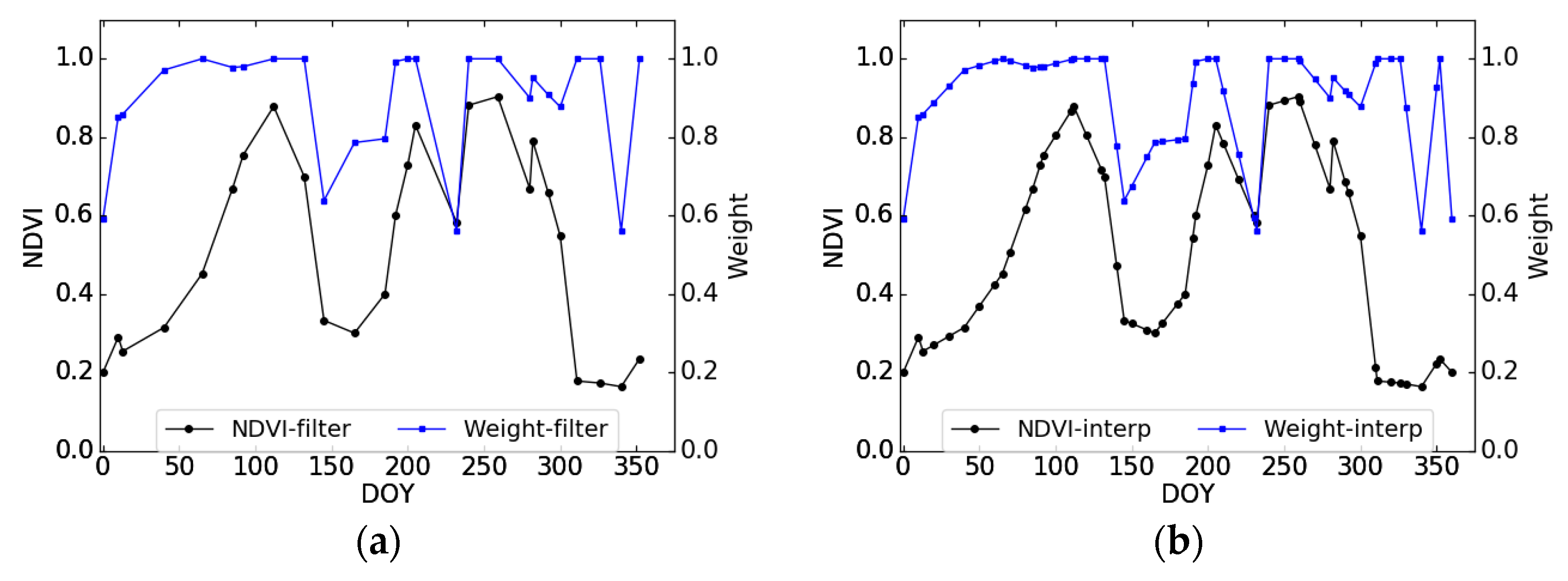
Just as the CLD value indicates the quality of the observed data, the ‘weight’ is introduced here as a quantitative indicator to describe the confidence level of each data point in the preprocessed TS ( N D V I p r e ). Specifically, weights for the originally observed data points from N D V I f i l t e r are calculated (Figure 5a) using the constructed relationship in the quadratic function form as
w k = ( 1 C L D k / 100 ) 2 ,
where C L D k is the CLD value of the k th data point of the N D V I f i l t e r . The calculated weights constitute a series of weight, where the weight of totally cloud-free data is 1.0, and contaminated data points are assigned with low weights.
Furthermore, to make a one-to-one match between the NDVI TS and the weight series, similarly, linear interpolation is applied to acquire a highly intensive weight series (Figure 5b). The weight of the interpolated data point is correlated to the confidence of two neighboring data points.
3. Identification of key temporal points for growth and senescence
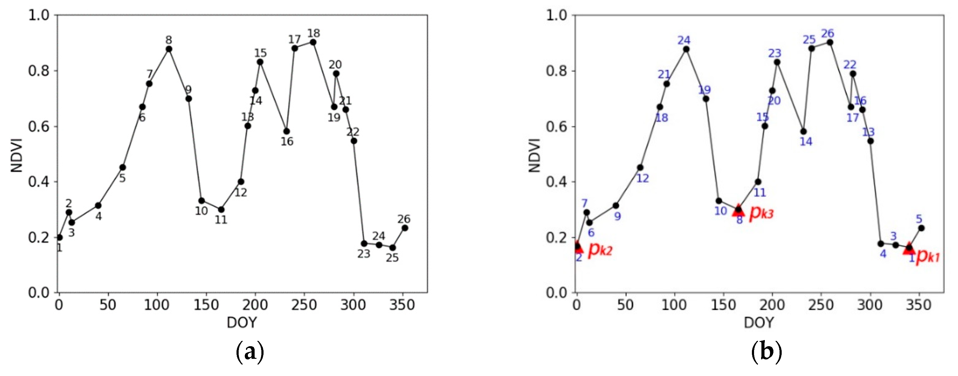
The key temporal point (pk) refers to the local minimum point. Key temporal points segment the global TS into subparts, each of which indicates a growth cycle. To search for pk, we traverse the N D V I f i l t e r points in the order from lowest to highest. First, the TS data points are sorted in ascending order (Figure 6). As shown, point 25 (Figure 6a) is the lowest and is marked as pk1 (Figure 6b). Then, the other points are traversed to search for pk2. If the point pair [pk1, pi] satisfies the following demands, pi is marked as pk2: the time span between pk1 and pi is longer than 90 days, which indicates a whole growth cycle, and the local amplitude is greater than 0.2. In that instance, point 1 (Figure 6a) meets the required conditions and is marked as pk2. After that, the identification of pk3 follows. Consequently, we can identify all key temporal points. As shown, the one-year NDVI TS of the double-season cropland contains three key temporal points, taking the whole TS into two adjacent subparts.
4. Weighted double-logistic function fitting
We use the weighted double-logistic function (WDL) function to fit the data points of each local segment. The difference of WDL and normal double-logistic (DL) method is that, in the proposed method, the importance of cloud-free data is enhanced, while the weights of contaminated data are lowered. The main problem to be solved is to find the optimized double-logistic function parameters ( p = [ a 1 , b 1 , c 1 , d 1 , a 2 , b 2 , c 2 , d 2 , e ] ) to model the growth process:
y = c 1 1 + e a 1 + b 1 t + d 1 + c 2 1 + e a 2 + b 2 t + d 2 e ,
The parameter derivation includes two steps: The initiation step and the iteration step, as shown in Figure 7.
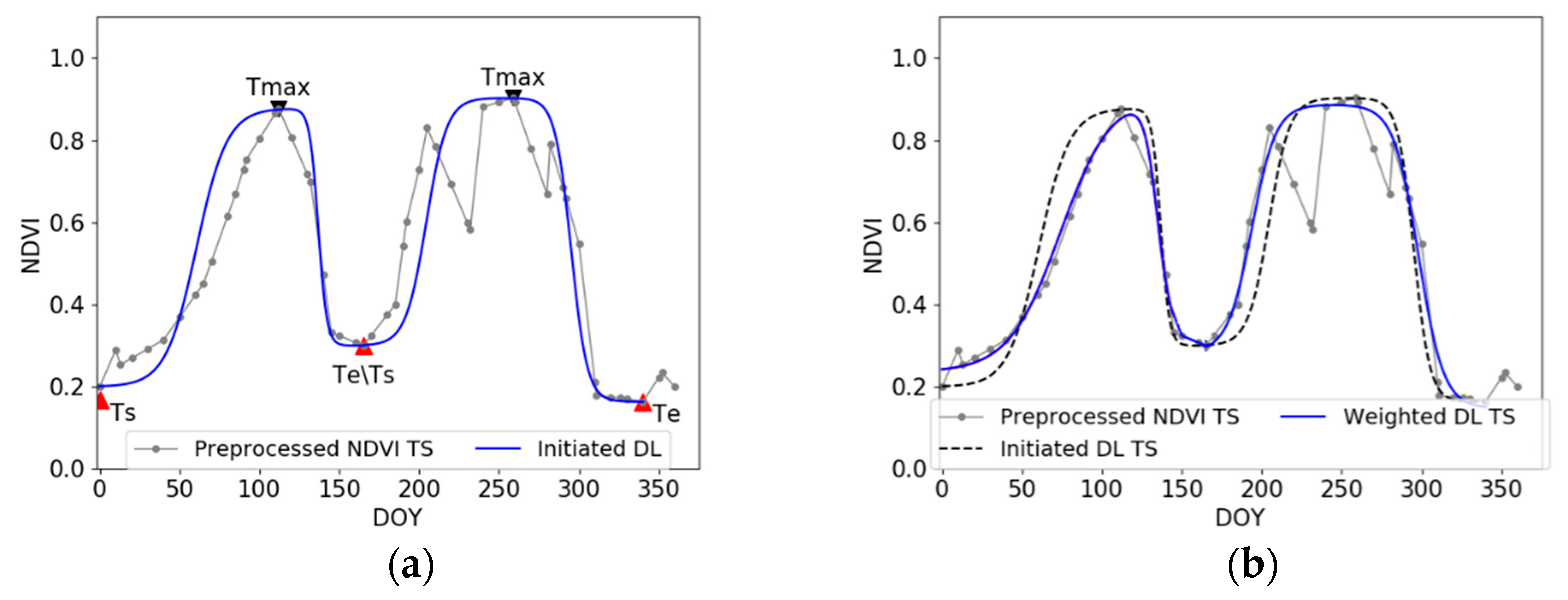
• Initiation step: The aim of the initiation step is to find a set of parameters which can approximately model the local TS with double-logistic function. The vegetation growth activity can be separated into two main parts (Figure 7a), namely, the growing part (from T s to T max ) and the declining part (from T max to T e ) (Equation (5)):
{ f 1 = c 1 1 + e a 1 + b 1 t + d 1 ,    T s t   T max f 2 = c 2 1 + e a 2 + b 2 t + d 2 ,    T max   < t T e ,
where d and c + d denote the minimum value (min(f)) and maximum value (max(f)), respectively; c indicates the local amplitude; and a and b determine the shape and slope of the logistic function graph, respectively. The subscripts 1 and 2 identify the parameters of the growing and declining parts, respectively. In the retrieval of these unknown parameters, the initial d and c are assigned as min(f) and max(f)-min(f), respectively. Thus, the principal problem is to derive parameters a and b . Considering the different weights of each of the data points, we transform the non-linear fitting problem into a linear one by a function transformation as a 1 + b 1 t = In ( c 1 f 1 d 1 1 ) . Furthermore, the weighted least squares (WLS) method is applied to solve the analytic expression of the logistic function for each part ( f 1 and f 2 ). It aims to minimize the weighted sum of squared residuals between the observed dependent variables and the predicted values:
arg min β i = 1 m w ii | y i j = 1 n X ij β j | 2 =   arg min β W 1 / 2 y X β 2   ,
where β = [ a b ] ; X = [ 1 X 11 1 X m 1 ] , where X m 1 is the actual independent variable data; y is [ y 1 y m ] , where elements are from the transformed dependent values In ( c N D V I i n t e r p d 1 ) ; m is the number of data points of N D V I i n t e r p ; n is the number of parameters to be solved (n = 2); W = [ w 1 0 0 0 0 0 0 w m ] , which is the diagonal weight matrix where the elements are from W i n t e r p . The gradient Equation (6) for the weighted squared sum leads to the solution of coefficient β .
After that, they are connected and expressed by a DL function (Figure 7a) in the form of Equation (4), where e = max ( c 1 + d 1 ,   c 2 + d 2 ) .
However, the generated results not only change the exact values of the original observations, but also alter the original seasonal variations of vegetation growth.
• Iteration step: Based on the initiated performance, the optimizing process is continued to promote the overall fitting effect. The aim is to maintain original observations and seasonal variations by minimizing the weighted sum of residual squares between the preprocessed data and the estimates (Equation (7)):
m i n   χ 2 = m i n   i w i [ y ( t i | p s ) y i ] 2 ,
where p s = [ a 1 , b 1 , c 1 , d 1 , a 2 , b 2 , c 2 , d 2 , e ] . The Gauss-Newton algorithm is applied to solve the nonlinear squares problem with nine unknown parameters. During the iteration step, c 1 , d 1 , c 2   and   d 2 are fixed, and p = [ a 1 , b 1 , a 2 , b 2 ,   e ] is noted as a changeable parameter set that needs to be optimized. For the convenience of expression, p is written as p = ( p 1 , p 2 p j p M ) T . The basic item of the parameter increment Δ p is
Δ p = ( J T WJ ) 1 J T W r ,
where J = [ f ( x 1 | p ) p 1 f ( x 1 | p ) p M f ( x N | p ) p 1 f ( x N | p ) p M ] , W = [ w i 0 0 w N ] .
J is a Jacobian matrix, which consists of the partial derivatives of the current model parameters; r is the residual data; W is the diagonal matrix, with entries from the current weight series. The initial W is determined by the weight series W pre . In each iteration step, the parameters are updated as:
p p + Δ p α ,
where the step length α is set as 0.05. Meanwhile, the weight matrix is also iteratively reassigned as
w i = { 1 ( y i y ^ i ) 2 ,    y ^ i y i > λ L 1 λ L 2 , y ^ i y i λ L   ,
where y i is the observed NDVI value, y ^ i is the predicted value and λ L is the median of the absolute residuals. A data point with small absolute residual is assigned with a higher weight. The weight of the outlier ( y ^ i y i > λ L ) can be effectively decreased through the thresholding strategy.
The iteration steps are terminated when the following conditions are satisfied: The mean squared errors (MSE = ( y ^ i y i ) 2 / N ) between the last two iterations (( k 1 )th and k th) are almost identical: | M S E k M S E k 1 | < 10 9 . The last iteration (the k th) reaches the optimized result (Figure 7b).

3. Results

We compared the proposed method with two representative TS filtering methods: The S-G and HANTS methods. Generally, for the S-G filter, a higher window size and a lower polynomial degree can well fetch the main temporal trend of the TS at the expense of smoothing the turning points. By contrast, a lower window size and a higher polynomial degree may overfit the TS and retain redundant noises. In our comparison experiments, we set the polynomial degree as three, and set the window size as three and five in two individual experiments, which are marked as SG-WS3 and SG-WS5, respectively. The HANTS algorithm smooths the TS by superimposing a series of sines and cosines and an additive item. More frequency components may bring more noise to the filtering effects. Three and five frequencies are selected from the Fourier spectrum in two comparison experiments, which are marked as HANTS-Freq3 and HANTS-Freq5, respectively. For the convenience of comparing these results clearly, SG-WS3 and HANTS-Freq5 are shown below. The qualitative and quantitative assessment results are presented as follows.

3.1. Qualitative Assessment

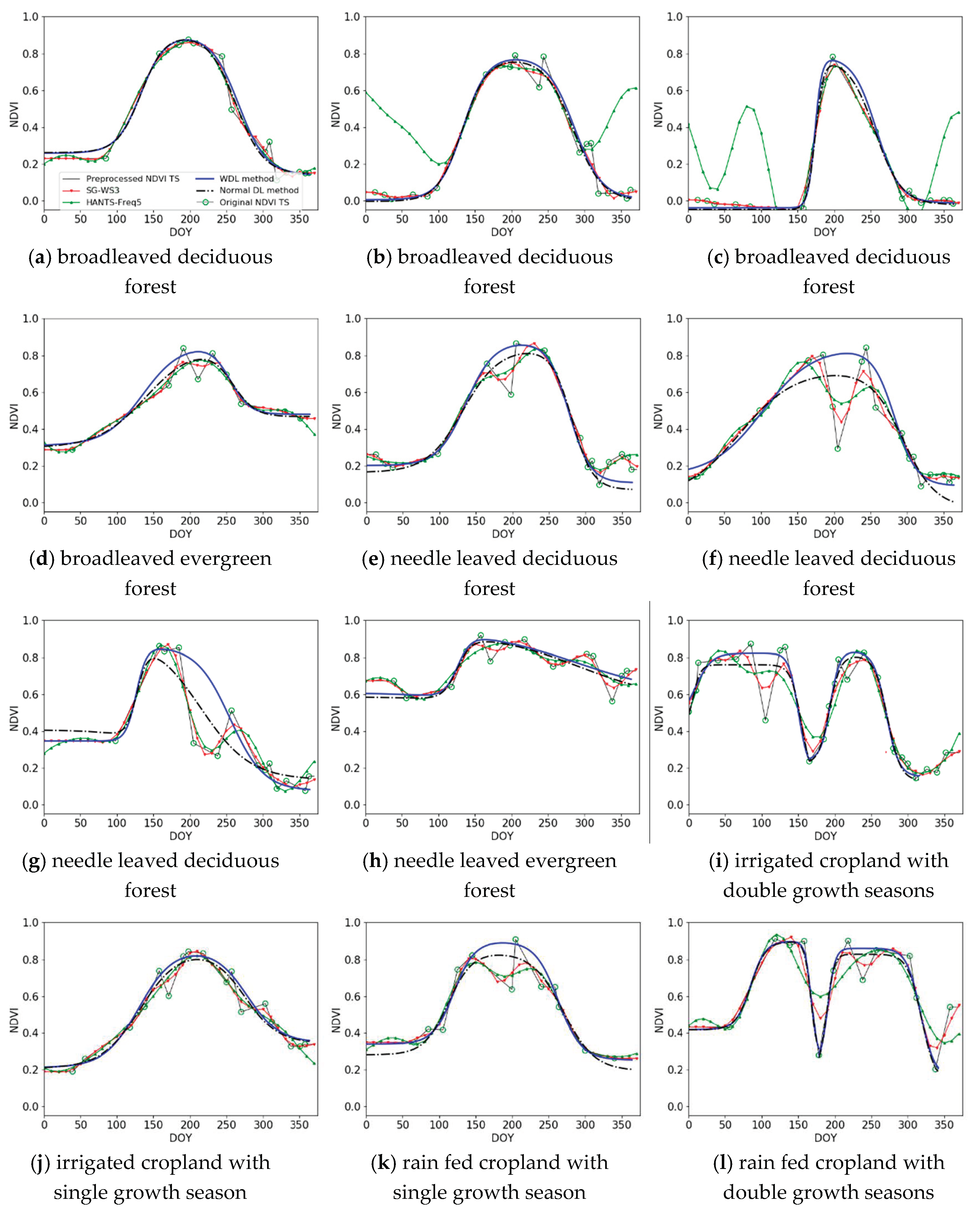
As shown in Figure 8, these three representative methods can generally capture TS temporal trends well, but differences exist in the details.
For a TS (e.g., Figure 8a,j,o) in a simple form with a single peak or little noise, the three methods perform well. When these methods are applied to complex TS (e.g., Figure 8f,g,i,m), which have double peaks or interference points, various filtering effects emerge. Compared to the proposed WDL method, the normal DL method cannot identify the cloud-contaminated data points, and the filtering result is greatly affected by the interference points, generally flattening high points (e.g., Figure 8f,g,k). As a result, significant vegetation growth information is lost, the original shape of the curve cannot be preserved well, and the growth durations are shorter than the original observations show (e.g., Figure 8g,n). For TS (e.g., Figure 8i,l) that represent double growth seasons, the HANTS method can capture the main temporal trend, but it flattens important peak points and wrongly raises successive low points, making the presented phenological characteristics unreliable (e.g., Figure 8i,l). Additionally, the component number coefficient has influence on the filtering effects. Coefficients should be adjusted for different situations, or the improper excessive components may produce nonexistent growth cycles (Figure 8b,c). HANTS has the advantage of capturing main temporal dynamics, but the proper coefficient is difficult to determine. As for S-G filtering results, the S-G method can smooth out abnormal slight fluctuations, and the produced TS is close to the original dynamic trend. Nevertheless, outliers bring much inaccuracy to S-G filtering effects (e.g., Figure 8f,g,k,m).
In our proposed WDL method, the segmentation procedure can effectively avoid a smoothing off of transitional low points (e.g., Figure 8i,l), and the weight reassignment strategy iteratively reduces the weights of the low points, and then successfully identifies outliers which are missed out in the preprocessing procedure (Figure 8f,n). On the contrary, when solving the uncertain points, this HANTS method is implemented by substituting outliers with newly predicted values. The drawback of the substitution is that if the new value deviates from the real seasonal variability, it may lead to a more deviating tendency.

3.2. Quantitative Assessment

The quantitative assessment method proposed by Hird et al. ([16]) was used to compare the de-noising performance of different TS filtering techniques. First, by means of computing averages of the filtered TS obtained from different methods (WDL, HANTS-Freq5 and SG-WS3), the synthesized ideal model was generated. Then we introduced various levels of noise to the ideal model. Specifically, low, medium and high levels of noise represent that 10%, 40% and 70% of the TS data points were respectively reduced by a random selection of 5%–50%, with an interval of 5%. The additions of noise simulated the TS under various contamination situations. Finally, these filtering methods were performed on the newly generated noised TS, and RSME was used to make a quantitative assessment of their de-noising abilities.
Table 2 shows the RMSE statistics for the three filtering methods after introducing different levels of noise into the original observed NDVI TS. These methods perform best when de-noising the TS with low level of noise. The noise reduction ability of WDL proves the best among the three methods because of the lowest RMSEs, on each situation with different levels of noise. Compared to T50SMB and T49REQ, WDL obtains the lowest RMSEs in the T51UVU, since that the dominant vegetation is the needle leaved deciduous forest, which has obvious phenological characteristics. The simple form of NDVI TS brings convenience to the noise reduction.

3.3. Reconstruction of High-Quality NDVI Time Series

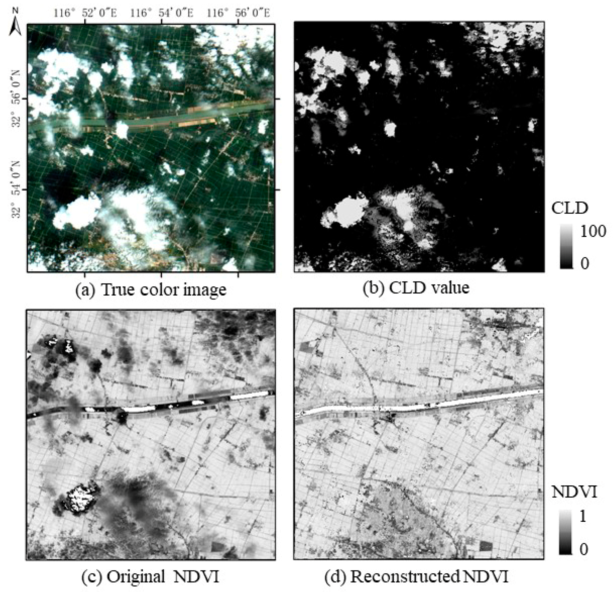
In this section, the proposed method is applied in a subset of the TS data set of tile T50SMB. According to a field survey in the study area, we collected the information about crop type, agricultural management like sowing date and growth stages of the crops. It is shown that this area is covered by paddy rice and the vegetation phenology is similar around. The remotely-sensed image acquired on August 28 is contaminated by clouds (Figure 9a). The atmospheric disturbance makes the NDVI values of the severely contaminated pixels extremely low (Figure 9b,c), and thus, the surface information is severely obscured. The WDL method reconstructs a high-quality NDVI TS, and the NDVI values of the cloud-contaminated pixels are successfully recovered (Figure 9d). The similar values between the cloud-free pixels and the cloud-contaminated pixels can further indicate the effectiveness and applicability of the proposed method.

4. Discussion

4.1. The Fidelities of High Data Points

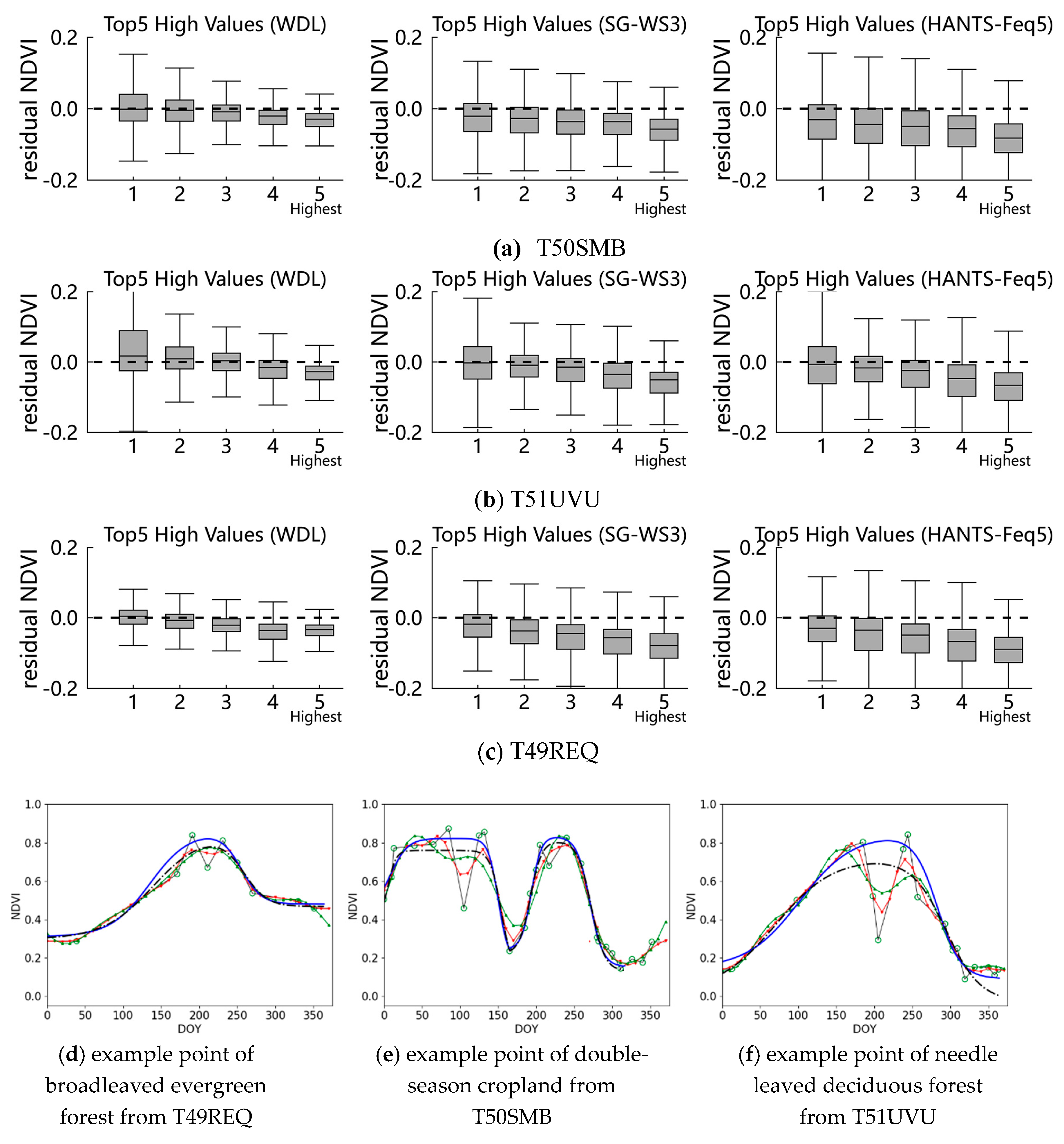
In this part, the fidelities of the methods are compared, which is implemented by statistics of residuals between the estimated and observed values. Obviously, high data points indicate the maturity stage of vegetation, while low data points represent the soil background or the cloud contamination. As shown by the qualitative assessment in the Results, the performance of the S-G and HANTS methods are greatly affected by contaminated data points, and in the filtered TS, high points cannot be well captured because of the neighboring contaminated data points. It caused the flattening of high data points, and may further cause error in the estimation of growth duration. Thus, for the sake of quantifying their abilities of maintaining high data points, we performed a quantitative method to describe the fidelities of high data points for these filtering techniques. They are evaluated in three study areas where the dominant vegetation types are different. Specifically, 548 broadleaved evergreen forest points in the T49REQ tile, 855 cropland points in the T50SMB tile and 752 needle leaved deciduous forest points in the T51UVU tile, are selected. It is obvious that even for the same land cover type, the vegetation may have various phenological characteristics and show different seasonal variability. The residuals between the estimated and observed values for the five highest (Top5 high) observation values are selected and analyzed. A positive residual indicates overestimation, while a negative residual indicates underestimation. The bars and whiskers in Figure 10 indicate the quantiles and value ranges, respectively. Figure 10 shows that compared to the other two methods, the WDL method yields median residuals that are generally closest to zero, and the bars are shorter for several of the highest values. The WDL method demonstrates its more stable performance in maintaining high values, which is also indicated by Table 3.
Table 3 shows that the HANTS filtering method performs worst, since the residuals are lower than the others, which means it can hardly trace the original NDVI observations. In respect to the S-G methodology, the effect of the S-G method should closely approach the original time series. However, it shows that the results of the S-G smoothing method always deviate from the original high values, although it appears to be slightly better than HANTS. These conclusions are consistent with the results in Figure 8.
In these study areas, there exist various time profile forms for the vegetation in the study areas, including a double-peak form for cropland with a two growth cycle, a one-peak form for needle leaved deciduous forest, and successive high NDVI values with slight dynamic changes for broadleaved evergreen forest. The WDL methods shows absolutely higher performance in the fidelity of high data points than the other methods because of the low RMSEs.

4.2. Discussion of the Number of Iterations

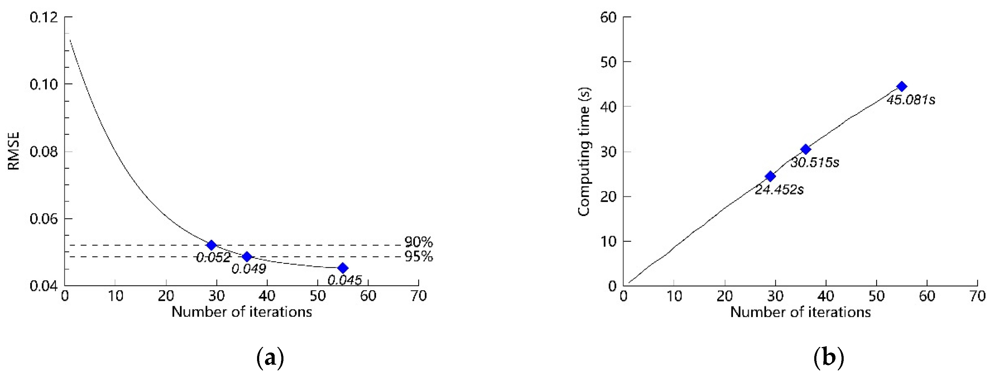
As analyzed in the methods section, more iterations for searching the optimal parameter set can make the model approach the optimized result more closely, but take more computing time. In this section, we quantitatively evaluate the effect of iterations on the fitting accuracy and the computing time. The RMSEs of the estimated and observed values are applied as indicators of the model performance. Specifically, the RMSE is the mean value for the test points, and the computing time is the total value. Figure 11a. indicates that the RMSE declines rapidly in the first few iterations and then changes slowly. The RMSE decreases from an initial status of 0.113, and terminates with a result of 0.045. The iterations produce a decrease of 0.068 for the RMSE and take 45.081 s (Figure 11b). Figure 11b shows that the computing time is nearly proportional to the number of iterations. However, a small sacrifice to the fitting accuracy can save much time.
For instance, if the iterative processes are terminated when the decrease reaches 95%, they take only 30.515 s. Similarly, much more time can be saved when the threshold is set to 90%. The above quantitative analysis result provides information on how to set an appropriate number of iterations in later use.

5. Conclusions

The NDVI TS has been widely used in land-surface dynamics monitoring. However, atmospheric disturbances and other influencing factors cause noise and obscure further applications of the NDVI TS. Taking the Sentinel-2 NDVI TS data set as an example, this paper proposes applying the weighted double-logistic method to reconstruct a high-quality NDVI TS data set with medium spatial resolution.
First, the preprocessing procedure is performed as a fundamental step, which produces highly intensive NDVI time profiles in which obvious outliers have been preliminarily filtered out. Then, the rule-based strategy is adopted to identify key temporal points that segment global TS into local parts. Then, the data points of each local part are fitted using the WDL function. In the iteration steps for searching the optimized parameter set, cloud-contaminated data are assigned with low weights, and cloud-free data play larger roles.
The proposed method has at least three advantages: First, the introduction of weighted data into the filtering process effectively recognizes abnormal low outliers and enhances the importance of reliable data points. By contrast, without weight, the normal DL filtering method is likely to raise low values and flatten high values. Second, in comparison with the S-G and HANTS filtering methods, the newly developed method can identify significant turning points and acquire a local optimization of each growth season. By comparison, the S-G method is likely to flatten important turning points due to its methodology, and the HANTS result tends to deviate far from the original TS shape and amplitude, especially for curves with complex forms. Third, according to quantitative assessment, the proposed method can well maintain high values.
The limitations of the proposed method mainly exist in the following aspects: On the one hand, the cloud indicator CLD is applied to weight the data points in the research. However, sometimes it cannot accurately represent the effects that are caused by disturbance factors. On the other hand, when filtering the NDVI TS of vegetation, the dynamic changes of which are slight, the method can hardly capture the variations.
In summary, the proposed methods make contributions on generating a high-quality NDVI time series based on medium-resolution remote sensing images. The reconstructed NDVI time series is significant for monitoring the seasonal variability of vegetation, and the dynamic change of land surface.

Author Contributions

Y.Y. proposed the research methodology, designed and performed the experiments, and wrote the manuscript. Q.H. helped in formal analysis and validation. W.W. had great contributions on the manuscript review and editing. J.L. outlined the research topic and acquired the funding. Y.S. had contributions to data preparation and analysis.

Funding

This study was funded by the National Key Research and Development Program of China (Grant No. 2017YFB0503600), and the National Natural Science Foundation of China (Grant No. 41631179).

Acknowledgments

We thank ESA Copernicus Open Access Hub for providing the Sentinel-2 data used in this study. We also thank peer reviewers and the academic editor for providing useful comments and good suggestions.

Conflicts of Interest

The authors declare no conflict of interest.

References

  1. Atzberger, C.; Eilers, P.C. A time series for monitoring vegetation activity and phenology at 10-daily time steps covering large parts of South America. Int. J. Digit. Earth 2011, 4, 365–386. [Google Scholar] [CrossRef]
  2. Beck, P.S.A.; Atzberger, C.; Høgda, K.A.; Johansen, B.; Skidmore, A.K. Improved monitoring of vegetation dynamics at very high latitudes: A new method using MODIS NDVI. Remote Sens. Environ. 2006, 99, 321–334. [Google Scholar] [CrossRef]
  3. Tucker, C.J.; Eldin, J.H., Jr.; Iii, M.M.; Fan, C.J. Monitoring corn and soybean crop development with hand-held radiometer spectral data. Remote Sens. Environ. 1979, 8, 237–248. [Google Scholar] [CrossRef]
  4. Guyon, D.; Guillot, M.; Vitasse, Y.; Cardot, H.; Hagolle, O.; Delzon, S.; Wigneron, J.P. Monitoring elevation variations in leaf phenology of deciduous broadleaf forests from SPOT/VEGETATION time-series. Remote Sens. Environ. 2011, 115, 615–627. [Google Scholar] [CrossRef]
  5. Atkinson, P.M.; Jeganathan, C.; Dash, J.; Atzberger, C. Inter-comparison of four models for smoothing satellite sensor time-series data to estimate vegetation phenology. Remote Sens. Environ. 2012, 123, 400–417. [Google Scholar] [CrossRef]
  6. Leeuwen, W.J.D.V.; Hartfield, K.; Miranda, M.; Meza, F.J. Trends and ENSO/AAO Driven Variability in NDVI Derived Productivity and Phenology alongside the Andes Mountains. Remote Sens. 2013, 5, 1177–1203. [Google Scholar] [CrossRef] [Green Version]
  7. Zeng, H.; Jia, G.; Forbes, B.C. Shifts in Arctic phenology in response to climate and anthropogenic factors as detected from multiple satellite time series. Environ. Res. Lett. 2013, 8, 035036. [Google Scholar] [CrossRef]
  8. Xiao, X.; Boles, S.; Frolking, S.; Li, C.; Babu, J.Y.; Salas, W.; Iii, B.M. Mapping paddy rice agriculture in South and Southeast Asia using multi-temporal MODIS images. Remote Sens. Environ. 2006, 100, 95–113. [Google Scholar] [CrossRef]
  9. Chen, C.F.; Huang, S.W.; Son, N.T.; Chang, L.Y. Mapping double-cropped irrigated rice fields in Taiwan using time-series Satellite Pour I’Observation de la Terre data. J. Appl. Remote Sens. 2011, 5, 3528. [Google Scholar] [CrossRef]
  10. Patakamuri, S.K. Time-Series analysis of MODIS NDVI data along with ancillary data for Land use/Land cover mapping of Uttarakhand. ISPRS-Int. Arch. Photogramm. Remote Sens. Spat. Inf. Sci. 2014, XL-8, 1491–1500. [Google Scholar] [CrossRef] [Green Version]
  11. Defries, R.S.; Townshend, J.R.G. NDVI-derived land cover classifications at a global scale. Int. J. Remote Sens. 1994, 15, 3567–3586. [Google Scholar] [CrossRef]
  12. Arvor, D.; Jonathan, M.; Dubreuil, V.; Durieux, L. Classification of MODIS EVI time series for crop mapping in the state of Mato Grosso, Brazil. Int. J. Remote Sens. 2011, 32, 7847–7871. [Google Scholar] [CrossRef]
  13. Rodrigues, A.; Marcal, A.R.S.; Furlan, D.; Ballester, M.V.; Cunha, M. Land cover map production for Brazilian Amazon using NDVI SPOT VEGETATION time series. Can. J. Remote Sens. 2013, 39, 277–289. [Google Scholar] [CrossRef]
  14. Sellers, P.J.; Tucker, C.J.; Collatz, G.J.; Los, S.O.; Justice, C.O.; Dazlich, D.A.; Randall, D.A. A global 1° by 1° NDVI data set for climate studies. Part 2: The generation of global fields of terrestrial biophysical parameters from the NDVI. Int. J. Remote Sens. 1994, 15, 3519–3545. [Google Scholar] [CrossRef]
  15. Möller, M.; Gerstmann, H.; Dahms, T. Phenological NDVI time series for the dynamic derivation of soil coverage information. In Proceedings of the IEEE International Geoscience and Remote Sensing Symposium, Fort Worth, TX, USA, 23–28 July 2017; pp. 4278–4281. [Google Scholar]
  16. Hird, J.N.; Mcdermid, G.J. Noise reduction of NDVI time series: An empirical comparison of selected techniques. Remote Sens. Environ. 2009, 113, 248–258. [Google Scholar] [CrossRef]
  17. Chen, J.; Jönsson, P.; Tamura, M. A simple method for reconstructing a high-quality NDVI time-series data set based on the Savitzky–Golay filter. Remote Sens. Environ. 2004, 91, 332–344. [Google Scholar] [CrossRef]
  18. Julien, Y.; Sobrino, J.A. Global land surface phenology trends from GIMMS database. Int. J. Remote Sens. 2009, 30, 3495–3513. [Google Scholar] [CrossRef] [Green Version]
  19. Zhou, J.; Jia, L.; Menenti, M.; Gorte, B. On the performance of remote sensing time series reconstruction methods—A spatial comparison. Remote Sens. Environ. 2016, 187, 367–384. [Google Scholar] [CrossRef]
  20. Holben, B. Characteristics of maximum-value composite images from temporal AVHRR data. Int. J. Remote Sens. 1986, 7, 1417–1434. [Google Scholar] [CrossRef]
  21. Yang, G.; Shen, H.; Zhang, L.; He, Z.; Li, X. A Moving Weighted Harmonic Analysis Method for Reconstructing High-Quality SPOT VEGETATION NDVI Time-Series Data. IEEE Trans. Geosci. Remote Sens. 2015, 53, 6008–6021. [Google Scholar] [CrossRef]
  22. Viovy, N.; Arino, O.; Belward, A.S. The Best Index Slope Extraction ( BISE): A method for reducing noise in NDVI time-series. Int. J. Remote Sens. 1992, 13, 1585–1590. [Google Scholar] [CrossRef]
  23. Lovell, J.L.; Graetz, R.D. Filtering Pathfinder AVHRR Land NDVI data for Australia. Int. J. Remote Sens. 2001, 22, 2649–2654. [Google Scholar] [CrossRef]
  24. Ma, M.; Veroustraete, F. Reconstructing pathfinder AVHRR land NDVI time-series data for the Northwest of China. Adv. Space Res. 2006, 37, 835–840. [Google Scholar] [CrossRef]
  25. Savitzky, A.; Golay, M.J.E. Smoothing and Differentiation of Data by Simplified Least Squares Procedures. Anal. Chem. 1964, 36, 1627–1639. [Google Scholar] [CrossRef]
  26. Jonsson, P.; Eklundh, L. Seasonality extraction by function fitting to time-series of satellite sensor data. IEEE Trans. Geosci. Remote Sens. 2002, 40, 1824–1832. [Google Scholar] [CrossRef]
  27. Fisher, J.I.; Mustard, J.F.; Vadeboncoeur, M.A. Green leaf phenology at Landsat resolution: Scaling from the field to the satellite. Remote Sens. Environ. 2006, 100, 265–279. [Google Scholar] [CrossRef]
  28. Zhang, X.; Friedl, M.A.; Schaaf, C.B.; Strahler, A.H.; Hodges, J.C.F.; Gao, F.; Reed, B.C.; Huete, A. Monitoring vegetation phenology using MODIS. Remote Sens. Environ. 2003, 84, 471–475. [Google Scholar] [CrossRef]
  29. Hermance, J.F.; Jacob, R.W.; Bradley, B.A.; Mustard, J.F. Extracting Phenological Signals From Multiyear AVHRR NDVI Time Series: Framework for Applying High-Order Annual Splines With Roughness Damping. IEEE Trans. Geosci. Remote Sens. 2007, 45, 3264–3276. [Google Scholar] [CrossRef]
  30. Geerken, R.; Zaitchik, B.; Evans, J.P. Classifying rangeland vegetation type and coverage from NDVI time series using Fourier Filtered Cycle Similarity. Int. J. Remote Sens. 2005, 26, 5535–5554. [Google Scholar] [CrossRef]
  31. Verhoef, W. Application of harmonic analysis of NDVI time series (HANTS). Fourier Anal. Temporal NDVI South. Afr. Am. Cont. 1966, 108, 19–24. [Google Scholar]
  32. Evans, J.P.; Geerken, R. Classifying rangeland vegetation type and coverage using a Fourier component based similarity measure. Remote Sens. Environ. 2006, 105, 1–8. [Google Scholar] [CrossRef]
  33. Crist, E.P.; Malila, W.A. A temporal-spectral analysis technique for vegetation applications of Landsat. In Proceedings of the International Symposium on Remote Sensing of Environment, San Jose, CA, USA, 23–30 April 1980. [Google Scholar]
  34. Fischer, A.; Kergoat, L.; Dedieu, G. Coupling satellite data with vegetation functional models: Review of different approaches and perspectives suggested by the assimilation strategy. Remote Sens. Rev. 1997, 15, 283–303. [Google Scholar] [CrossRef]
  35. Available online: https://earth.esa.int/web/sentinel/technical-guides/sentinel-2-msi/level-2a/algorithm (accessed on 6 October 2019).
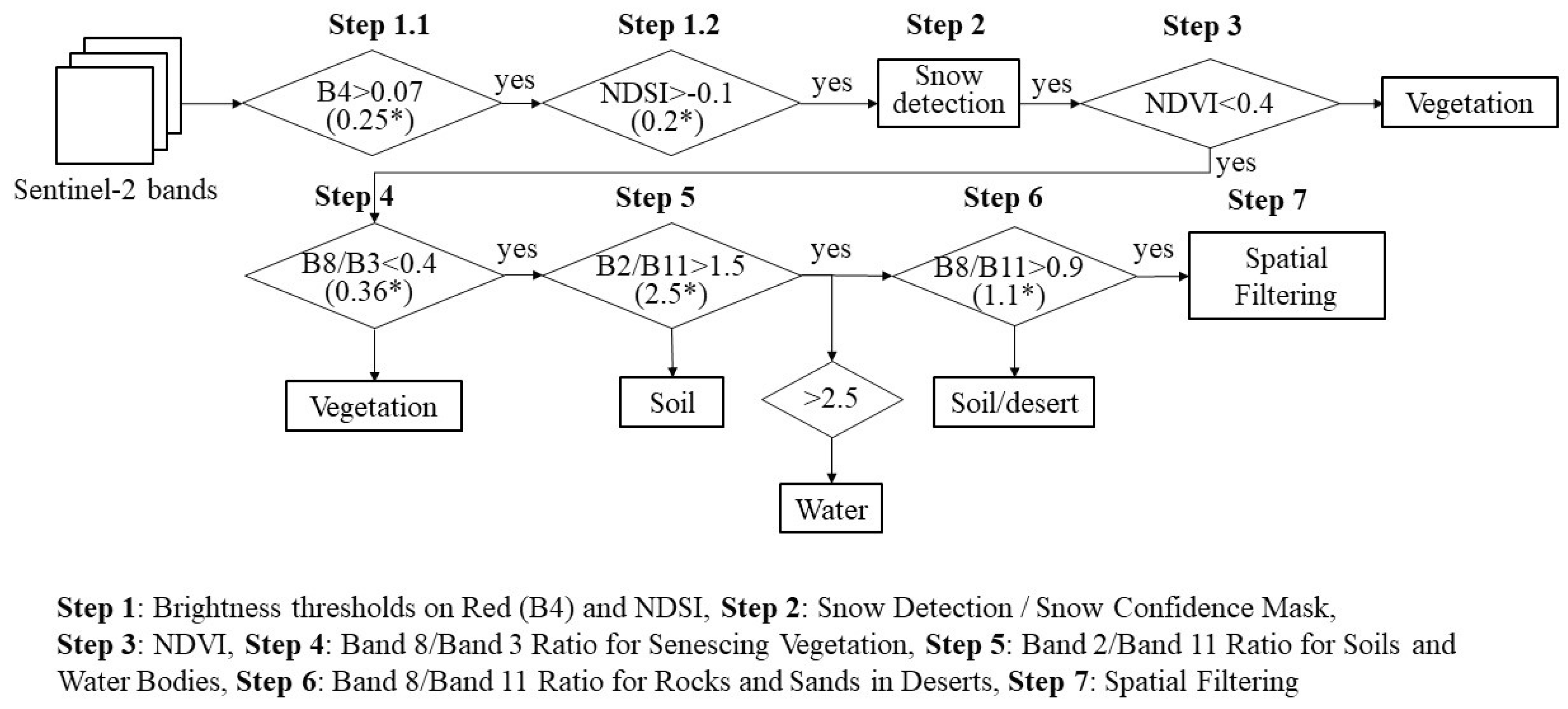
Figure 1. Cloud detection and cloud probability calculation.
Remotesensing 11 02342 g001
Figure 2. Sentinel-2 satellite data, zoom-in images from Google Earth, and land cover types of the three study areas.
Remotesensing 11 02342 g002
Figure 3. The flowchart of the proposed method.
Remotesensing 11 02342 g003
Figure 4. Example of the preprocessing procedure in the present method. (a) Original normalized difference vegetation index time series (NDVI TS) and cloud mask quality indicator file time series (CLD TS). (b) TS after filtering out poor-quality cloud-contaminated points. (c) TS after removing the identified outlier (i.e., N D V I f i l t e r ). (d) The preprocessed NDVI TS (i.e., N D V I p r e ).
Remotesensing 11 02342 g004
Figure 5. (a) NDVI TS N D V I f i l t e r and the calculated weight series W f i l t e r . (b) The interpolated NDVI TS and the interpolated weight series.
Remotesensing 11 02342 g005
Figure 6. (a) The N D V I f i l t e r labeled with the observation sequence. (b) The N D V I f i l t e r labeled with the sorted orders and the identified key temporal points.
Remotesensing 11 02342 g006
Figure 7. (a) Preprocessed NDVI TS of a one-year double-season cropland and the initiated DL function. The identified key temporal points (red triangles) and local maximum points (black inverted triangles) have been marked. (b) The local fitting results after the optimization process.
Remotesensing 11 02342 g007
Figure 8. Filtering results of the Savitzky-Golay (S-G), harmonic analysis of time series (HANTS), normal DL and proposed methods. The green circles show the original, non-cloudy observations, and the severely atmospherically-contaminated data points have been discarded. The results include various land cover types in the study areas: Including broadleaved deciduous forest, broadleaved evergreen forest, needle leaved deciduous forest, needle leaved evergreen forest, irrigated cropland, and rain fed cropland with one or double seasons, mosaic tree and shrub/herbaceous cover, mosaic cropland/natural vegetation, and grassland.
Remotesensing 11 02342 g008aRemotesensing 11 02342 g008b
Figure 9. Comparison between the original NDVI and the reconstructed NDVI values.
Remotesensing 11 02342 g009
Figure 10. Method comparison results of the three techniques in three study areas. (ac) show the NDVI residuals of Top5 high data points. The numbers along the x-axis represent the order from low to high values. (df) show the example points.
Remotesensing 11 02342 g010
Figure 11. (a) Relationship between the Root Mean Squared Error (RMSE) and the number of iterations. (b) Relationship between the computing time and the number of iterations.
Remotesensing 11 02342 g011
Table 1. Sampling point number for each class in each tile.
Land Cover TypeT50SMBT51UVUT49REQ
Rain fed cropland2231294
Irrigated cropland1676 415
Mosaic cropland/natural vegetation 192
Broadleaved evergreen forest 651
Broadleaved deciduous forest 228214
Needle leaved evergreen forest 394
Needle leaved deciduous forest 1701
Mosaic tree and shrub/herbaceous cover 18145
Grassland 83
Table 2. RMSE statistics for these de-noising methods.
Study AreaMethodLevels of Noise
LowMediumHigh
T50SMBWDL0.0460.0690.089
S-G0.0510.0880.115
HANTS0.0580.0880.114
T51UVUWDL0.0390.0610.083
S-G0.0430.0810.112
HANTS0.0550.0840.119
T49REQWDL0.0490.0740.098
S-G0.0530.0950.129
HANTS0.0530.0930.126
Table 3. RMSE statistics of Top5 high points for the three methods.
Study AreaMethodRMSE for Top5 High Points
12345 a
T50SMBWDL0.0530.0440.0330.0370.040
S-G0.0590.0600.0590.0590.073
HANTS0.0770.0840.0860.0880.101
T51UVUWDL0.0930.0460.0340.0410.041
S-G0.0730.0490.0500.0640.073
HANTS0.0810.0590.0670.0820.089
T49REQWDL0.0280.0300.0330.0470.042
S-G0.0520.0610.0740.0820.094
HANTS0.0620.0780.0870.0990.107
a RMSE for the highest data points.