Selection of the Key Earth Observation Sensors and Platforms Focusing on Applications for Polar Regions in the Scope of Copernicus System 2020–2030

 , , ,
, , ,
Abstract
1. Introduction
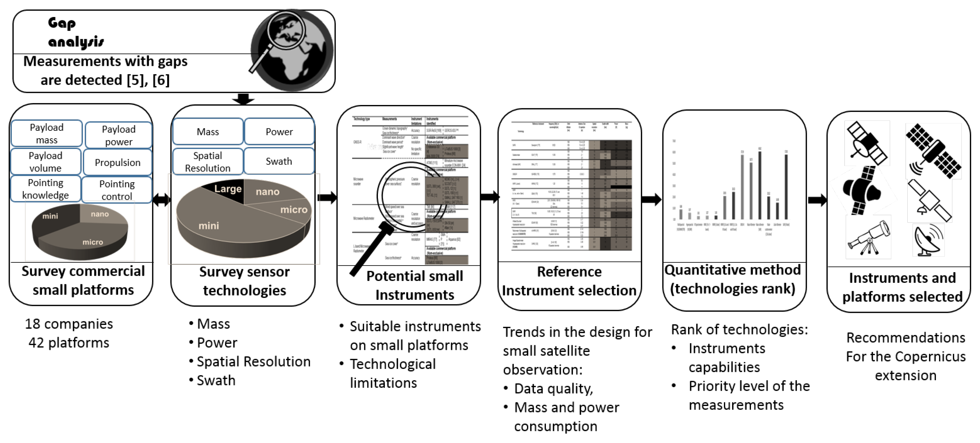
2. Survey of Commercial Small Platforms
3. Survey of Earth Observation Sensors and Measurements Requirements to Cover the Future Gaps on Copernicus
3.1. Passive Microwave
3.1.1. Microwave Imagers (MWIm)
- A Tropical Rainfall Measuring Mission Microwave Imager (TMI) like instrument is capable of measuring wind speed (at 10.65, 19.35 and 37 GHz), sea ice cover (at 19.35, 37, and 85.5 GHz), and sea surface temperature (at 10.65 GHz). Modified versions of TMI for micro- or mini-platforms achieving a 10 km spatial resolution using an aperture size (inflatable antenna) of 3.4 m @ 10.65 GHz from 600 km height will suit LEO polar Sun-Synchronous Orbit (SSO, ∼14 orbits/day) reducing the revisit time to 3 h in the Polar Regions. The required number of satellites was optimized in [31].
- The available L-Band microwave sensors, such as Microwave Imaging Radiometer using Aperture Synthesis (MIRAS) and Soil Moisture Active-Passive (SMAP) are suitable for mini-platforms. L-band microwave radiometers are capable of measuring the variables with the detected gaps, such as sea ice thickness and soil moisture. Sea ice thickness presents gaps in the revisit and latency times. The revisit time required is 24 h, and a latency time of 1 h. Surface soil moisture monitoring presents gaps in the accuracy 0.01 m/m and the latency time 1 h.
3.1.2. Microwave Sounders (MWS)
3.1.3. Signals of Opportunity (SoOp): GNSS-R, and Receiver of SoOp
3.1.4. Receiver: Automatic Identification System (AIS)
3.2. Passive Optical
3.2.1. Radiometer: Multispectral and Hyperspectral
3.2.2. Sounder: Multispectral and Hyperspectral
3.3. Active Microwave
3.3.1. Real Aperture Radar Altimeter
3.3.2. Real Aperture Radar Scatterometers
3.3.3. Synthetic Aperture Radar (SAR) Altimeter
3.3.4. Synthetic Aperture Radar (SAR) Imager
3.4. Active Optical
Lidar
- Atmospheric dynamics or horizontal winds, (e.g., ESA Atmospheric Dynamic Mission ADM-Aeolus [79] was launched on 22 August 2018). Lidar instruments present the following main characteristics:
- Operating wavelengths in the UV, VIS, NIR, and SWIR; possible dual-wavelength, polarimetry, and two receivers (for Mie and Rayleigh scattering).
- Spatial resolution in the range of 100 m to a few tens of centimeters for LIDAR altimeters.
- Non-scanning, either nadir-viewing or oblique.
4. Potential Instrument, Suitable Platforms, and Technological Limitations
- GNSS-R (1.4 kg, 12 W) instruments are suitable for nanosatellites (3U or 6U). Table 6 presents sample available commercial platforms for the SGR-ReSi [57], such as the Endeavour-3U [18] and the MAI-3000 [17]. Endeavour by Tyvak Nanosatellite Technology Inc. (San Luis Obispo, CA. United States of America), is a 3U platform with 15 W of average payload power, 3 deg of pointing control. MAI-3000 by Maryland Aerospace, is a 3U platform with 12 W of payload power and 3 kg of available payload mass. The main limitation of GNSS-R altimetry data is the poorer (decimetric) resolution and accuracy (∼20 cm for SSH, and 2 m/s for wind speed) are offset by the much larger number of simultaneous observations from different specular reflection points [80].
- Another good example are microwave sounders on small-platforms such as EON-MW [33], for measuring the atmospheric pressure over the sea surface. However, the antenna system must be redesigned to achieve the spatial resolution required. For a 10 km spatial resolution, at 50 GHz, the require antenna aperture is 36 cm, from an altitude of 600 km. Table 6 summarizes a list of the available commercial micro-platforms suitable for this instrument.
- Microwave imagers at X-, K-, Ka-, and W- bands are particularly well suited for implementation on small platforms (Table 6). TMI is a light instrument suitable for mini-satellites, with X-, K-, Ka-, and W- bands capable of measuring and covering the gaps for wind speed, sea ice cover, sea ice type, and sea surface temperature variables. For sea surface temperature, microwave radiometers improve the coverage in polar regions because of their all weather capabilities. In order to obtain a spatial resolution of 10 km at 18.7 GHz from 600 km height, a 2.2 m antenna is required. On the other hand, an SSM/I type of instrument with a modified antenna, could be implemented in a micro-platform in order to cover wind speed over the sea surface, sea ice cover, and sea ice measurements, with the required performance. L-band radiometers contribute to sea ice thickness monitoring, agriculture (soil moisture) and forestry measurements. Those instruments are suitable for mini-platforms (Table 6). The main limitation is their coarse resolution. Inflatable antennas must be used to reduce the footprint size, or aperture synthesis techniques could be implemented [81]. ELiTeBUS 1000 [10] by Thales Alenia Space (Cannes, France) is an available commercial small-platform suitable for this instrument. ELiTeBUS 1000 is a platform for Medium Earth Orbit (MEO) and Low Earth Orbit (LEO) orbit with 1000 to 1500 W of available payload power.
- Scatterometers contribute to the Marine for Weather Forecast and Sea Ice Monitoring use cases. The instrument taken as a reference is the SCAT on board the CFOSAT mission [25,82], the power consumption of this sensor is less than 200 W, and the mass less than 200 kg. According to the power consumption and mass requirements, this payload can be carried on board mini-platforms (Table 7). Scatterometers are valuable sensors for wind measurements. However, the main limitations are the coarse accuracy and spatial resolution of the data. However, their wide swath and the possibility of scatterometer constellations open the door to improve the accuracy and spatial resolution, combining the data from multiple passes of different satellites.
- For radar altimeters, the accuracy of the measurements depends on the Pulse Repetition Frequency (PRF), which is directly driven by the power available on-board to the payload. Since the power available on-board decreases with solar panel size, the accuracy of the measurements on a small satellite is also expected to be degraded as compared to that of large satellites. For example, if the power consumption is reduced by a factor of 4, the PRF is reduced roughly by the same factor, and the Root-Mean-Square (RMS) error increases by a factor of 2. For the Jason-2 altimeter (power consumption ∼70 W), a reduction of its power consumption to 1 W, would increase the sensor error level from 2 cm to ∼16.7 cm, which is actually comparable to GNSS-R [55,82]. It is easy to understand that the types of products that can be generated with this accuracy are different from the ones generated with an SRAL radar altimeter, but one must also consider that the number of radar altimeters with a transmitted power of 1 W that can be manufactured and launched at the same cost as for a high accuracy radar altimeter is much larger. These few examples illustrate the fact that the quality and frequency of the measurements have to be considered in the overall comparison process. In some cases, the concept of operations may partially be compensated by the degradation of the quality of the individual measurements (e.g., part-time measurement instead of systematic measurement if the power available on board is the main parameter driving the performance of the measurement).
- SAR sensors are one of the most effective instruments for ocean, land, and ice observation. A good example of miniaturization of this technology is the Severjamin-M instrument (Meteor-M N missions) [83], an X-band SAR with power consumption of 1 kW and a mass of 150 kg, including the mass of the antenna of 40 kg. The main technological limitation is the narrow swath, but this could be compensated with a constellation of SAR satellites.
- Optical payloads are characterized in terms of image quality such as the Ground Sampling Distance (GSD), the Modulation Transfer Function (MTF), and the Signal-to-Noise Ratio (SNR). To be able to interpret an image (e.g., in the maritime surveillance, the capability to estimate the type of a boat), the GSD is not sufficient, since a degraded MTF (i.e., blurred image) or a degraded SNR (noisier image) would prevent it. Ensuring a good MTF and SNR for a given GSD requires a minimum aperture for the optical instrument, and reducing it below this minimum value will limit the type of applications. Image quality is also limited by the platform’s attitude control system, i.e, any jitter in the pointing will blur the image. This has also to be taken into account as smaller platforms exhibit poorer performances.
5. Reference Instrument Selection
- SGR-ReSI instrument presents a good performance for sea ice cover [99] because it satisfies the minimum requirement for spatial resolution and accuracy. For ocean surface currents, and significant wave height measurements satisfy the minimum requirement of spatial resolution at 25 km [100]. For other measurements, such as sea ice thickness [46], soil moisture [101], and wind speed [80] present worse performance than the minimum spatial resolution and accuracy requirements.
- EON-MW is a satellite project under development and presents an approximate performance that the Advanced Technology Microwave Sounder (ATMS) [33], in this way, it will be expected that the instrument satisfies the minimum requirements for accuracy of 5% and spatial resolution at 23 km for atmospheric pressure over sea surface measurements (channel from 50 to 60 GHz).
- MIRAS instrument presents a coarse spatial resolution ∼35 × 50 km for horizontal- and vertical- polarization. This instrument has an accuracy of 0.04 m/m for soil moisture measurements [102] that is worse than 0.01 m/m required. For sea ice thickness, the accuracy is worse than the 1 cm required [103], but it can have an accuracy of 5% for sea ice cover.
- SSM/I using an antenna (inflatable) of 2.2 m from 600 km orbit altitude can obtain a spatial resolution of 10 km and satisfy the minimal spatial resolution requirement for wind speed, and sea ice cover measurements. The accuracy for wind speed measurement can be until 1.5 m/s [104], and for sea ice data from 10% to 20% [105].
- AVHRR/3 presents a spatial resolution ∼1 km, and computes an accuracy better than 0.1 K [106].
- EON-IR is expected to be better than 0.25 K and present, with spatial resolution at 13.5 km.
- SCAT—the accuracy for wind speed monitoring is 2 m/s, and for sea ice monitoring is 5%.
- Severjamin has a spatial resolution from 400 m to 1 km depending on the operation mode can satisfy many minimal requirements for some measurements.
- GLAS acquires the geophysical variables with a vertical spatial resolution of 10 cm, which does not satisfy the user requirement for sea ice thickness measurements.
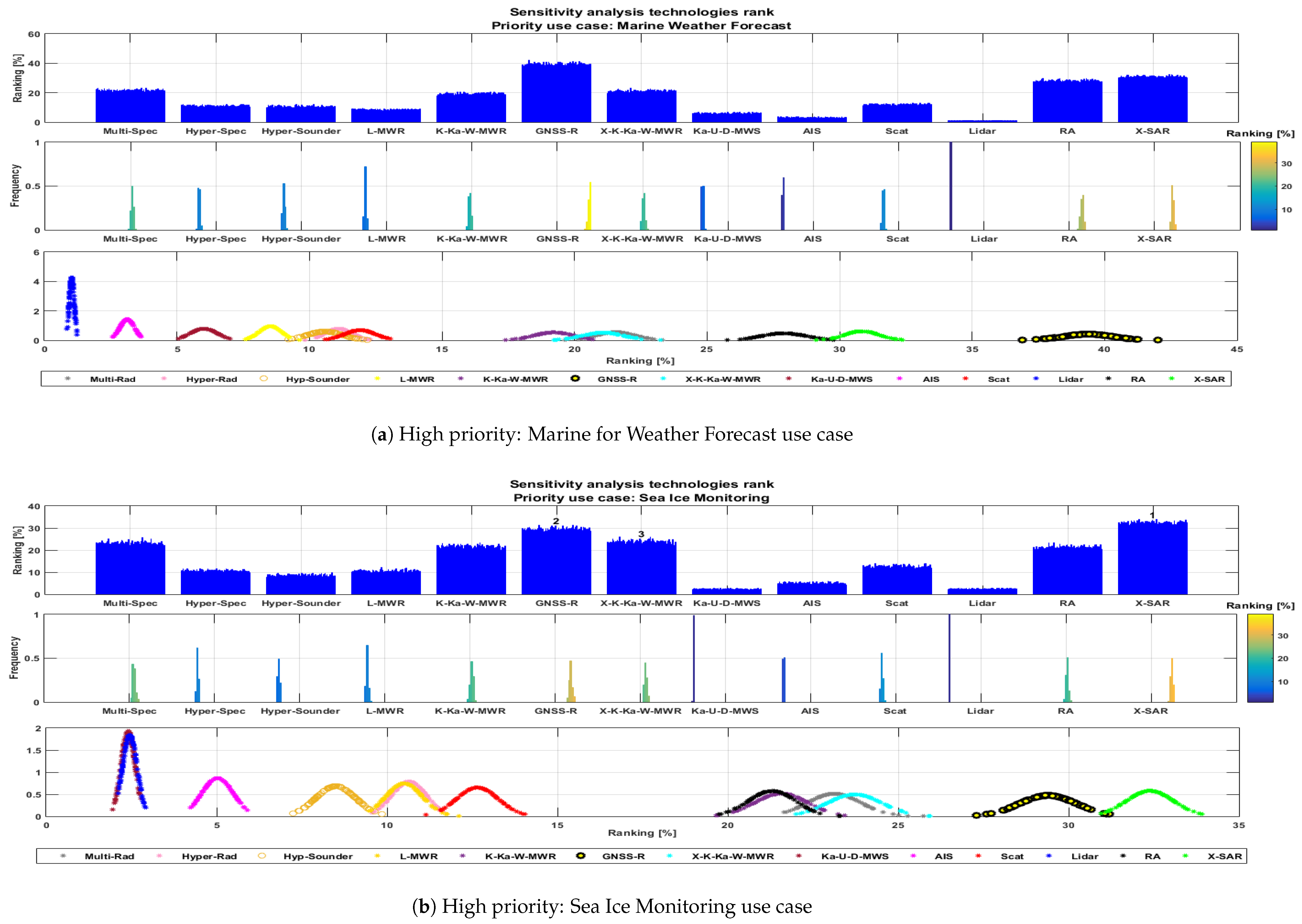
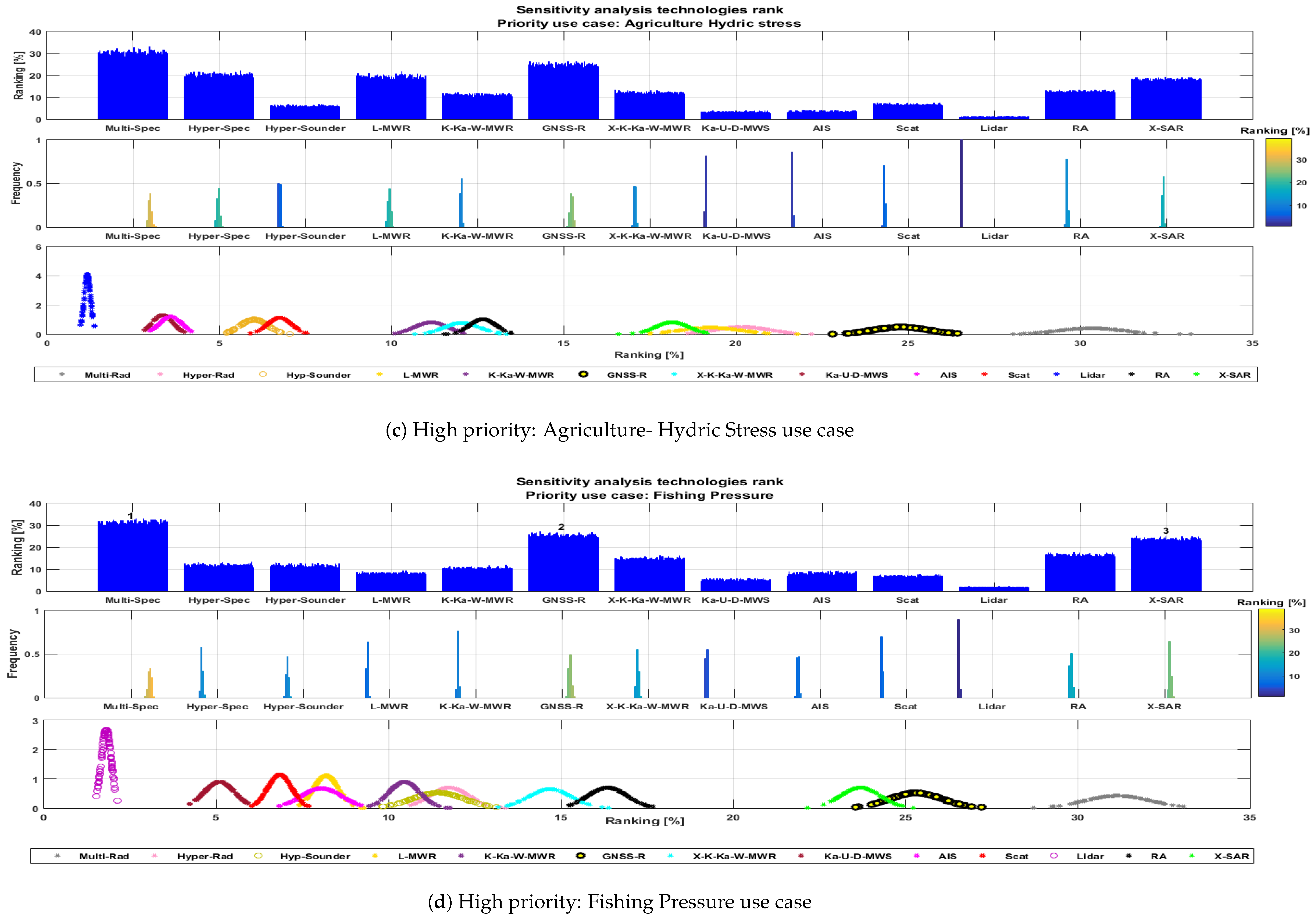
6. Quantitative Method to Identify the Potential Technologies to Cover the Future Copernicus Gaps
- High relevance measurements: ocean surface currents, wind speed over sea surface, dominant wave direction, and significant wave height measurements.
- Medium relevance measurements: sea ice cover, sea ice type, sea surface temperature, and atmospheric pressure over the sea surface.
- Low relevance measurements: Ocean chlorophyll concentration, ocean imagery and weather leaving radiance, CDOM, monitoring system vessels, sea ice extent, sea ice thickness, iceberg tracking, sea ice drift, estimation of crop evapotranspiration, detection of water stress in crops, crop grow and conditions.
- Latency is referred the time to be processed the data to obtain the product.
- Swath is related to the ability of the instrument in order to cover an area, a wide swath indicates minor revisit time.
- Spatial resolution is evaluated for the reference instruments according to the user requirements for each measurement.
- Accuracy is a component of the data quality; it is evaluated according to it being closed to the user requirements for each reference instrument.
- Payload mass is evaluated for each reference instrument, giving priority to the instruments that are best suited to smaller platforms.
- Payload power is related to the power consumption of the payload; it also brings priority to the instruments that are best suited to smaller platforms.
- Data relevance is the potential of the sensor to provide the measure based on sensing constraints (e.g., long time to analyze the data, data limited by cloud cover, and daylight only)
7. Conclusions
Author Contributions
Funding
Conflicts of Interest
Appendix A

| Product | Manufacturer | Total Mass [kg] | Size [cm] | Payload Mass [kg] | Payload Volume | Payload Power [W] | Pointing Control | Pointing Knowledge | Communication Downlink | Propulsion |
|---|---|---|---|---|---|---|---|---|---|---|
| THUNDER (3U) [85] | Space Flight Laboratory | 3.5 | 10 × 10 × 34 | 1 | 1000 cm | 1–2 average | 2 | - | S-band 32 kbps–2 Mbps | Cold Gas |
| Endeavour-3U [18] | Tyvak NanoSatellite Technology Inc. | 5.99 | 30 × 10 × 10 | - | 2U | 12 average, 70 peak | 3 | 25 arcsec | UHF, S-band 10 Mbps | Cold gas |
| GRYPHON (GNB) [85] | Space Flight Laboratory | 7 | 20 × 20 × 20 | 2 | 1700 cm | 3–4 average, 6 peak | 2 | - | S-band 32 kbps–2 Mbps | Cold gas |
| GOMX 1U [98] | GomSpace ApS | 0.725 | 1U | - | 0.4U | 1.33 average | 10 | 5 | UHF, VHF | - |
| GOMX 2U [98] | GomSpace ApS | 1.2 | 2U | - | 1.4U | 2.48 average | 10 | 5 | UHF, VHF | - |
| GOMX 3U [98] | GomSpace ApS | 1.5 | 3U | - | 2.3U | 9.4 average | 10 | 5 | UHF, VHF, optional X-band | - |
| SMALL SAT 6U [12] | Nexeya | 10 | 10 × 22 × 34 | 3 | - | 7 average, 100 peak | - | - | X-band 100 Mb | Available |
| XB-12 [19] | Blue Canyon Technologies LLC | - | 12U | - | 11U | - | 1 arcsec | 0.002 | UHF, S-band, X-band Up to 15 Mbps | Up to 7 thrusters |
| XB-3 [19] | Blue Canyon Technologies LLC | - | 3U | - | 2U | - | - | - | UHF, S-band, X-band Up to 15 Mbps | Up to 7 thrusters |
| XB-6 [19] | Blue Canyon Technologies LLC | - | 6U | - | 5U | - | 1 arcsec | 0.002 | UHF, S-band, X-band Up to 15 Mbps | Up to 7 thrusters |
| MAI-3000 [17] | Maryland Aerospace | 8 | 10 × 10 × 30 | 3 | 1.5U | 12 average | 0.1 or 1.1 | 0.01 or 1 | S-band Up to 2 Mbps, X-band available. | Compatible with existing 3U launch adapters |
| Product | Manufacturer | Total Mass [kg] | Size [cm] | Payload Mass [kg] | Payload Volume | Payload Power Average/Peak [W] | Pointing Control | Pointing Knowledge | Communication | Propulsion |
|---|---|---|---|---|---|---|---|---|---|---|
| MAI-6000 [23] | Maryland Aerospace | 29 | 10 × 20 × 30 | 12 | 4U | 20 | 0.1 | 0.01 | S-band Up to 2 Mbps and X-band available. | Compatible with existing launch dispensers |
| SN-50 [21] | Sierra Nevada Corporation Space Systems | - | - | 50 | 40 × 40 cm | 100 | 0.03 | 0.024 | 3.5 Mbps | Optional green propulsion capability |
| Altair [20] | Millennium Space Systems | - | 30 × 30 × 30 | 50 | - | 90/250 | 20 arcsec | 10 arcsec | S-Band—2 Mbps downlink | - |
| LEOS-30 [95] | Berlin Space Technologies GmbH | 30 | 30 × 30 × 50 | 8 | - | 15/60 | - | - | S-Band—2 Mbps downlink | - |
| LEOS-50 [95] | Berlin Space Technologies GmbH | 60 | 50 × 50 × 30 | 15 | - | 20/140 | - | - | X-band—100 Mbps downlink | - |
| NEMO [85] | Space Flight Laboratory | 15 | 20 × 30 × 40 | 6 | 8000 cm | 45 | 2 | - | S-band 32 kbps–2 Mbps downlink | Cold gas, resistojet, monopropulsion |
| DEFIANT [85] | Space Flight Laboratory | 20–30 | 30 × 30 × 40 | 6–10 | 11,000 cm | 45 | 2 | - | 32 kbps–50 Mbps downlink | Cold gas, resistojet, monopropulsion |
| SMALL SAT 12U [12] | Nexeya | 20 | 22 × 22 × 34 | 30 | - | 12/100 | - | - | S-band 2.5 Mbps downlink, 256 kbps uplink, Optional X-band 100 Mbps downlink | Available |
| SMALL SAT 16U [12] | Nexeya | - | 46 × 22 × 22 | 13 | - | 16/150 | - | - | - | Available |
| SMALL SAT 27U [12] | Nexeya | 40 | 35 × 35 × 34 | 25 | - | 30/200 | - | - | - | Available |
| SSTL-12 [22] | Surrey Satellite Technology Limited | 40–75 | 39 × 39 × 47 | Up 45 | 39 × 39 × 37 cm | 10–30 | 2 | 0.007 | Up to 160 Mbps (X-band) | Available |
| SSTL-X50 Platform [91] | Surrey Satellite Technology Limited | 75 | - | Up 45 | 53 × 43 × 40 cm | 35/85 | 0.07 | 10 arcsec | - | Available |
| SSTL-100 [92] | Surrey Satellite Technology Limited | Up 100 | - | 15 | 32.1 × 30.3 × 24.6 cm 17.9 × 21.6 × 39 cm | 24/48 | 2880 arcsec | 2520 arcsec | Up 80 Mbps | Liquefied Butane Gas |
| XB Microsat [19] | Blue Canyon Technologies LLC | 75 | - | - | 45 × 45 × 80 cm | - | 0.002 | 1 arcsec | UHF, S-band, X-band Up to 150 Mbps downlink | Up to 7 thrusters |
| BCP-50 [96] | Ball Aerospace Commercial Technologies Corp. | 80 | - | 30 | 30 × 30 × 55 cm | 30 e, 100 | 0.03–0.10 | 0.03 | 2 Mbps downlink, | - |
| LEOS-100 [95] | Berlin Space Technologies GmbH | 90 | 60 × 60 × 82.5 | 30 | - | 60/140 | - | - | X-band—100 Mbps downlink | - |
| Product | Manufacturer | Total Mass [kg] | Size [cm] | Payload Mass [kg] | Payload Volume [cm] | Payload Power Average/Peak [W] | Pointing Control | Pointing Knowledge | Payload Data [Downlink] | Propulsion |
|---|---|---|---|---|---|---|---|---|---|---|
| NAUTILUS (NEMO-150) [85] | Space Flight Laboratory | Up 150 | 60 × 60 × 60 | Up 70 | Up 108000 | 50/500 | 2 | - | up to 50 Mbps | Cold gas, resistojet, monopropulsion, Hall thruster. |
| DAUNTLESS [85] | Space Flight Laboratory | Up 500 | 100 × 100 × 100 | Up 250 | Up 500000 | 200/1000 | 2 | - | up to 200 Mbps | Cold gas, resistojet, monopropulsion, Hall thruster. |
| SSTL-150 [92] | Surrey Satellite Technology Limited | Up 150 | 60 × 60 × 30 | 50 | 27.95 × 23.15 × 25.25 | 50 average, 100 peak. | 36 arcsec | 25 arcsec | 80 Mbps | Hot gas Xenon resistojet. |
| SSTL-150 ESPA [86] | Surrey Satellite Technology Limited | - | 60 × 60 × 80 | 65 | 47.5 × 50.5 × 21.1 41 × 54.7 × 24.4 | 120 | 1 arcmin | 2.5 arcsec | 2 Mbps | Available |
| SSTL-300 [92,93] | Surrey Satellite Technology Limited | 368 | 89.9 × 81.5 × 106.1 | 150 | 27.95 × 23.15 × 25.25 | 140 | 360 arcsec | 72 arcsec | S-Band | Hot gas Xenon resistojet |
| TET-1 [111] | Astro- und Feinwerktechnik Adlershof | 120 | 67 × 58 × 88 | 50 | 460 × 460 × 428 | 20 to 80 average, 160 peak for 20 min | 2 arcmin | 10 arcsec | S-band—2.2 Mbps | - |
| BCP-100 [87] | Ball Aerospace Commercial Technologies Corp. | 180 | 60.9 × 71.1 × 96.5 | 70 | 140,000 | 100–200 | 0.03– 0.10 | 0.03 | 2 Mbps for each payload | Green Propellant, Hydrazine options |
| SN- 200 [94] | Sierra Nevada Corporation Space Systems | Up 355 | - | 200 | - | 200 | 0.1 | 0.05 | 274 Mbps (X-band) | Xenon HET (TacSat), 4.5 |
| SSTL-600 [92] | Surrey Satellite Technology Limited | Up 429 | 190 × 140 × 47.6 | 200 | 90.1 × 90.8 × 26 | 386 average, 450 peak | 605 arcsec | 360 arcsec | 500 Mbps (X-band) | Liquefied butane gas |
| Eagle-1M [90] | Northrop Grumman | - | - | >175 | - | 500 average, 1200 peak. | 0.05 | 90 arcsec | - | 200 m/s modular |
| TET-X [13] | OHB | 120 | 58 × 88 × 67 | 50 | 1700 | Max. 80, 160 peak for 25 min | - | 10 arcsec | 100 Mbit/s (X-Band) | Micro propulsion system |
| TET-XL [13] | OHB | 200 | 80 × 84.5 × 80 | 80 | 900 | Max. 150, 460 peak for 25 min. | - | 10 arcsec | 400 Mbit/s (X-Band), or 1.2 Gbit/s (Ka-Band) | Micro propulsion system |
| LEOStar-2 BUS [90] | Northrop Grumman | 150–500 | - | 210–550 | 1,388,000 | up to 2k (optional) | 15 arcsec | 6 arcsec | 2 Mbps (S-Band), 150 Mbps (X-band) | Blowdown monopropellant hydrazine; |
| LEOSTART-500XO [9] | Astrium | 500–1000 | - | 150–600 | - | 250 average, 450 peak | 0.35 | 0.24 deg | 1.6 Mbps (downlink), | Available |
| ELiTeBUS 1000 [10] | Thales Alenia Space | - | - | 350 | 38 × 27.12 × 14.25 | 1000–1500 | 360 arcsec | 22 arcsec | - | Mono-prop (N2H4) |
Appendix B
| Instrument [Mission] | Frequencies Bands [GHz] | Spatial Resolution [km] | Antenna Size [m] | Swath Width [km] | Mass [kg] | Power [W] | Data Rate [kbps] | Orbit Altitude [km] |
|---|---|---|---|---|---|---|---|---|
| Soil Moisture Active and Passive (SMAP) [SMAP] [25,89] | 1.41 | 40 | 6 | 1000 | 356 | 448 | 40,000 | 685 |
| Microwave Imaging Radiometer using Aperture Synthesis (MIRAS) [Soil Moisture and Ocean Salinity (SMOS)] [25,88] | 1.41 | <50 | 4 | 1000 | 355 | 511 | 89 | 755 |
| WindSat (Coriolis) [25] | 6.8, 10.7, 18.7, 23.8, 37 | 39 × 71 to 8 × 13 | 1.83 | 1200 | 341 | 350 | 256 | 838 |
| AMSR (ADEOS-II) [25] | 6.93, 10.65, 18.7, 23.8, 36.5, 50.3, 52.8 and 89 | 3 × 6 to 40 × 70 | 2 | 1600 | 320 | 400 | 130 | 812 |
| AMSR-2 (GCOM) [25] | 6.93, 7.3, 10.65, 18.7, 23.8, 36.5 and 89 | 5 to 50 | 2 | 1450 | 320 | 400 | 130 | 700 |
| AMSR-E (Aqua) [112] | 6.93, 7.3, 10.65, 18.7, 23.8, 36.5 and 89 | 3 × 5 to 35 × 62 | 2.4 | 1450 | 314 | 350 | 874 | 705 |
| Aquarius (SAC-D) [25] | 1.4 GHz | 100 | 2.5 | 390 | 247 | 291 | 5 | 661 |
| MWI (Metop-SG) [25] | 18.7–183.31 (26 channels) | 8 × 13 to 40 × 65 | 0.75 | 1700 | 220 | 250 | 160 | 817 |
| MADRAS (Megha Tropiques) [25] | 18.7, 23.8, 36.5, 89 and 157 | 40 × 60 to 6 × 9 | 0.65 | 1700 | 162 | 153 | 37 | 867 |
| GMI (GPM) [25] | 10.65, 18.7, 23.8, 36.5, 89, 166, 183.31 | 19 × 32 to 4.4 × 7.2 | 1.2 | 850 | 150 | 140 | 25 | 407 |
| TMI (TRMM) [25] | 10.65, 19.35, 21.3, 37, 85.5 | 37 × 63 to 5 × 7 | 0.61 | 790 | 65 | 50 | 8.8 | 402 |
| SSM/I (DMSP) [84] | 19.35, 23.235, 37, 85.5 | 45 × 68 to 11 × 16 | 0.61 | 1400 | 48.5 | 45 | 3.3 | 850 |
| Instrument [mission] | Frequencies [GHz] | Spatial Resolution [km] | Antenna Size [m] | Swath Width [km] | Mass [kg] | Power (W) | Data Rate [kbps] | Orbit Altitude [km] |
|---|---|---|---|---|---|---|---|---|
| ATMS (SNPP, JPSS) [25] | 23.8–183 (22 channels) | 16, 32 and 75 | - | 2600 | 75 | 130 | 30 | 824 |
| AMSU-A (NOAA-15/16/17/18/19, Metop A/B/C and Aqua) [25] | 23 to 89 (15 Channels) | 48 | 0.17 and 0.08 | 2100 | 104 | 99 | 3.4 | 817 |
| Tri-band Microwave Radiometer (MiRaTA) [25,32] | 52–58 175–191 203.8–206.8 (10 channels) | - | 0.1 | - | <4.5 | 6 | 10 | 400 |
| Miniature microwave sounder (EON-MW) [33] | 23/31, 50–60/88, 166/183 (22 channels) | 44, 23, 7.5 | 0.11 | 1000 | 5 | 23 | 50 | 505 |
| Available Instruments | Frequencies & Signals | Spatial Resolution [km] | Swath [km] | Mass [Kg] | Power [W] | Data Rate [kbps] | Orbit Altitude [km] |
|---|---|---|---|---|---|---|---|
| SGR-ReSI (TechDemoSat-1 (TDS-1), CYGNSS) [57] | L1 C/A Code (Options: Galileo E1, GPS L2C, Glonass L1, GPS L5, Galileo E5) | 20–50 | 740 | 1.4 | <12 | 200 | 680 |
| GEROS-ISS (GEROS-ISS) [80] | L1 C/A Code (Options: Galileo E1, GPS L2C, Glonass L1, GPS L5, Galileo E5, and QZSS) | 30 | ∼2000 | 376 | 395 | 1200 | 375–435 |
| FMMPL-2 (FSSCAT) [49] | L1 C/A Code (Options: Galileo E1) | 0.3 | ∼350 | 1.5 | >8.0 | 40 | 500–550 |
| Missions | Satellite Mass [kg] | Size | Power Consumption [W] | Launch Date | Payload |
|---|---|---|---|---|---|
| Triton-2/E-SAIL [97] | 100 | 60 × 60 × 70 cm | 100 | 2018 | AIS |
| Norsat-2/SAT-AIS [97] | 1.5 | 51 × 140 × =168 mm | 5 | 2016 | AIS |
| AISSat [25] | 14 | 1 U | 15 | 2013 | AIS |
| CAT-4 [113] | 9 | 6U | 2 | - | AIS + VIS/NIR camera |
| Canx-6 [25] | 6.5 | 2U | 5.6 | 2008 | AIS |
| AISSat 1 [25] | 6 | - | 0.97 | 2010 | AIS |
| AISSat 2 [25] | 6 | - | 0.97 | 2014 | AIS |
| ZACube-2 [25] | 4 | 3U | - | 2017 | AIS + imager |
| AAUSAT-4 [25] | 0.88 | 1U | 1.15 | 2016 | AIS |
| Instrument (Mission) | Classification | Wavelength [m] | Aperture Size [m] | Spatial Resolution [km] | Swath Width [km] | Mass [kg] | Power [W] | Data Rate [Mbps] | Orbit Altitude [km] |
|---|---|---|---|---|---|---|---|---|---|
| MetImage (MetOp-SG) [25] | Radiometer/ Multispectral resolution | [0.443–13.345] 20 spectral channels | 0.17 | 0.25 to 0.5 or 1 | 2670 | 296 | 465 | 18 | 817 |
| VIIRS (NOAA-20) [25] | Radiometer/ Multispectral resolution | [0.4–12.5] 22 spectral channels | 0.184 | 0.375 to 0.75 | 3000 | 275 | 240 | 5.9 | 825 |
| Modis (Terra/Aqua) [25] | Radiometer/ Multispectral resolution | [0.4–14] 36 spectral channels | 0.178 | 0.25–1 | 2330 | 229 | 162.5 | 6.1 | 705 |
| SLSTR (Sentinel-3) [24,25] | Radiometer/ Multispectral resolution | [0.545–12.5] 11 spectral channels | - | 0.5–1.0 | 1400 | 140 | 100 | 64 | 814.5 |
| OLCI (Sentinel-3) [25] | Radiometer/ Multispectral resolution | [0.55–10.85] 21 spectral channels | - | 0.3 | 1270 | 150 | 124 | 5 | 814.5 |
| AATSR (Envisat) [25] | Radiometer/ Multispectral resolution | [0.4–15] 7 spectral channels | - | 1 | 500 | 101 | 100 | 0.625 | 774 |
| VIRS (TRMM) [25] | Radiometer/ Multispectral resolution | [0.58–12.05] | - | 2 | 833 | 34.5 | 40 | 0.05 | 402 |
| AVHRR/3 (Metop/ NOAA) [25,61] | Radiometer/ Multispectral resolution | [0.58–12.5] 6 spectral channels | 0.21 × 0.295 | 1.1 | 2900 | 33 | 27 | 0.621 | 850 |
| Naomi (SPOT-6/7) [25] | Radiometer/ Multispectral resolution | [0.45–0.89] 5 spectral channels | - | 0.08 | 25 | 18.5 | - | 60 | 695 |
| CHRIS (PROBA-1) [25] | Imager Spectrometer/ Hyperspectral resolution | [0.4–1.05] 63 spectral channels | 0.12 | 0.036 | 14 | 14 | 8 | 1 | 615 |
| COMIS (STSat-3) [25] | Imager Radiometer/ Hyperspectral resolution | [0.4–1.05] 64 spectral channels | - | 30 or 60 | 15 or 30 | 4.3 | 5 | - | 700 |
| HyperScout/ FSSCAT, (3CAT 5/B) [49] | Imager/ Hyperspectral resolution | [0.4–1.0] 45 spectral bands | 0.1 | 0.04 | 164 | 1.1 | 11 | - | 300 |
| CIRC (ALOS-2) [25] | Infrared radiometer | [8–12] Single TIR channel | 0.08 | 200 | 128 | 3 | <20 | - | 640 |
| Instrument (Mission) | Classification | Wavelength [m] | Aperture Size [m] | Spatial Resolution [km] | Swath Width [km] | Mass [kg] | Power [W] | Data Rate [Mbps] | Orbit Altitude [km] |
|---|---|---|---|---|---|---|---|---|---|
| IASI (MetOp) [25] | Fourier Transform spectrometer b Radiometer/ Hyperspectral resolution | [3.62–15.5] 8461 spectral samples | 1.1 | 25, 1–30 | 2052 | 236 | 210 | 1.5 | 827 |
| AIRS (Aqua) [25] | Infrared sounder/ Hyperspectral resolution | [0.4–15.4] spectral channel >2300 | 0.219 | 13.5, 1 | 1650 | 177 | 220 | 1.27 | 705 |
| CrIS (JPSS) [25] | Infrared Sounder/ Hyperspectral resolution | [3.92–15.38] 1345 spectral channels | 0.8 | 14 | 2200 | 152 | 124 | 1.5 | 824 |
| HIRS/4 (MetOp, NOAA) [25] | Infrared sounder/ Multispectral resolution | [0.69–14.95] 20 spectral channels | 0.15 | 10 | 2160 | 35 | 24 | 0.003 | 850 |
| EON-IR CIRAS [25,62] | Infrared Sounder/ Hyperspectral resolution | [4.08–5.13] 625 channels | 0.15 | 3, 13.5 | 2200 | 2.5 | 15 | 2 | 450–600 |
| Instrument/Mission | Frequency [GHz] | Antenna Size [m] | Spatial Resolution [km] | Mass [kg] | Power [W] | Data Rate [kbps] | Orbit Altitude [km] |
|---|---|---|---|---|---|---|---|
| Altika/SARAL [25] | 23.8, 36.5, 35.75 | 1 | 10 | 40 | 85 | 43 | 800 |
| SWIM/CFOSAT [25] | 13.58 | 0.9 | - | - | 120 | 50 | 519 |
| Altimeter/SWOT [24] | 5.3, 13.58 | 1.2 | 25 | 70 | 78 | 22.5 | 891 |
| Karin*/SWOT [24] | 35.75 | 5 × 0.25 | 0.05 1 | 300 | 1100 | 320,000 | 891 |
| RA-2/Envisat [24,25] | 3.2, 13.6 | 1.5 | 20 | 110 | 161 | 100 | 774 |
| SSALT/TOPEX- Poseidon [24,25] | 13.65 | 1.5 | 25 | 24 | 49 | - | 1336 |
| Instrument (Mission) | Frequencies [GHz] | Spatial Resolution [km] | Swath Width [km] | Mass [kg] | Power [W] | Data Rate [kbps] | Orbit Altitude [km] |
|---|---|---|---|---|---|---|---|
| ASCAT (Metop) [25] | 5.255 | 50, 25 and 12.5 | 550 | 260 | 215 | 42 | 817 |
| RapidScat (ISS RapidScat) [24] | 13.4 | 50, 25 and 12.5 | 900 | 200 | 220 | 40 | 407 |
| SCA (Metop-SG-B1/B2/B3) [25] | 5.3 | 17–25 | 550 | 600 | 540 | 5000 | 817 |
| SCAT (CFOSAT) [25,82] | 13.256 | 50, 10 | >1000 | <70 | <200 | 220 | 500 |
| WindRAD (FY-3E/3H) [25] | 5.3 and 13.265 | 20 (C-band), and 10 (Ku-band) | 1200 | - | 265 | - | 836 |
| Instrument/Mission | Frequency [GHz] | Antenna Size [m] | Spatial Resolution [km] | Mass [kg] | Power [W] | Data Rate [kbps] | Orbit Altitude [km] |
|---|---|---|---|---|---|---|---|
| SIRAL/Cryosat-2 [24,25] | 13.56 | 1.2 | 15 0.25 | 70 | 149 | 24,000 | 717 |
| SRAL/Sentinel-3 [24,25] | 5.3, 13.58 | 1.2 | 20 0.3 | 60 | 90 | 12,000 | 810 |
| Poseidon-4/ Sentinel-6 [24] | 5.3, 13.58 | - | 20 0.3 | 60 | 90 | 12,000 | 1336 |
| Instrument/ Mission | Frequency [GHz] | Spatial Resolution [m] @ Swath [km] | Mass [kg] | Power [W] | Data Rate [Mbps] | Orbit Altitude [km] |
|---|---|---|---|---|---|---|
| L-band SAR/SAOCOM-2 [24] | 1.275 | 10–100 @ 30–320 | 1500 | - | 300 | 620 |
| X-Band SAR/TSX-NG [24] | 9.65 | 1–16 @ 10–100 | 1230 | 2400 | 680 | 515 |
| SAR/RISAT-1/1A/2 [24] | 5.35 | 1–50 @ 10–220 | 950 | 3100 | 1478 | 546 |
| C-Band SAR/Sentinel-1 [24] | 5.405 | 9–50 @ 80–400 | 880 | 4400 | 600 | 693 |
| SAR (CSA)/RADARSAT [24] | 5.405 | 16–100 @ 20–500 | 705 | 1650 | 105 | 798 |
| SAR RCM/RCM [24] | 5.4 | 3–100 @ 20–500 | 600 | 1270 | - | 592 |
| COSI/KOMPSAT-5 [24] | 9.66 | 1–20 @ 5–100 | 520 | 600 | 310 | 550 |
| Severjanin-M/Meteor-M N2 [25,83] | 9.623 | 400–1000 @ 600 | 150 | 1000 | 10 | 830 |
| Type of Lidar | Instrument/ Mission | Wavelength [nm] | Mass [kg] | Power [W] | Data Rate [kbps] | Vertical Spatial Resolution [m] | Swath [m] | Orbit Altitude [km] |
|---|---|---|---|---|---|---|---|---|
| Doppler Lidar | ALADIN/ ADM-Aeolus [25] | 355 | 500 | 840 | 11 | 250 | 50,000 | 405 |
| Backscatter LIDAR | ATLID/ EarthCare [25] | 354.8 | 230 | 320 | 820 | 100 | 100 | 394 |
| CALIOP/ CALIPSO [25] | 532, 1064 | 156 | 124 | 332 | 30 | 333 | 705 | |
| CATS/ ISS CATS [25] | 355, 532, 1064 | 494 | 1000 | 2000 | 30 | 3500 | 407 | |
| LIDAR Altimeter | VCL/ DESDynl [24] | 1064 | 225 | 336 | 800 | 1 | 25,000 | 400 |
| GEDI-Lidar/ ISS GEDI [24] | 1064.5 | 230 | 516 | 2100 | 25 | 7000 | 407 | |
| ATLAS/ ICESat-2 [24] | 1064 | 298 | 300 | 0.45 | 0.1 | 170 | 478 | |
| GLAS/ ICESat [24] | 532, 1064 | 298 | 300 | 0.45 | 0.1 | 170 | 600 | |
| Differential Absorption Lidar (DIAL) | IPDA LIDAR/ MERLIN [24,25] | 1645 | 32.5 | 57 | 150,000 | 100 | 0.1 | 506 |
References
- Earth Explorer Missions. Available online: https://www.esa.int/Our_Activities/Observing_the_Earth/Earth_Explorers_an_overview (accessed on 19 December 2018).
- European Space Agency: Two New Earth Explorer Concepts to Understand Our Rapidly Changing World. Available online: https://www.esa.int/Our_Activities/Observing_the_Earth/Two_new_Earth_Explorer_concepts_to_understand_our_rapidly_changing_world (accessed on 19 December 2018).
- ESA Status Report. Available online: http://www.wmo.int/pages/prog/sat/meetings/ET-SAT-11/documents/ET-SAT-11_Doc_3.4_ESA%20EOP%20%20Status%20Report-%204%20April%202017.pdf (accessed on 19 December 2018).
- Study to Examine the Socio-Economic Impact of Copernicus in the EU—Report on the Socio-Economic Impact of the Copernicus Programme. Available online: https://publications.europa.eu/en/publication-detail/-/publication/62e30ab0-aa54-11e6-aab7-01aa75ed71a1/language-en/format-PDF/source-search (accessed on 17 December 2018).
- Matevosyan, H.; Lluch, I.; Poghosyan, A.; Golkar, A. A Value-Chain Analysis for the Copernicus Earth Observation Infrastructure Evolution: A Knowledgebase of Users, Needs, Services, and Products. IEEE Geosci. Remote Sens. Mag. 2017, 5, 19–35. [Google Scholar] [CrossRef]
- Lancheros, E.; Camps, A.; Park, H.; Sicard, P.; Mangin, A.; Matevosvan, I.; Lluch, I. Gaps Analysis and Requirements Specification for the Evolution of Copernicus System for Polar Regions Monitoring: Addressing the Challenges in the Horizon 2020–2030. Remote Sens. 2018, 10, 1098. [Google Scholar] [CrossRef]
- European Space Agency: Sentinels Satellites. Available online: http://www.esa.int/Our_Activities/Observing_the_Earth/Copernicus/Overview4 (accessed on 17 December 2018).
- European Space Agency: Copernicus Contributing Missions. Available online: https://spacedata.copernicus.eu/web/cscda/missions (accessed on 17 December 2018).
- Dribault, L.; Durteste, C.; Salvatori, A. LeoStart: Lessons Learnt and Perspectives. Small Satellite Conference, 2013. Available online: https://digitalcommons.usu.edu/smallsat/2000/All2000/22/ (accessed on 17 December 2018).
- Thales Alenia Space: ELiTeBUS™1000 Platform. Available online: https://www.thalesgroup.com/sites/default/files/asset/document/20161212_pr_elitebus_rsdo_en.pdf (accessed on 7 June 2018).
- Bowen, J.; Tsuda, A.; Abel, J.; Villa, M. CubeSat Proximity Operations Demonstration (CPOD) mission update. In Proceedings of the IEEE Aerospace Conference Proceedings, Big Sky, MT, USA, 7–14 March 2015. [Google Scholar]
- Nexeya: Small Satellites. Available online: http://www.nexeya.com/solutions/space-systems/nano-satellites/ (accessed on 16 January 2019).
- OHB System AG: TET the Small Satellites Series. Available online: https://www.ohb-system.de/tl_files/system/images/mediathek/downloads/pdf/OHB_Messe_TET_2014_web.pdf (accessed on 7 June 2018).
- Small Geostationary Satellite (SGEO) / Telecommunications & Integrated Applications / Our Activities / ESA. Available online: http://www.esa.int/Our_Activities/Telecommunications_Integrated_Applications/Small_Geostationary_Satellite_SGEO (accessed on 7 June 2018).
- OHB System AG: SmallGeo. Available online: https://www.ohb-system.de/small-geo-luxor-english.html (accessed on 7 June 2018).
- Sun, D.W.; Ellmers, F.; Winkler, A.; Schuff, H.; Sansegundo Chamarro, M.J. European small geostationary communications satellites. Acta Astron. 2011, 68, 802–810. [Google Scholar] [CrossRef]
- Maryland Aerospace: Platform Products—MAI-3000—3U CubeSat. Available online: https://www.adcolemai.com/3u-cubesat-mai-3000 (accessed on 7 June 2018).
- Macgillivray, S. Tyvak Nano-Satellite Systems LLC ™ Endeavour: The Product Suite for Next Generation CubeSat Mission. Available online: http://mstl.atl.calpoly.edu/~bklofas/Presentations/SummerWorkshop2012/MacGillivray_Endevour.pdf (accessed on 12 June 2018).
- Blue Canyon Technologies: Spacecraft Buses, Systems & Solutions—XB Spacecraft Buses. Available online: http://bluecanyontech.com/wp-content/uploads/2018/01/DataSheet_XBSpacecraft_11_F.pdf (accessed on 8 June 2018).
- Millennium Space Systems—Altair Platforms. Available online: http://www.millennium-space.com/platforms.html#altair (accessed on 8 June 2018).
- Sierra Nevada Corporation (SNC): Spacecraft Systems—SN-50 Nanosat. Available online: http://mediakit.sncorp.com/mediastore/mediakit/sncspace/146/snc’s%20spacecraft%20systems%20overview%20brochure_sn-50_low%20res.pdf (accessed on 8 June 2018).
- Surrey Satellite Technology Ltd.: SSTL-12 Platform—Mission Configurations. Available online: http://www.sst-us.com/downloads/datasheets/us_platforms_stl-12.pdf (accessed on 7 June 2018).
- Maryland Aerospace: Platform Products—MAI-6000—6U CubeSat. Available online: https://www.adcolemai.com/6u-cubesat-mai-6000 (accessed on 7 June 2018).
- World Meteorological Organization: Observing Systems Capability Analysis and Review Tool—Space-Based Capabilities. Available online: https://www.wmo-sat.info/oscar/spacecapabilities (accessed on 7 June 2018).
- Earth Observation Portal Directory: Satellite Missions Database. Available online: https://directory.eoportal.org/web/eoportal/satellite-missions (accessed on 7 June 2018).
- Zhang, L.; Shi, H.; Wang, Z.; Yu, H.; Yin, X.; Liao, Q. Comparison of Wind Speeds from Spaceborne Microwave Radiometers with In Situ Observations and ECMWF Data over the Global Ocean. Remote Sens. 2018, 10, 425. [Google Scholar] [CrossRef]
- Tauro, C.B.; Hejazin, Y.; Jacob, M.M.; Jones, W.L. An Algorithm for Sea Surface Wind Speed from SAC-D/Aquarius Microwave Radiometer. IEEE J. Sel. Top. Appl. Earth Obs. Remote Sens. 2015, 8, 5485–5490. [Google Scholar] [CrossRef]
- Kaleschke, L.; Tian-Kunze, X.; Maaß, N.; Mäkynen, M.; Drusch, M. Sea ice thickness retrieval from SMOS brightness temperatures during the Arctic freeze-up period. Geophys. Res. Lett. 2012, 39. [Google Scholar] [CrossRef]
- Ricker, R.; Hendricks, S.; Kaleschke, L.; Tian-Kunze, X.; King, J.; Haas, C. A weekly Arctic sea-ice thickness data record from merged CryoSat-2 and SMOS satellite data. Cryosphere 2017, 11, 1607–1623. [Google Scholar] [CrossRef]
- Ivanova, N.; Pedersen, L.T.; Tonboe, R.T.; Kern, S.; Heygster, G.; Lavergne, T.; Sørensen, A.; Saldo, R.; Dybkjær, G.; Brucker, L.; et al. Inter-comparison and evaluation of sea ice algorithms: Towards further identification of challenges and optimal approach using passive microwave observations. Cryosphere 2015. [Google Scholar] [CrossRef]
- Araguz, C.; Llaveria, D.; Lancheros, E.; Bou-Balust, E.; Camps, A.; Alarcón, E.; Lluch, I.; Matevosyan, H.; Golkar, A.; Tonetti, S.; et al. Architectural optimization results for a network of Earth-observing satellite nodes. In Proceedings of the 5th Federated and Fractionated Satellite Systems Workshop, Toulouse, France, 2–3 November 2017. [Google Scholar]
- Blackwell, W.J. New Small Satellite Capabilities for Microwave Atmospheric Remote Sensing. In Proceedings of the IEEE MTT-S International Microwave Symposium, Honolulu, HI, USA, 4–9 June 2017. [Google Scholar]
- Blackwell, W.J.; Pereira, J. New Small Satellite Capabilities for Microwave Atmospheric Remote Sensing: The Earth Observing Nanosatellite-Microwave (EON-MW); American Meteorological Society: Boston, MA, USA, 2016. [Google Scholar]
- Carreno-Luengo, H.; Camps, A.; Perez-Ramos, I.; Forte, G.; Onrubia, R.; Diez, R. 3Cat-2: A P(Y) and C/A GNSS-R experimental nano-satellite mission. In Proceedings of the International Geoscience and Remote Sensing Symposium (IGARSS), Melbourne, VIC, Australia, 21–26 July 2013; pp. 843–846. [Google Scholar] [CrossRef]
- Semmling, A.M.; Beckheinrich, J.; Wickert, J.; Beyerle, G.; Schön, S.; Fabra, F.; Pflug, H.; He, K.; Schwabe, J.; Scheinert, M. Sea surface topography retrieved from GNSS reflectometry phase data of the GEOHALO flight mission. Geophys. Res. Lett. 2014. [Google Scholar] [CrossRef]
- Morris, M.; Ruf, C.S. Determining tropical cyclone surface wind speed structure and intensity with the CYGNSS satellite constellation. J. Appl. Meteorol. Climatol. 2017. [Google Scholar] [CrossRef]
- Clarizia, M.P.; Gommenginger, C.P.; Gleason, S.T.; Srokosz, M.A.; Galdi, C.; Di Bisceglie, M. Analysis of GNSS-R delay-Doppler maps from the UK-DMC satellite over the ocean. Geophys. Res. Lett. 2009. [Google Scholar] [CrossRef]
- Mashburn, J.; Axelrad, P.; Lowe, S.T.; Larson, K.M. Global Ocean Altimetry with GNSS Reflections from TechDemoSat-1. IEEE Trans. Geosci. Remote Sens. 2018, 56, 4088–4097. [Google Scholar] [CrossRef]
- Clarizia, M.P.; Ruf, C.S.; Jales, P.; Gommenginger, C. Spaceborne GNSS-R minimum variance wind speed estimator. IEEE Trans. Geosci. Remote Sens. 2014, 52, 6829–6843. [Google Scholar] [CrossRef]
- Wang, F.; Yang, D.; Zhang, B.; Li, W. Waveform-based spaceborne GNSS-R wind speed observation: Demonstration and analysis using UK TechDemoSat-1 data. Adv. Space Res. 2018, 61, 1573–1587. [Google Scholar] [CrossRef]
- Camps, A.; Park, H.; Pablos, M.; Foti, G.; Gommenginger, C.P.; Liu, P.W.; Judge, J. Sensitivity of GNSS-R Spaceborne Observations to Soil Moisture and Vegetation. IEEE J. Sel. Top. Appl. Earth Obs. Remote Sens. 2016, 9, 4730–4742. [Google Scholar] [CrossRef]
- Chew, C.; Shah, R.; Zuffada, C.; Hajj, G.; Masters, D.; Mannucci, A.J. Demonstrating soil moisture remote sensing with observations from the UK TechDemoSat-1 satellite mission. Geophys. Res. Lett. 2016, 43, 3317–3324. [Google Scholar] [CrossRef]
- Alonso-Arroyo, A.; Camps, A.; Aguasca, A.; Forte, G.; Monerris, A.; Rudiger, C.; Walker, J.P.; Park, H.; Pascual, D.; Onrubia, R. Improving the accuracy of soil moisture retrievals using the phase difference of the dual-polarization GNSS-R interference patterns. IEEE Geosci. Remote Sens. Lett. 2014, 11, 2090–2094. [Google Scholar] [CrossRef]
- Rodriguez-Alvarez, N.; Bosch-Lluis, X.; Camps, A.; Aguasca, A.; Vall-Llossera, M.; Valencia, E.; Ramos-Perez, I.; Park, H. Review of crop growth and soil moisture monitoring from a ground-based instrument implementing the Interference Pattern GNSS-R Technique. Radio Sci. 2011, 46. [Google Scholar] [CrossRef]
- Larson, K.M.; Braun, J.J.; Small, E.E.; Zavorotny, V.U.; Gutmann, E.D.; Bilich, A.L. GPS Multipath and Its Relation to Near-Surface Soil Moisture Content. IEEE J. Sel. Top. Appl. Earth Obs. Remote Sens. 2010, 3, 91–99. [Google Scholar] [CrossRef]
- Li, W.; Cardellach, E.; Fabra, F.; Rius, A.; Ribó, S.; Martín-Neira, M. First spaceborne phase altimetry over sea ice using TechDemoSat-1 GNSS-R signals. Geophys. Res. Lett. 2017, 44, 8369–8376. [Google Scholar] [CrossRef]
- Alonso-Arroyo, A.; Zavorotny, V.U.; Camps, A. Sea Ice Detection Using U.K. TDS-1 GNSS-R Data. IEEE Trans. Geosci. Remote Sens. 2017, 55, 4989–5001. [Google Scholar] [CrossRef]
- Foti, G.; Gommenginger, C.; Jales, P.; Unwin, M.; Shaw, A.; Robertson, C.; Rosellõ, J. Spaceborne GNSS reflectometry for ocean winds: First results from the UK TechDemoSat-1 mission. Geophys. Res. Lett. 2015, 42, 5435–5441. [Google Scholar] [CrossRef]
- Copernicus Masters: FSSCat—Towards Federated EO Systems. Available online: https://www.copernicus-masters.com/winner/ffscat-towards-federated-eo-systems/ (accessed on 9 June 2018).
- Castellví, J.; Camps, A.; Corbera, J.; Alamús, R. 3Cat-3/MOTS nanosatellite mission for optical multispectral and GNSS-R earth observation: Concept and analysis. Sensors 2018, 18, 140. [Google Scholar] [CrossRef] [PubMed]
- Park, H.; Pascual, D.; Camps, A.; Martin, F.; Alonso-Arroyo, A.; Carreno-Luengo, H. Analysis of spaceborne GNSS-R delay-doppler tracking. IEEE J. Sel. Top. Appl. Earth Obs. Remote Sens. 2014. [Google Scholar] [CrossRef]
- Martín-Neira, M.; D’Addio, S.; Buck, C.; Floury, N.; Prieto-Cerdeira, R. The PARIS ocean altimeter in-Orbit demonstrator. IEEE Trans. Geosci. Remote Sens. 2011, 49, 2209–2237. [Google Scholar] [CrossRef]
- Camps, A.; Park, H.; Valencia I Domenech, E.; Pascual, D.; Martin, F.; Rius, A.; Ribo, S.; Benito, J.; Andres-Beivide, A.; Saameno, P.; et al. Optimization and performance analysis of interferometric GNSS-R altimeters: Application to the PARIS IoD mission. IEEE J. Sel. Top. Appl. Earth Obs. Remote Sens. 2014, 7, 1436–1451. [Google Scholar] [CrossRef]
- Martin-Neira, M. A Passive Reflectometry and Interferometry System(PARIS)- Application to ocean altimetry. ESA J. 1993, 17, 331–355. [Google Scholar]
- Camps, A.; Park, H.; Sekulic, I.; Rius, J.M. GNSS-R altimetry performance analysis for the GEROS experiment on board the international space station. Sensors 2017, 17, 1583. [Google Scholar] [CrossRef]
- Ribo, S.; Arco, J.C.; Oliveras, S.; Cardellach, E.; Rius, A.; Buck, C. Experimental results of an x-band PARIS receiver using digital satellite TV opportunity signals scattered on the sea surface. IEEE Trans. Geosci. Remote Sens. 2014, 52, 5704–5711. [Google Scholar] [CrossRef]
- Surrey Satellite Technology: SGR-ReSI. Available online: http://www.sst-us.com/getfile/e4b5fba3-8d9a-499d-8e50-568ffa156bcd (accessed on 9 June 2018).
- GOMSpace. GOMspace: Ship Tracking with Space based AIS Receiver. Available online: https://gomspace.com/Shop/payloads/ship-tracking.aspx (accessed on 18 September 2018).
- Cooley, S.W.; Smith, L.C.; Stepan, L.; Mascaro, J. Tracking dynamic northern surface water changes with high-frequency planet CubeSat imagery. Remote Sens. 2017, 9, 1306. [Google Scholar] [CrossRef]
- Selva, D.; Krejci, D. A survey and assessment of the capabilities of Cubesats for Earth observation. Acta Astron. 2012, 74, 50–68. [Google Scholar] [CrossRef]
- Polar Operational Envoromental Satellites (POES): AVHRR/3. Available online: https://poes.gsfc.nasa.gov/avhrr3.html (accessed on 12 June 2018).
- Pagano, T.; Abesamis, C.; Andrade, A.; Aumann, H.; Gunapala, S.; Heneghan, C.; Jarnot, R.; Johnson, D.; Lamborn, A.; Maruyama, Y.; et al. Design and development of the CubeSat Infrared Atmospheric Sounder (CIRAS). SPIE In. Soc. Opt. Eng. 2017, 10402. [Google Scholar] [CrossRef]
- Dawson, G.J.; Bamber, J.L. Antarctic Grounding Line Mapping From CryoSat-2 Radar Altimetry. Geophys. Res. Lett. 2017. [Google Scholar] [CrossRef]
- Tournadre, J.; Bouhier, N.; Boy, F.; Dinardo, S. Detection of iceberg using Delay Doppler and interferometric Cryosat-2 altimeter data. Remote Sens. Environ. 2018. [Google Scholar] [CrossRef]
- Richard, J.; Enjolras, V.; Rys, L.; Vallon, J.; Nann, I.; Escudier, P. Space Altimetry from Nano-Satellites: Payload Feasibility, Missions and System Performances. In Proceedings of the IGARSS 2008, 2008 IEEE International Geoscience and Remote Sensing Symposium, Boston, MA, USA, 7–11 July 2008. [Google Scholar]
- Vogelzang, J.; Stoffelen, A. Scatterometer wind vector products for application in meteorology and oceanography. J. Sea Res. 2012, 74, 16–25. [Google Scholar] [CrossRef]
- Reimer, A.C.; Melzer, B.T.; Kidd, C.R.; Wagner, D.W. Validation of the enhanced resolution ERS-2 scatterometer soil moisture product. In Proceedings of the International Geoscience and Remote Sensing Symposium (IGARSS), Munich, Germany, 22–27 July 2012; pp. 1208–1211. [Google Scholar] [CrossRef]
- Brakke, T.W.; Kanemasu, E.T.; Steiner, J.L.; Ulaby, F.T.; Wilson, E. Microwave radar response to canopy moisture, leaf-area index, and dry weight of wheat, corn, and sorghum. Remote Sens. Environ. 1981, 11, 207–220. [Google Scholar] [CrossRef]
- Foster, J.L.; Hall, D.K.; Eylander, J.B.; Kim, E.D.; Riggs, G.A.; Tedesco, M.; Nghiem, S.V.; Kelly, R.E.J.; Choudhury, B.; Reichle, R. Blended Visible, Passive Microwave and Scatterometer Global Snow Products. In Proceedings of the 64th Eastern Snow Conference, St. John’s, NL, Canada, 29 May–1 June 2007; pp. 27–36. [Google Scholar]
- Belmonte Rivas, M.; Verspeek, J.; Verhoef, A.; Stoffelen, A. Bayesian sea ice detection with the advanced scatterometer ASCAT. IEEE Trans. Geosci. Remote Sens. 2012, 50, 2649–2657. [Google Scholar] [CrossRef]
- Alarcon, E.; Sanchez, A.A.; Araguz, C.; Barrot, G.; Bou-Balust, E.; Camps, A.; Cornara, S.; Cote, J.; Pena, A.G.; Lancheros, E.; et al. Design and optimization of a polar satellite mission to complement the copernicus system. IEEE Access 2018. [Google Scholar] [CrossRef]
- Gebert, N.; Domínguez, B.C.; Davidson, M.W.J.; Martin, M.D.; Silvestrin, P. SAOCOM-CS—A passive companion to SAOCOM for single-pass L-band SAR interferometry. In Proceedings of the European Conference on Synthetic Aperture Radar, Berlin, Germany, 3–5 June 2014; pp. 1251–1254. [Google Scholar]
- Surrey Satellite Technology Ltd.: NovaSAR-S—The Small Satellite Approack to Synthetic Aperture Radar. Available online: https://www.sstl.co.uk/Downloads/Brochures/115184-SSTL-NovaSAR-Brochure-high-res-no-trims (accessed on 7 June 2018).
- ICEYE Satellite Missions. Available online: https://www.iceye.com/resources/satellite-missions (accessed on 4 October 2018).
- Slobbe, D.C.; Lindenbergh, R.C.; Ditmar, P. Estimation of volume change rates of Greenland’s ice sheet from ICESat data using overlapping footprints. Remote Sens. Environ. 2008. [Google Scholar] [CrossRef]
- Lefsky, M.A.; Harding, D.J.; Keller, M.; Cohen, W.B.; Carabajal, C.C.; Del Bom Espirito-Santo, F.; Hunter, M.O.; de Oliveira, R. Estimates of forest canopy height and aboveground biomass using ICESat. Geophys. Res. Lett. 2005. [Google Scholar] [CrossRef]
- Winker, D.M.; Pelon, J.; Coakley, J.A.; Ackerman, S.A.; Charlson, R.J.; Colarco, P.R.; Flamant, P.; Fu, Q.; Hoff, R.M.; Kittaka, C.; et al. The Calipso Mission: A Global 3D View of Aerosols and Clouds. Bull. Am. Meteorol. Soc. 2010. [Google Scholar] [CrossRef]
- Illingworth, A.J.; Barker, H.W.; Beljaars, A.; Ceccaldi, M.; Chepfer, H.; Clerbaux, N.; Cole, J.; Delanoë, J.; Domenech, C.; Donovan, D.P.; et al. The earthcare satellite: The next step forward in global measurements of clouds, aerosols, precipitation, and radiation. Bull. Am. Meteorol. Soc. 2015. [Google Scholar] [CrossRef]
- Stoffelen, A.; Marseille, G.J.; Bouttier, F.; Vasiljevic, D.; de Haan, S.; Cardinali, C. ADM-Aeolus Doppler wind lidar Observing System Simulation Experiment. Q. J. R. Meteorol. Soc. 2006. [Google Scholar] [CrossRef]
- Wickert, J.; Cardellach, E.; Martin-Neira, M.; Bandeiras, J.; Bertino, L.; Andersen, O.B.; Camps, A.; Catarino, N.; Chapron, B.; Fabra, F.; et al. GEROS-ISS: GNSS REflectometry, Radio Occultation, and Scatterometry Onboard the International Space Station. IEEE J. Sel. Top. Appl. Earth Obs. Remote Sens. 2016, 9, 4552–4581. [Google Scholar] [CrossRef]
- Camps, A.J.; Swift, C.T. A two-dimensional Doppler-radiometer for earth observation. IEEE Trans. Geosci. Remote Sens. 2001. [Google Scholar] [CrossRef]
- Hauser, D.; Tison, C.; Amiot, T.; Delaye, L.; Mouche, A.; Guitton, G.; Aouf, L.; Castillan, P. CFOSAT: A new Chinese-French satellite for joint observations of ocean wind vector and directional spectra of ocean waves. Remote Sens. 2016, 98780T, 1–20. [Google Scholar] [CrossRef]
- Vnotchenko, S.; Dostovalov, M.; Dudukin, V.; Kovalenko, A.; Musinyants, T.; Riman, V.; Selyanin, A.; Smirnov, S.; Telichev, A.; Chernishov, V.; et al. Wide-swath spaceborne SAR system “Severyanin-M” for remote sensing: First results. In Proceedings of the 9th European Conference on Synthetic Aperture Radar, Nuremberg, Germany, 23–26 April 2012; pp. 422–425. [Google Scholar]
- Special Sensor Microwave Imager (SSM/I) | National Snow and Ice Data Center. Available online: https://nsidc.org/data/pm/ssmi-instrument (accessed on 9 June 2018).
- UTIAS Space Flight Laboratory | Satellite Platforms. Available online: http://www.utias-sfl.net/?pageid=89 (accessed on 14 June 2018).
- Surrey Satellite Technology Ltd.: SSTL-150 ESPA Satellite Platform. Available online: http://www.sst-us.com/getfile/95b740f8-2873-4943-93e7-97a99655c798 (accessed on 15 June 2018).
- Ball Aerospace & Technologies Corp.: Ball Configurable Platform (BCP)- 100. Available online: http://www.ball.com/aerospace/Aerospace/media/Aerospace/Downloads/D3072_BCP100-ds1_14.pdf?ext=.pdf (accessed on 12 June 2018).
- Camps, A.; Bosch-Lluis, X.; Ramos-Perez, I.; Marchán-Hernández, J.F.; Rodríguez, N.; Valencia, E.; Tarongi, J.M.; Aguasca, A.; Acevo, R. New passive instruments developed for ocean monitoring at the remote sensing lab-Universitat Politècnica de Catalunya. Sensors 2009, 9, 10171–10189. [Google Scholar] [CrossRef] [PubMed]
- Jet Propulsion Labratory: Instrument | Observatory – SMAP. Available online: https://smap.jpl.nasa.gov/observatory/instrument/ (accessed on 8 June 2018).
- Northrop Grumman: Spacecraft Buses. Available online: http://www.northropgrumman.com/Capabilities/SpacecraftBuses/Pages/default.aspx (accessed on 15 June 2018).
- Surrey Satellite Technology Ltd.: SSTL-X50 Satellite Platform. Available online: http://www.sst-us.com/downloads/datasheets/sstl-x50.pdf (accessed on 15 June 2018).
- Abbott, B. Surrey Satellite Technology US LLC. Available online: https://www.sprsa.org/sites/default/files/conference-presentation/2015_06_PayloadHostingBusiness%20Final.pdf (accessed on 14 June 2018).
- SSTL-300 Satellite Platform. Available online: http://www.sst-us.com/getdoc/e39526e0-8336-4d5d-8d98-7e18f531126d/1353-sstl-300-s1-datasheet.pdf (accessed on 14 June 2018).
- Sierra Nevada Corporation (SNC): Spacecraft Systems—SN-50 Nanosat. Available online: http://mediakit.sncorp.com/api/document/SN-200_FINAL_web.pdf (accessed on 20 December 2018).
- Berlin Space Technologies: Small satellite Systems. Available online: https://www.berlin-space-tech.com/products/small-satellite-systems/ (accessed on 7 June 2018).
- Ball Aerospace & Technologies Corp.: Ball Configurable Platform (BCP)- 50. Available online: http://www.ball.com/aerospace/Aerospace/media/Aerospace/Downloads/D3103_BC_50-ds_0714.pdf?ext=.pdf (accessed on 18 June 2018).
- Sat-AIS: Satellite-Based Automatic Identification System. Available online: https://esamultimedia.esa.int/docs/telecom/SAT-AIS-factsheet{_}WEB.pdf (accessed on 9 June 2018).
- GOMSPACE: Platforms. Available online: https://gomspace.com/platforms.aspx (accessed on 18 June 2018).
- Yan, Q.; Huang, W. Sea ice detection from GNSS-R Delay-Doppler Map. In Proceedings of the 2016 17th International Symposium on Antenna Technology and Applied Electromagnetics, Montreal, QC, Canada, 10–13 July 2016. [Google Scholar]
- Schiavulli, D.; Nunziata, F.; Migliaccio, M.; Frappart, F.; Ramilien, G.; Darrozes, J. Reconstruction of the Radar Image from Actual DDMs Collected by TechDemoSat-1 GNSS-R Mission. IEEE J. Sel. Top. Appl. Earth Obs. Remote Sens. 2016, 9, 4700–4708. [Google Scholar] [CrossRef]
- Camps, A.; Park, H.; Portal, G.; Rossato, L. Sensitivity of TDS-1 GNSS-R Reflectivity to Soil Moisture: Global and Regional Differences and Impact of Different Spatial Scales. Remote Sens. 2018, 10, 1856. [Google Scholar] [CrossRef]
- Van der Schalie, R.; Parinussa, R.M.; Renzullo, L.J.; van Dijk, A.I.; Su, C.H.; de Jeu, R.A. SMOS soil moisture retrievals using the land parameter retrieval model: Evaluation over the mUrrumbidgee Catchment, southeast Australia. Remote Sens. Environ. 2015. [Google Scholar] [CrossRef]
- Patilea, C.; Heygster, G.; Huntemann, M.; Spreen, G. Combined SMAP/SMOS Thin Sea Ice Thickness Retrieval. Cryosphere 2017. [Google Scholar] [CrossRef]
- Robinson, I.S. Measuring the Oceans from Space: The Principles and Methods of Satellite Oceanography; Springer: Berlin/Heidelberg, Germany, 2004; p. 669. [Google Scholar]
- Global Sea Ice Concentration Data Record Relase 1.2 (SSMI/SSMIS). Available online: http://www.osi-saf.org/?q=content/global-sea-ice-concentration-data-record-ssmissmis (accessed on 20 December 2018).
- The Advanced Very High Resolution Radiometer (AVHRR) Multi-Purpose Imaging Instrument Is Used for Global Monitoring of Cloud Cover, Sea Surface Temperature, Ice, Snow and Vegetation Cover Characteristics. Available online: https://www.eumetsat.int/website/home/Satellites/CurrentSatellites/Metop/MetopDesign/AVHRR/index.html (accessed on 19 December 2018).
- Sentinel-3 Altimetry: Wind Speed. Available online: https://sentinels.copernicus.eu/web/sentinel/user-guides/sentinel-3-altimetry/overview/geophysical-measurements/wind-speed (accessed on 19 December 2018).
- Sentinel-3 Altimetry: Significant Wave Height. Available online: https://sentinels.copernicus.eu/web/sentinel/user-guides/sentinel-3-altimetry/overview/geophysical-measurements/significant-wave-height (accessed on 19 December 2018).
- World Meteorological Organization Observational Requirements and Capabilities. Available online: https://www.wmo-sat.info/oscar/requirements (accessed on 21 June 2018).
- Sandau, R. Status and trends of small satellite missions for Earth observation. Acta Astron. 2010, 66, 1–12. [Google Scholar] [CrossRef]
- Astr-und Feinwerktechnik Adlershof GmbH: TET-1 Platform. Available online: http://www.astrofein.com/2728/dwnld/admin/Brochure_Satellite_TET-1.pdf (accessed on 7 June 2018).
- AMSR-E Instrument Description | National Snow and Ice Data Center. Available online: https://nsidc.org/data/amsre/amsre-instrument (accessed on 9 June 2018).
- Castelvi, J.; Lancheros, E.; Camps, A.; Park, H. Feasibility of Nano-Satellites Constellations for AIS Decoding and Fire detection. In Proceedings of the FSS Workshop 2016, Rome, Italy, 10 October 2016; pp. 1–6. [Google Scholar]


| Use Case [5] | Copernicus Services Related | 2020–2030 | |||
|---|---|---|---|---|---|
| Copernicus Instrument/Mission [7] | Contributing Instrument/Mission [8] | Measurements with Gaps Detected [6] | |||
| 1 | Marine for Weather Forecast | Marine | SAR-C/Sentinel-1 SRAL/Sentinel-3 OLCI/Sentinel-3 Poseidon-4/Sentinel-6 | PALSAR-3/ALOS-4 SAR-2000 S.G/CSG SAR/HRWS SAR-X/TSX-NG SAR-X/PAZ SWIM/CFOSAT ASCAT/MetOp SCA/MetOp-SG | Wind speed over sea surface (horizontal), Ocean surface currents, Dominant wave direction, Dominant wave period, Significant wave height, Atmospheric pressure over sea surface. |
| 2 | Sea Ice Monitoring: Extent, Thickness | Marine | SAR-C/Sentinel-1 SLTR, OLCI, SRAL /Sentinel-3 | PALSAR-3/ALOS-4 SAR-2000 S.G/CSG SAR/HRWS SAR-X/TSX-NG SAR-X/PAZ SWIM/CFOSAT ASCAT/MetOp SCA/MetOp-SG MSI/Earth-CARE IASI and AVHRR-3/MetOp METimage,IASI-NG/MetOp-SG | Sea surface temperature, Sea ice cover, Sea ice type, Sea ice thickness, Iceberg tracking, Sea ice drift, Sea ice extent, Wind speed over sea surface horizontal, Ocean surface currents, Dominant wave direction, Dominant wave period, Significant wave height. |
| 3 | Fishing Pressure, Stock Assessment | Marine | OLCI/Sentinel-3 SAR-C/Sentinel-1 | SEVERI/MSG MSI/Earth-CARE IASI and AVHRR-3/MetOp METimage,IASI-NG/MetOp-SG FCI/MTG-I IRS/MTG-S FLORIS/FLEX | Color dissolved organic matter, Ocean imagery and water leaving radiance, Ocean chlorophyll concentration, Monitoring system- vessels. |
| 4 | Land for Infrastructure Status Assessment | Security | SAR-C/Sentinel-1 MSI/Sentinel-2 OLCI/Sentinel-3 | SAR-2000 S.G/CSG SAR-X/TSX-NG HRWS-SAR/HRWS SAR-X/PAZ DESIS/ISS DESIS HYC/PRISMA P-BAND SAR/BIOMASS HSI/EnMap FCI/MTG-I HiRAIS/Deimos-2 NAOMI/SPOT-7 REIS/RapiEye | None |
| 5 | Agriculture and Forestry: Hydric Stress | Land | SAR-C/Sentinel-1 MSI/Sentinel-2 SLTR, OLCI/Sentinel-3 | SAR-2000 S.G/CSG SAR-X/TSX-NG HRWS-SAR/HRWS SAR-X/PAZ DESIS/ISS DESIS HYC/PRISMA P-BAND SAR/BIOMASS ASCAT/MetOp SCA/MetOp-SG MSI/EartCARE HSI/EnMap FCI/MTG-I HiRAIS/Deimos-2 NAOMI/SPOT-7 REIS/RapiEye SEVERI/MSG MSI/Earth-CARE IASI and AVHRR-3/MetOp METimage,IASI-NG/MetOp-SG FCI/MTG-I IRS/MTG-S FLORIS/FLEX | Surface soil moisture, Crop grow and conditions, detection of water stress in crops, Estimation of crop evapotranspiration. |
| 6 | Land for Basic Mapping: Risk Assessment | Emergency Management | SAR-C/Sentinel-1 MSI/Sentinel-2 OLCI/Sentinel-3 | SAR-2000 S.G/CSG SAR-X/TSX-NG HRWS-SAR/HRWS SAR-X/PAZ DESIS/ISS DESIS HYC/PRISMA P-BAND SAR/BIOMASS HSI/EnMap FCI/MTG-I HiRAIS/Deimos-2 NAOMI/SPOT-7 REIS/RapiEye | Surface soil moisture. |
| 7 | Sea Ice Melting Emissions Assessment | Marine | SAR-C/Sentinel-1 SLTR, OLCI, SRAL/Sentinel-3 | PALSAR-3/ALOS-4 SAR-2000 S.G/CSG SAR/HRWS SAR-X/TSX-NG SAR-X/PAZ SWIM/CFOSAT ASCAT/MetOp SCA/MetOp-SG MSI/Earth-CARE IASI and AVHRR-3/MetOp METimage,IASI-NG/MetOp-SG | Sea surface temperature, Sea ice cover, Sea ice type, Sea ice thickness. |
| 8 | Atmosphere for Weather Forecast | Atmosphere | SAR-C/Sentinel-1 Sentinel-4/MTG-S Sentinel-5/MetOp-SG TROPOMI/Sentinel-5p | ASCAT/MetOp SCA/MetOP-SG SEVERI/MSG MSI, CPR/Earth-CARE IASI and AVHRR-3/MetOp METimage,IASI-NG/MetOp-SG FCI/MTG-I IRS/MTG-S | Wind speed over sea surface (horizontal), Wind vector over sea surface (horizontal), Atmospheric pressure over sea surface. |
| 9 | Climate for Ozone Layer and UV | Climate Change | SLTR, OLCI/Sentinel-3 Sentinel-4/MTG-S Sentinel-5/MetOp-SG TROPOMI/Sentinel-5p | SEVERI/MSG MSI, CPR/Earth-CARE GOME-2, IASI, AVHRR-3/MetOp METimage,IASI-NG/MetOp-SG FCI/MTG-I IRS/MTG-S HYC/PRISMA UVAS/Ingenio | None |
| 10 | Natural Habitat and Protected Species Monitoring | Land | SAR-C/Sentinel-1 MSI/Sentinel-2 OLCI, SLTR/Sentinel-3 Sentinel-4/MTG-S Sentinel-5/MetOp-SG TROPOMI/Sentinel-5p | ASCAT/MetOp SCA/MetOP-SG SEVERI/MSG MSI, CPR/Earth-CARE IASI and AVHRR-3/MetOp METimage,IASI-NG/MetOp-SG FCI/MTG-I IRS/MTG-S HYC/PRISMA FLORIS/FLEX | Surface soil moisture. |
| Classification | Satellite Mass [kg] | Max. Payload Mass [kg] | Max. Payload Power (average) [W] | Max. Data Rate (Downlink) |
|---|---|---|---|---|
| Nano | <10 | ≤3 [17] | ≤15 [11,18] | ≤15 Mbps [19] |
| Micro | 10–100 | ≤54 [20] | ≤150 [21] | ≤160 Mbps [22] |
| Mini | 100–1000 | ≤600 [9] | ≤1500 [10] | ≤1.2 Gbps [13] |
| Classification | Approximate Size [cm] | Payload Mass [kg] | Payload Power [average/peak] [W] | Payload Data Rate [downlink] | References |
|---|---|---|---|---|---|
| 3U | 10 × 10 × 30 | <3 | ≤15 | ≤15 Mbps | [17] |
| 6U | 10 × 20 × 30 | <12 | ≤20 | ≤15 Mbps | [23] |
| 27U | 30 × 30 × 30 | <50 | ≤90 | ≤100 Mbps | [20] |
| PASSIVE | ACTIVE | |||
|---|---|---|---|---|
| MICROWAVE | Radiometer |
| Real Aperture Radar |
|
| Signals of Opportunity (SoOp) |
| Synthetic Aperture Radar |
| |
| Receiver |
| |||
| OPTICAL | Radiometer |
| Lidar | |
| Sounder | ||||
| Technology Type | Measurements | ||
|---|---|---|---|
| Microwave | Passive | Radiometer Imager (X-, K-, Ka-, W-bands) | Wind speed over sea surface (horizontal) Sea ice cover Sea ice type Sea ice drift Sea surface temperature |
| Radiometer Imager (L-band) | Soil moisture at the surface Sea ice cover Sea ice thickness Crop growth & condition | ||
| Radiometer Sounder (50–60 GHz) | Atmospheric pressure (over sea surface) | ||
| Signals Oportunity: GNSS-R | Soil moisture Sea ice thickness Dominant wave direction Wind speed over the sea surface (horizontal) Significant wave height Sea ice cover Ocean surface currents | ||
| Signals Opportunity: Receiver of SoOp (X, Ku-band) | Wind speed over sea surface | ||
| Receiver: Automatic Identification System (AIS) | Monitoring system: vessels | ||
| Active | Real Aperture Radar: Altimeter | Ocean surface currents Significant wave height Dominant wave direction Sea ice thickness Wind speed over sea surface (horizontal) | |
| Real Aperture Radar: Scatterometer | Wind speed over sea surface (horizontal) Sea ice extent Sea ice cover | ||
| Synthetic Aperture Radar (SAR): Altimeter | Ocean surface currents Significant wave height Dominant wave direction Sea ice type Sea ice cover Sea ice thickness Wind speed over sea surface (horizontal) | ||
| Synthetic Aperture Radar (SAR): Imager | Ocean surface currents Iceberg tracking Sea ice drift Sea ice extent Sea ice type Sea ice cover Dominant wave direction Dominant wave period Significant wave height Sea ice thickness Wind speed over sea surface Ocean imagery and water leaving radiance | ||
| Optical | Passive | Multispectral radiometer (VIS/NIR/TIR) | Ocean chlorophyll concentration (: 442.5, 490, 510, 560 nm) Ocean imagery and water leaving radiance (: 485, 560, 660, 2100 nm) Color Dissolved Organic Matter (CDOM) (: 442.5, 490, 510, 560, 665 nm) Sea surface temperature (: 3.7, 4.05, 8.55, 11, 12 m) Sea ice cover (: 640, 1610 nm) Detection of water stress in crops Estimation of crop evapotranspiration |
| Hyperspectral radiometer (VIS/NIR) | CDOM Sea ice cover | ||
| Sounder (IR) | Atmospheric pressure over sea surface Sea surface temperature | ||
| Active | Lidar | Sea ice thickness | |
| Technology Type | Measurements | Instrument Limitations | Instruments Identified | ||
|---|---|---|---|---|---|
| TMI [25] | SSM/I [84] | ||||
| Available commercial platform (Non-exclusive) | |||||
| Microwave Radiometer Imager (X-, K-, Ka-, W-bands) or (K-, Ka-, W-bands) | Wind speed over sea surface Sea ice cover Sea ice type Sea ice drift Sea surface temperature (at X-band) | Coarse spatial resolution and accuracy | NAUTILUS (NEMO-150) [85] SSTL-150 ESPA [86] BCP-100 [87] TET-XL [13] | SN-50 [21] Altair [20] | |
| Microwave Radiometer Imager (L-band) | Surface soil moisture Sea ice cover Crop growth & condition Sea ice thickness | Coarse spatial resolution | MIRAS [25,88] | SMAP [25,89] | Aquarius [25] |
| Available commercial platform (Non-exclusive) | |||||
| Sea ice thickness | Accuracy | ELiTeBUS 1000 [10] LEOStart-2 BUS [90] | |||
| ATMS [25] | Miniature microwave sounder EON-MW [33] | ||||
| Available commercial platform (Non-exclusive) | |||||
| Microwave Radiometer sounder (50-60 GHz) | Atmospheric pressure (over sea surface) | Coarse spatial resolution | SSTL-300/-600 [92,93] SN-200 [94] Eagle [90] TET-XL [13] | NEMO / DEFIANT [85] SSTL-12/-X50/-100 [22,91,92] SMALL SAT 27U [12] SN-50 [21] Altair [20] LEOS-30 [95] BCP-50 [96] | |
| Surface soil moisture Ocean surface currents Sea ice thickness Significant wave height Wind speed over sea surface | Accuracy | SGR-ReSI [57] | GEROS-ISS [80] | ||
| Signals of Opportunity (SoOp): GNSS-R | Dominant wave direction Surface soil moisture | Coarse spatial resolution | Available commercial platform (Non-exclusive) | ||
| Sea ice cover | No specific limitation | Endeavour-3U [18] MAI-3000 [17] | ELiTeBUS 1000 [10] LEOStart-2 BUS [90] | ||
| SD AIS Receiver [58] | NAIS [97] | ||||
| Available commercial platform (Non-exclusive) | |||||
| Receiver: AIS | Monitoring system vessels | No specify limitation | GOMX 2U/3U [98] THUNDER (3U), GRYPHON (GNB) [85] Endeavour-3U [18] MAI-3000 [17] SMALL SAT 6U [12] | GOMX 3U [98] SMALL SAT 6U [12] MAI-3000 [17] Endeavour-3U [18] | |
| Multispectral radiometer (VIS/MWIR/TIR) | Ocean chlorophyll concentration Ocean imagery and water leavin radiance CDOM Sea surface temperature Sea ice cover | Cloud sensitivity Day light only | AVHRR/3 [25] | VIRS [25] | |
| Available commercial platform (Non-exclusive) | |||||
| Detection of water stress in crops Estimation of crop evapotranspiration | Coarse spatial resolution Cloud sensitivity Day light only | SSTL-12 [22] SSTL-X50 [91] SN-50 [21] Altair [20] | SN-50 [21] Altair [20] | ||
| CHRIS [25] | COMIS [25] | ||||
| Available commercial platform (Non-exclusive) | |||||
| Hyperspectral radiometer (VIS/NIR) | Sea ice cover CDOM | Cloud sensitivity Day light only | LEOS-50/-100 [95] Small sat 12 U and 27U [12] SSTL-12/-X50/-100 [22,91,92] BCP-50 [96] Altair [20] SN-50 [21] | MAI-6000 [23] NEMO [85] LEOS-30 [95] DEFIANT [85] SMALL SAT 12U [12] | |
| EON-IR [25] | CrIS [25] | ||||
| Available commercial platform (Non-exclusive) | |||||
| Hyperspectral sounder (IR) | Atmospheric pressure (over sea surface) Sea surface temperature | Cloud sensitivity | MAI-6000 [23] NEMO, DEFIANT [85] LEOS-30/-50/-100 [95] SN-50 [21] Altair [20] SMALL SAT 16U [12] SSTL-X50/-100 [91,92] BCP-50 [96] | DAUNTLESS [85] SN-200 [94] Eagle-1M, LEOStart-2 BUS [90] LEOSTART-500XO [9] SSTL-600 [92] ELiTeBUS 1000 [10] | |
| Technology Type | Measurements | Instrument Limitations | Instruments Identified | |
|---|---|---|---|---|
| RapidScat [24] | SCAT [25,82] | |||
| Available commercial platform (Non-exclusive) | ||||
| Real Aperture Radar scatterometer | Wind speed over sea surface (horizontal) Sea ice extent Sea ice cover | Accuracy | SSTL-600 [92] LEOSTART-500XO [9] LEOStar-2 BUS [90] EliTeBUS 1000 [10] | DAUNTLES [85] BCP-100 [87] SN-200 [94] Eagle-1M [90] SSTL-600 [92] LEOSTART-500XO [9] LEOStar-2 BUS [90] EliTeBUS 1000 [10] |
| Altika [25] | SRAL [24,25] | |||
| Available commercial platform (Non-exclusive) | ||||
| Real Aperture Radar Altimeter and/or SAR Altimeter | Ocean surface currents Significant wave height Dominant wave direction Wind speed over sea surface (horizontal) Sea ice type Sea ice cover Sea ice thickness | Long-time analysis and narrow coverage | SN-50 [21] Altair [20] | DAUNTLESS [85] SSTL-150 ESPA/-300/-600 [86,92,93] BCP-100 [87] SN-200 [94] Eagle-1M, LEOStar-2 BUS [90] TET-XL [13] LEOSTART-500XO [9] ELiTeBUS 1000 [10] |
| COSI [24] | Severjamin [25,83] | |||
| Available commercial platform (Non-exclusive) | ||||
| SAR Imager | Ocean surface currents Wind speed over sea surface Dominant wave direction Dominant wave period Significant wave Height Sea ice type Sea ice cover Sea ice thickness Iceberg tracking Sea ice drift Sea ice extent Ocean imagery and water leaving radiance | Narrow coverage | LEOStar-2 BUS [90] | LEOStar-2 BUS [90] EliTeBUS 1000 [10] |
| Lidar Altimeter | ATLAS [24] | GEDI lidar [24] | ||
| Available commercial platform (Non-exclusive) | ||||
| Sea ice thickness | Cloud sensitivity long time analysis narrow covarage | ELiTeBUS 1000 [10] LEOStart-2 BUS [90] | ||
| Instrument | Measurements | Requirements [109] | |
|---|---|---|---|
| Accuracy | Spatial Resolution | ||
| SGR-ReSI [57] | Soil Moisture at the surface | <0.01 m /m | 10 km |
| Sea ice thickness | 1 cm | 1 cm (vertical) | |
| Dominant wave direction | 10 | 1–15 km | |
| Wind speed over the sea surface | 0.5 m/s | 1–10 km | |
| Significant wave height | 0.1 m | 1–25 km | |
| Sea ice cover | 5 % | 12 km–10 m | |
| Ocean surface currents | 0.5 m/s 10 | 1–25 km | |
| EON- Microwave [33] (Ka-, U-, D-bands) (22 channels) | Atmospheric pressure over sea surface | 5 % | 1–25 km |
| MIRAS [25,88] (L- band) | Soil Moisture at the surface | <0.01 m /m | 10 km |
| Sea ice thickness | 1 cm | 1 cm (vertical) | |
| Crop grow & condition | - | 2 km | |
| Sea ice cover | 5 % | 12 km–10 m | |
| SSM/I [84] (K, Ka, W) | Wind speed over sea surface | 0.5 m/s | 1–10 km |
| Sea ice cover | 5 % | 12 km–10 m | |
| Sea ice type | 0.25/classes | 10 m | |
| Sea ice drift | 0.5 m/s 10 | 10 m | |
| TMI [24] (X, K, Ka, W) | Wind speed over sea surface | 0.5 m/s | 1–10 km |
| Sea ice cover | 5 % | 12 km–10 m | |
| Sea ice type | 0.25/classes | 10 m | |
| Sea ice drift | 0.5 m/s 10 | 10 m | |
| Sea surface temperatture | 0.3 K | 1–10 km | |
| AVHRR/3 [61] (VIS, NIR, MWIR, TIR) | Ocean chlorophyll concentration | 0.05 mg/m | 1 km |
| Ocean imagery and water leaving radiance | 5% | 1 km | |
| Color Dissolved Organic Mater (CDOM) | 5% | 1 km | |
| Sea Surface Temperature (SST) | 0.3 K | 1–10 km | |
| Detection of water stress in crops | 5% | 2–7 m | |
| Estimation of crop evapotranspiration | - | 1–10 m | |
| Sea Ice Cover | 5 % | 12 km–10 m | |
| COMIS [24] (VIS, NIR) | CDOM | 5% | 1 km |
| Sea Ice Cover | 5 % | 12 km–10 m | |
| EON-IR | Sea Surface Temperature (SST) | 0.3 K | 1–10 km |
| Atmospheric pressure over sea surface | 5 % | 1 km–25 km | |
| SCAT [24] (Ku-band) | Wind speed over the sea surface | 0.5 m/s | 1–10 km |
| Sea ice extent | 5% | 12 km–10 m | |
| Sea ice cover | 5 % | 12 km–10 m | |
| SRAL [24,25] (C- & Ku-bands) | Ocean surface currents | 0.5 m/s 10 | 1–25 km |
| Significant wave height | 0.1 m | 1–25 km | |
| Dominant wave direction | 10 | 1–15 km | |
| Sea ice type | 0.25/classes | 10 m | |
| Sea ice thickness | 1 cm | 1 cm (vertical) | |
| Sea ice cover | 5 % | 12 km–10 m | |
| Wind speed over the sea surface | 0.5 m/s | 1–10 km | |
| Severjamin [25,83] (X-band) | Ocean surface currents | 0.5 m/s 10 | 1–25 km |
| Iceberg tracking | 5% | 10 m | |
| Sea ice drift | 0.5 m/s 10 | 10 m | |
| Sea ice extent | 5% | 12 km–10 m | |
| Sea ice type | 0.25/classes | 10 m | |
| Sea ice cover | 5 % | 12 km–10 m | |
| Dominant wave direction | 10 | 1–15 km | |
| Significant wave height | 0.1 m | 1–25 km | |
| Sea ice thickness | 1 cm | 1 cm (vertical) | |
| Ocean Imagery and water leaving radiance | 5% | 1 km | |
| Wind speed over the sea surface | 0.5 m/s | 1–10 km | |
| ATLAS [24] (VIS & NIR) | Sea ice thickness | 1 cm | 1 cm (vertical) |
| Instrument Capabilities | Weight | Numerical Score | ||
|---|---|---|---|---|
| 1 | 2 | 3 | ||
| Latency | 19.2% | >3 h | 2–1 h | <1 h |
| Spatial Resolution | 15.4% | >1 km | 1 km | <1 km |
| Revisit time | 15.4% | Revisit time >24 h | Revisit time: 3–24 h | Revisit time <3 h |
| Accuracy | 14.1% | Worse that state of the art | Equal to state of the art | better that state of the art |
| Payload mass | 12.8% | large | mini | nano-micro |
| Payload power Consumption | 12.8% | large | mini | nano-micro |
| Measurements relevance | 10.3% | Low | Medium | High |
| Instrument Capabilities | Numerical Score | |||
|---|---|---|---|---|
| 0 | 1 | 2 | 3 | |
| Latency | N/A | high | medium | low |
| Spatial Resolution | N/A | worse than required | minimun requirement met | requirement meet or better |
| Swath | N/A | Narrow swath <400 km | Moderate swath <1000 km | Wide swath >1000 |
| Accuracy | N/A | Worse than required | Equal to requirement | Requirement meet or better |
| Payload mass | N/A | large | mini | nano-micro |
| Payload power Consumption | N/A | >150 W | 25–150 W | ≤25 W |
| Data relevance | N/A | Marginal | High | Primary |
| Use Case Priority | Marine for Weather Forecast | Sea Ice Monitoring | Agriculture and Forestry: Hydric Stress | Fishing Pressure | ||||
|---|---|---|---|---|---|---|---|---|
| Measurements | Priority Level | Weight [%] | Priority Level | Weight [%] | Priority Level | Weight [%] | Priority Level | Weight [%] |
| Ocean Surface currents | H | 9.375 | M | 5.000 | L | 3.570 | M | 5.410 |
| Wind speed over sea surface | H | 9.375 | M | 5.000 | L | 3.570 | M | 5.410 |
| Dominant wave direction | H | 9.375 | M | 5.000 | L | 3.570 | M | 5.410 |
| Significant wave height | H | 9.375 | M | 5.000 | L | 3.570 | M | 5.410 |
| Sea Surface temperature | M | 6.250 | H | 7.500 | L | 3.570 | H | 8.110 |
| Atmospheric pressure over sea surface | M | 6.250 | L | 2.500 | L | 3.570 | M | 5.410 |
| Sea ice cover | M | 6.250 | H | 7.500 | L | 3.570 | L | 2.700 |
| Sea ice type | M | 6.250 | H | 7.500 | L | 3.570 | L | 2.700 |
| Sea ice thickness | L | 3.125 | H | 7.500 | L | 3.570 | M | 5.410 |
| Iceberg tracking | L | 3.125 | H | 7.500 | L | 3.570 | M | 5.410 |
| Sea ice drift | L | 3.125 | H | 7.500 | L | 3.570 | L | 2.700 |
| Sea ice extent | L | 3.125 | H | 7.500 | L | 3.570 | L | 2.700 |
| Surface soil moisture | L | 3.125 | L | 2.500 | H | 10.710 | L | 2.700 |
| Ocean chlorophyll concentration | L | 3.125 | L | 2.500 | L | 3.570 | H | 8.110 |
| Ocean imagery and weather leaving radiance | L | 3.125 | M | 5.000 | L | 3.570 | H | 8.110 |
| Color dissolved organic mater | L | 3.125 | L | 2.500 | L | 3.570 | H | 8.110 |
| Estimation of crop evapotranspiration | L | 3.125 | L | 2.500 | H | 10.710 | L | 2.700 |
| Detection of water stress in crops | L | 3.125 | L | 2.500 | H | 10.710 | L | 2.700 |
| Crop growth & condition | L | 3.125 | L | 2.500 | H | 10.710 | L | 2.700 |
| Monitoring system vessels | L | 3.125 | M | 5.000 | L | 3.570 | H | 8.110 |
| Instrument/Technology | Ranking Results [%] | |||
|---|---|---|---|---|
| Marine for Weather Forecast | Sea Ice Monitoring | Agriculture and Forestry: Hydric Stress | Fishing Pressure | |
| Multispectral Radiometer | 21.6 | 23.1 | 30.1 | 31.2 |
| Hyperspectral Radiometer | 11.2 | 10.7 | 19.9 | 11.8 |
| Hyperspectral. Sounder (IR) | 10.6 | 8.5 | 6.1 | 11.4 |
| L-Microwave Radiometer | 8.5 | 10.6 | 19.4 | 8.1 |
| Ka, K, W-Microwave Radiometer | 19.3 | 21.6 | 11.2 | 10.4 |
| GNSS-R | 39.4 | 29.6 | 24.8 | 25.3 |
| X-, Ka, K, W-Microwave Radiometer | 21.2 | 23.7 | 12.1 | 14.6 |
| Ka-, U-, D-Microwave Sounder | 5.9 | 2.37 | 3.4 | 5.1 |
| Automatic Identification System (AIS) | 3.1 | 5.0 | 3.6 | 8.1 |
| Radar Scatterometer | 11.9 | 12.7 | 6.8 | 6.8 |
| Lidar | 1.04 | 2.5 | 1.2 | 1.8 |
| Synthetic Aperture Radar (SAR) Altimeter | 27.9 | 21.4 | 12.7 | 16.3 |
| X-SAR Imager | 30.8 | 32.5 | 18.23 | 23.56 |
© 2019 by the authors. Licensee MDPI, Basel, Switzerland. This article is an open access article distributed under the terms and conditions of the Creative Commons Attribution (CC BY) license (http://creativecommons.org/licenses/by/4.0/).
Share and Cite
Lancheros, E.; Camps, A.; Park, H.; Rodriguez, P.; Tonetti, S.; Cote, J.; Pierotti, S. Selection of the Key Earth Observation Sensors and Platforms Focusing on Applications for Polar Regions in the Scope of Copernicus System 2020–2030. Remote Sens. 2019, 11, 175. https://doi.org/10.3390/rs11020175
Lancheros E, Camps A, Park H, Rodriguez P, Tonetti S, Cote J, Pierotti S. Selection of the Key Earth Observation Sensors and Platforms Focusing on Applications for Polar Regions in the Scope of Copernicus System 2020–2030. Remote Sensing. 2019; 11(2):175. https://doi.org/10.3390/rs11020175
Chicago/Turabian StyleLancheros, Estefany, Adriano Camps, Hyuk Park, Pedro Rodriguez, Stefania Tonetti, Judith Cote, and Stephane Pierotti. 2019. "Selection of the Key Earth Observation Sensors and Platforms Focusing on Applications for Polar Regions in the Scope of Copernicus System 2020–2030" Remote Sensing 11, no. 2: 175. https://doi.org/10.3390/rs11020175
APA StyleLancheros, E., Camps, A., Park, H., Rodriguez, P., Tonetti, S., Cote, J., & Pierotti, S. (2019). Selection of the Key Earth Observation Sensors and Platforms Focusing on Applications for Polar Regions in the Scope of Copernicus System 2020–2030. Remote Sensing, 11(2), 175. https://doi.org/10.3390/rs11020175