Abstract
GaoFen-3, the first polarimetric SAR satellite of China, carried out polarimetric calibration experiments using C-band polarimetric active radar calibrators (PARCs), trihedral corner reflectors (TCRs), and dihedral corner reflectors (DCRs). The calibration data were firstly processed referring to the classic 2 × 2 receive R and transmit T model for radar polarimeter systems, first proposed by Zebker, Zyl, and Held, and Freeman’s method based on PARCs, but the results were not good enough. After detailed analysis about the GaoFen-3 polarimetric system, we found that the system had some nonlinearity, then a new imbalance parameter was introduced to the classic model, which is equivalent to the proposed in Freeman’s paper about a general polarimetric system model. Then, we proposed the calibration data processing algorithm for GaoFen-3 based on the improved model and obtained better results. The algorithm proposed here is verified to be suitable for GaoFen-3 and can be applied to other spaceborne and airborne fully-polarimetric SAR systems.
1. Introduction
Polarimetric radar has received much attention due to its application advantages. In the last three decades, from airborne fully-polarimetric SAR such as NADC/ERIMP-3SAR [1], AIRSAR [1,2,3,4,5,6], CRLNASDASAR [7], EMISAR [8], Pi-SAR/Pi-SAR2 [9,10,11], PolSAR [12], and the Ingara system [13] to spaceborne fully-polarimetric SAR such as SIR-C [14,15,16,17], ALOS-1 [18,19,20,21,22], RadarSat-2 [23,24,25] and ALOS-2 [26,27], many polarimetric SAR systems have been constructed. GaoFen-3 (GF-3) is China’s first meter-level multi-polarization SAR satellite with scientific and commercial applications, which was launched in August 2016. GF-3 supports the most abundant imaging modes in the world [28] and is mainly used in the fields of ocean, disaster reduction, water conservancy, meteorology, etc. [29]. To extract relevant information about the observed target and make full use of the GF-3 data, polarimetric calibration, which is focused on the removal of the polarimetric system distortion, is necessary. The IECAS (Institute of Electrics, Chinese Academy of Sciences) developed the calibration software and was also responsible for the processing and analysis of the GF-3 data [30].
With regard to the polarimetric SAR calibration method, extensive efforts have been devoted to this matter, and many polarimetric calibration methods were put forward, which can be categorized into three major groups [18]: (1) methods based on point targets with known scattering matrices [2,14,31]; (2) methods based on distributed targets with known scattering characteristics [32,33]; and (3) methods that use some corner reflectors and natural targets [4,34,35,36]. The validity of the majority of the polarimetric calibration methods in this literature depends on the validity of the system model for radar polarimeters [3], which was first put forward in [37]. This system model has a 2 × 2 matrix form and contains just six relative parameters, including four cross-talk terms and two channel imbalance terms. The determination of these six parameters, followed by correction for any deviations from the ideal, is then sufficient to calibrate the radar data, so that the HH, HV, VH, and VV scattering matrix measurements can be meaningfully compared [3]. This 2 × 2 receive R and transmit T model is the classic system model for polarimetric radars and is widely used in polarimetric SAR [1,2,3,4,5,6,7,8,9,10,11,12,13,14,15,16,17,18,19,20,21,22,23,24,25,26,27]. For spaceborne SAR, the Faraday rotation angle correction term is added in the system model [18,19,21,26,38]. Since the influence of the Faraday rotation angle can be classified into the polarimetric distortion matrices, the system model does not essentially change.
The calibration method of GF-3 mainly refers to Freeman’s method [2], which is based on the classic system model and performs the calibration of the distortion matrices through polarimetric active radar calibrators [39]. However, during the processing of the GF-3 data, we found that the result obtained through this method was not satisfactory. By analyzing the transmission and reception of the polarimetric signals of GF-3, we found that the manual gain control (MGC) value of the same receive channel would be dynamically adjusted when receiving cross-pol and co-pol echoes. Due to the nonlinearity of the MGC device, etc., when receiving different polarized signals, there are some differences in the amplitude and phase characteristics of the receiving channel. Such a polarimetric system is a time-varying system. The original classic polarimetric system model based on linear assumptions is no longer applicable, and a new error factor needs to be introduced. Freeman mentioned a similar situation in [3]; thus, we also introduce a new factor, which is equivalent to the proposed in the paper, and start from his general polarimetric system model of the 4 × 4 distortion matrix, then perform a simple transformation to form an improved 2 × 2 polarimetric system model. Then, we propose the new factor calibration method and adaptively improve Freeman’s calibration method based on PARCs, and the calibration and correction method of GF-3 is established and good calibration and correction results obtained.
At the same time, we deeply discuss the physical connotation of this new factor from the perspective of the system transfer function, point out that it is a new imbalance parameter, give the applicable conditions of the classic model, and unify the classic model into the improved general model, pointing out that the classic model is a special case of the general model. Based on this, we have a simple classification of the polarimetric system.
In Section 2 of this paper, we first introduce the classic polarimetric system model, then analyze the polarization working mechanism of the GF-3 satellite, and point out the system architecture difference between GF-3 and that applicable to the classic model. Based on the general polarimetric system model proposed by Freeman, the improved polarimetric system model for GF-3 is derived. The calibration method for the new imbalance parameters is introduced, and based on the improved model, Freeman’s polarimetric calibration method based on PARCs is improved. In Section 3, the outfield calibration of GF-3 is described. In Section 4, the improved system model and the improved polarimetric calibration algorithm are used to process the field calibration data of GF-3, and the results are given to show the effectiveness of the improved model and the improved algorithm. In Section 5, we conclude that the improved model has quite general adaptability and can be applied to other satellite and airborne fully-polarimetric radar systems’ calibration and data processing.
2. Calibration Method for GaoFen-3
2.1. The Classic System Model for Radar Polarimeters
For the radar polarimeters with an architecture similar to the one illustrated in Figure 1 [1,3,5,6,37], i.e., with a single transmitter, two linearly-polarized antennas, and two separate receivers, the model given in (1) is adequate [3,37,40].
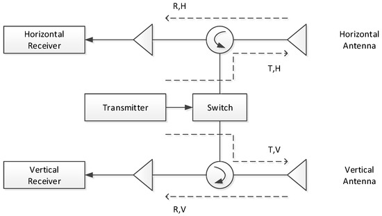
Figure 1.
The 2 × 2 R and T matrix system model architecture for radar polarimeters.
To this architecture for radar polarimeters, a measured scattering matrix M is related to an actual target scattering matrix S; where A represents the radar system gains and losses (in amplitude) and is any phase shift due to the round-trip delay between target and radar and any losses in the system. The receive and transmit matrices R and T describe the polarization characteristics of the radar system and signal transmission processes, including radar transmitter, transmit antenna, receive antenna, receiver, gain controller, ionosphere, and the like. The subscripts 1 and 2 correspond to H and V polarizations, with representing , the level of V contamination (subscript 2) on H transmit (subscript 1). Ideally, R and T should be identity matrices. The matrix N represents the additive noise voltage present in each radar channel.
After [35,37], the standard 2 × 2 R and T model (1) for a radar polarimeter has been widely used, sometimes for the convenience of application to make a simple distortion matrix [3,14,38]. Based on this and for the convenience of narration, we call this 2 × 2 R and T model (1) the classic system model for radar polarimeters, which is distinguished from the other system model for radar polarimeters [3].
Considering the ideal case, the additive noise is small, and the matrix N can be ignored, then the classic system model is simplified as:
For a meaningful quad-polarimetric radar system, the receive and transmit matrices R and T are all invertible. The estimated value of the distortion matrix R and T can be obtained through calibration experiments, then by (3), the estimation of the scattering matrix S can be obtained by polarization correction of the measured matrix M [2].
where the symbol ∧ above the parameter indicates an estimate of the corresponding parameter below it.
2.2. Improved System Model of GaoFen-3
The quad-polarimetric strip modes of GF-3 work in the time-division (TD) operation architecture [41]. The SAR system transmits horizontal (H) or vertical (V) polarization pulses in alternate pulse repeat frequency (PRF), whereas it receives backscattering signals in both H and V polarizations. Furthermore, inverse modulation slopes are employed in chirp signal transmitting of H and V polarization. As shown in Figure 2, the H polarization transmitting signal is modulated in the positive slope, and correspondingly, the V polarization is modulated in the negative slope. The inverse slopes in signal modulation can effectively suppress the cross-pol ambiguity generated by strong back-scattering ground objects [41].
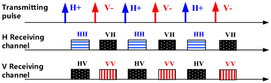
Figure 2.
GF-3 time-division operation architecture with inverse modulation slopes.
Since co-pol returns from natural terrain are generally 6–10 dB higher than cross-pol returns, this type of ambiguity is often 6–10 dB higher than is the case for a single-pol system [42]. To make better use of the dynamic range of the receivers and adapt to the difference between the scattering characteristics of the cross-pol and co-pol, there exists an MGC device in the H and V channels respectively of the GF-3, which would dynamically adjust the attenuation value according to the polarization type of the received signals. In general, the attenuation value of the co-pol is 10 dB larger than that of the cross-pol.
For this kind of working mechanism, each channel presents different amplitude and phase characteristics when receiving different types of polarimetric signals. If the error of the MGC device with different gain attenuation values is different, that is the MGC device is non-linear, the amplitude and phase characteristics of the receive channel would still be inconsistent even if the nominal gain attenuation value is corrected during data processing. Then, the system architecture of GF-3 is shown in Figure 3, which is significantly different from the architecture shown in Figure 1 that is suitable for the description by the classic polarimetric system model (1).
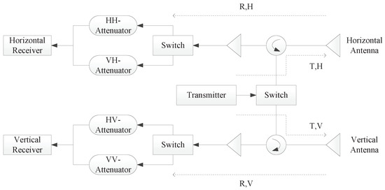
Figure 3.
System model architecture for GF-3.
Freeman has studied this issue earlier and proposed a general polarimetric system model [3], which is:
The parameter is a measure of the product of the gain error terms in the co-pol channels versus the cross-pol; i.e.,
According to the symmetry of the polarimetric system, the equation above would still hold if each element of the other co-pol channel is multiplied by or each element of any cross-pol channel is divided by , which could be inferred from the derivation of Freeman’s new model [3].
This general polarimetric system model contains a 4 × 4 polarimetric distortion matrix, and many elements of the distortion matrix are the product of two or three quantities, which cannot reflect the imbalance and cross-talk of the polarimetric system channels intuitively and will limit the use of the model.
When is equal to one, the classic system model and the general system model could be replaced with each other, though different in expression. Through appropriate mathematical transformation, the parameter could be removed from the distortion matrix , e.g., divide of the measure vector , the elements in the fourth row of the 4 × 4 distortion matrix , and the error vector by the factor, then the factor in the 4 × 4 distortion matrix is removed. Ignoring the additive noise, the model above could be written as:
After the correction of the elements of one channel of the measured matrix with the factor, the general polarimetric system can be described by a 2 × 2 matrix polarimetric model. The correction through the factor can be performed on any channel, that is dividing any element of the co-pol channels by or multiplying any element of the cross-pol channels by . Without loss of generality, we adopt the following form:
This is a general polarimetric system model, which has a 2 × 2 matrix form. Each parameter in the model has a clear and intuitive physical meaning, which we will describe in Appendix B. In Appendix A, we further deduce the applicable conditions of the classic polarimetric system model and point out that the parameter is the ratio of the system transfer functions of the co-pol channel and the cross-pol channel and is also a new imbalance factor. This corrected measured matrix is called a co-pol versus cross-pol balanced measured matrix of the radar polarimeter, referred to as a balanced measured matrix for short.
For the GF-3 satellite, as a result of the dynamic change of the MGC gain for each channel when receiving different types of polarimetric returns, the nonlinearity of the MGC device is manifested. Even if the MGC nominal gain is corrected, there still exists some amplitude and phase errors such that the system transfer functions of the four polarimetric channels become independent, causing the new imbalance factor not to be equal to one. Thus, the improved general polarimetric system model (7) is required to accurately describe the GF-3 polarimetric system.
Like Freeman’s model (4), the improved model can be applied to many practical polarimetric systems, and many polarimetric calibration methods based on the classic system model could be applicable after the correction of the measured matrix through the factor.
2.3. New Imbalance Factor Calibration Theory
For a radar polarimeter, suppose there is a point target P; the scattering matrix is , and a, b, c are not equal to zero, i.e.,
According to the improved system model (7), we have:
AS a, b, c are not equal to zero, matrices and are invertible, and is not equal to zero, then, normally, all four elements of the balanced measured matrix are not zero. By the nature of the right side of (9), that is, , then the new imbalance factor can be solved:
In practice, in order to avoid the influence of additive noise, the signal-to-noise ratio and signal-to-clutter ratio of the point target P in each polarimetric channel should be as high as possible. In the case of general measurement, the requirement can reach 30 dB.
Considering the scattering characteristics of the target, the commonly-used point target scattering matrix for estimating the new imbalance factor is: , , , , and so on.
The scattering matrix of the PARC is , which has the form of , where is defined on the normal plane of the radar sight and is the polarimetric orientation angle of the calibrator with respect to the local horizontal. When is chosen to be , , , or , the four elements of the scatter matrix are one or −1, and the calibrator is adapted to measure this new imbalance factor. In particular, as long as the signal-to-noise ratio and signal-to-clutter ratio of each channel meet the measurement requirements, need not be set very accurately, and the measurement of the new imbalance factor does not change. Therefore, the use of PARC to measure the new imbalance factor has a very high robustness.
2.4. Calibration Method Based on the Improved System Model
Based on the improved model, we improve Freeman’s polarimetric calibration method that uses a combination of three polarimetric active radar calibrators with scattering matrices [2]:
The quad-polarimetric measured matrices from these calibrators are:
The corresponding balanced measurement matrices corrected by the new imbalance factor are:
According to the improved general fully-polarimetric radar system model (7), we have:
Inherent in (14) is that the factor and the distortion matrices and do not change during the measurement of these three calibrators. The complex factors in front of the matrix product can, however, be different.
1 The new imbalance factor estimation algorithm
According to (10), the polarimetric active radar calibrator whose scattering matrix is is used to estimate the new imbalance factor; we have:
2 The distortion matrices and estimation algorithm
The solution to the distortion matrices is based on the Freeman algorithm [2], except that instead of calculating directly from the measured matrix, it is calculated from the balanced measured matrix; or we first correct the corresponding channel image with the new imbalance factor obtained from the above measurement and then solve the distortion matrices.
The distortion matrices and can be expressed in terms of the 12 measured quantities and the new imbalance factor as follows:
(1) Expressing in terms of and in terms of .
where:
or:
and:
where:
or:
(2) Expressing in terms of and in terms of .
where:
or:
and:
where:
or:
In the absence of noise, the two expressions for each should be equal.
3 Improved polarimetric correction algorithm of polarimetric radar image data
The inversion to estimate from its measured matrix is divided into two steps:
First, using the factor of (15) to correct the measured matrix for the co-pol versus cross-pol imbalance (note that the corrected polarimetric channel should be consistent with that when measured), obtain a balanced measured matrix .
Then, from the distortion matrices and and the balanced measured matrix , the estimation of the target scattering matrix is obtained according to the following.
or:
where the preceding complex term as a whole can be estimated by the following.
3. The GF-3 Calibration Experiment at Erdos Grassland
The Erdos grassland in Inner Mongolia is an ideal background against which to place calibration devices. The grassland is flat and behaves like a specular surface at C-bands of the spaceborne-SAR system, exhibiting a low that is usually less than −9 dB across this frequency/polarizations.
The GF-3 satellite successfully carried out four polarimetric calibration experiments in Erdos on 8 September 2016, 19 September 2016, 11 July 2017, and 16 July 2017. These experiments involved 5 PARCs, 9 triangular corner reflectors, 3 dihedral corner reflectors, and 1 dihedral corner reflector. Due to conditions such as site, equipment status, preparation time, and manpower, not every device participated in each test. Among the experiments, the first used 5 PARCs, 3 trihedral corner reflectors (TCRs), and 3 dihedral corner reflectors (DCRs); the second used 3 PARCs, 2 TCRs, 1 DCR, and 1 DCR; the third used 3 PARCs and 7 TCRs; the forth used 3 PARCs and 9 TCRs. Figure 4 shows one of the PARCs deployed at the grassland for the GF-3 experiment, and Figure 5 shows one of the TCRs deployed.
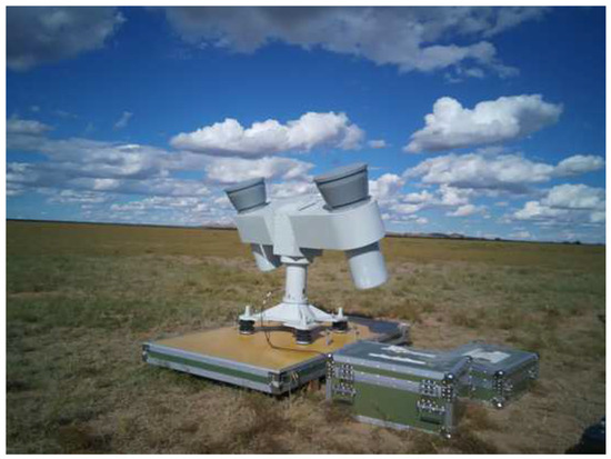
Figure 4.
One of the polarimetric active radar calibrators (PARCs) deployed at the grassland for the GF-3 experiment.
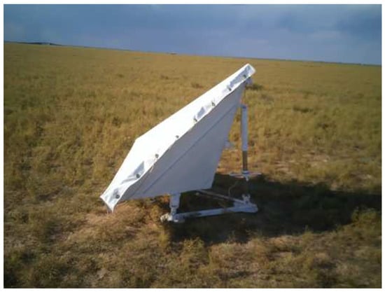
Figure 5.
One of the trihedral corner reflectors (TCRs) deployed at the grassland for the GF-3 experiment.
The polarimetric active radar calibrators PARC-1, PARC-2, and PARC-3 were for the polarimetric distortion matrices and the new imbalance factor measurement. In order to eliminate changes in the radar system parameters along the range direction, the three calibrators were located in relatively close positions. The polarimetric scattering matrices were:
For other calibration devices for polarization accuracy testing, the polarimetric active radar calibrators PARC-4 and PARC-5, the scattering matrices were:
The scattering matrices of the trihedral corner reflectors, dihedral corner reflectors, and dihedral corner reflector were:
The imaging parameters of the GF-3 satellite in the four experiments are shown in Table 1.

Table 1.
The working parameters of GaoFen-3 (GF-3) for the calibration tests. MGC, manual gain control.
4. Data Processing, Results, and Discussion
The original image data required for the external calibration test analysis were corrected according to the method of Sha Jiang in [43] by internal calibration data. According to Sha Jiang’s analysis in [43], the Faraday rotation angle of the GF-3 satellite is generally no more than , and its influence can be ignored. At the same time, in order to focus on the main issues, we do not discuss the Faraday rotation angle here.
4.1. The Data Processing Results of the Two Algorithms
The extracted polarimetric distortion parameters, i.e., , R and T, are as shown in Table 2 using the improved calibration algorithm. Then, the images were corrected using the extracted polarimetric distortion parameters, and the polarization characteristic matrices of main calibration devices were extracted as shown in Table 3 (due to the length of the occupation, the third and fourth tests only listed the data of three TCRs, and the data of other TCRs were similar to the listed data). The results of the four test treatments showed that was not equal to or close to one for the GF-3 satellite. If the classic polarimetric system model were used to describe the polarization characteristics of the GF-3 satellite and for the polarimetric calibration, significant errors would result. Table 4 shows the polarimetric distortion matrices, which were extracted by Freeman’s algorithm used in [2] based on the classic model. Table 5, which corresponds to Table 3, shows the polarization characteristics matrices of main calibration equipments after correction by the polarimetric distortion matrices in Table 4.
Table 2.
The extracted polarimetric distortion parameters by the improved algorithm of this paper.
Table 3.
The correction results by the polarimetric parameters from the improved algorithm of this paper.
Table 4.
The extracted polarimetric distortion matrices of Freeman’s algorithm in [2].
Table 5.
The correction results by the polarimetric distortion matrices from Freeman’s algorithm.
4.2. GF-3 Radar Polarization Performance: Further Analysis
In these experiments, the active radar calibrators RCS value was set to 60 dBsm, to meet the GF-3 polarization isolation measurement requirements. The trihedral and dihedral corner reflectors with RCS 35 dBsm were not good devices for measuring polarization isolation, as the signal clutter ratio was not high. Therefore, we used the test data of PARC-4 and PARC-5 on 8 September 2016 to measure the radar polarization isolation. According to the measurement results in Table 3, the minimum polarization isolation of the system can reach −38.2 dB.
Because of the good stability of the trihedral and dihedral corner reflector, it can be used to assess the polarimetric radar channel amplitude and phase imbalance. However, due to the channel inconsistency, the active radar calibrator will introduce a large error in the assessment of channel amplitude and phase imbalance, which is not suitable as a device for evaluating the amplitude and phase imbalance. Here, the trihedral and dihedral corner reflector were used as a method to evaluate the amplitude and phase imbalance of the polarimetric system. According to the measurement results in Table 3, for co-pol channels, the imbalance of amplitude can reach 0.7 dB, and the phase imbalance was no greater than . For cross-pol channels, the imbalance of amplitude can reach 0.3 dB, and the phase imbalance was no greater than .
5. Conclusions
In this paper, we introduce a new imbalance parameter into the classic system model and propose an improved system model for GF-3. This improved model maintains a 2 × 2 matrix form and contains seven polarimetric parameters, and all parameters have clear physical meanings. Like Freeman’s model (4) [3], the improved model has universal applicability and could be applied to various practical polarimetric radars. Based on this, polarimetric radars can be divided into two basic types, balanced and unbalanced for the co-pol versus cross-pol channels. For balanced polarimetric radars, the new imbalance parameter is equal to one, and the improved model is equivalent to the classic system model. For unbalanced polarimetric radars, the new imbalance parameter is not equal to one and must be corrected by this new imbalance parameter, and then, it can be described using the classic system model, which is the essence of the improved model. Then, we propose the calibration theory of the new imbalance parameter, point out that the calibration method of the new imbalance parameter using PARC is not affected by the calibrator’s orientation angle error and has very good robustness, and improve Freeman’s polarimetric calibration algorithm based on three PARCs. From the analysis of published literature data, we find that some well-known polarimetric radar systems are also unbalanced for the co-pol versus cross-pol channels. Just like GF-3, such systems are practical and universal, and these systems can be more accurately described with the improved model.
In summary, our GF-3 calibration data processing results indicate that the improved system model for radar polarimeters and the improved calibration algorithm using adjacent PARCs gave good results, and these verify the effectiveness of the theory of the paper. This paper has carried out a rigorous theory deduction, and the improved model and the algorithm have quite general adaptability and can be applied to other satellite and airborne fully-polarimetric radar systems’ calibration and the data processing. Based on the improved model, other polarimetric calibration methods can also be improved to make them suitable for general polarimetric radar systems.
Author Contributions
Methodology, W.L.; software, W.L., Z.J.; validation, X.Q., Z.D.; formal analysis W.L., X.Q. and J.H.; investigation, Z.J., Z.D.; resources, B.L., Q.Z. and A.W.; data curation, Z.J., Z.D.; writing—original draft preparation, W.L., F.Z.; writing—review and editing, W.L., Z.D.; visualization, W.L.; supervision, J.H., X.Q.; project administration, B.L., Q.Z. All authors read and approved the final version of the manuscript.
Funding
This work was supported in part by the project of the GaoFen-3 SAR calibration processing system under Grant No. Y5H2980402.
Acknowledgments
The authors would like to thank the GF-3 SAR Satellite Group for the satellite and ground system development work, the staff of the China Center for Resources Satellite Data and Application for their help, and the members of the calibration team for their efforts in deploying equipment at the Erdos calibration site in Inner Mongolia, China. Thanks to Guangjing Cao for helping to typeset the document.
Conflicts of Interest
The authors declare no conflict of interest. The funders had no role in the design of the study; in the collection, analyses, or interpretation of data; in the writing of the manuscript, or in the decision to publish the results.
Appendix A. Adaptation Conditions of Classic Model
From (2) and (3), we can get (A1), i.e., the rank of the actual target scattering matrix S is equal to the rank of the measurement scattering matrix M, and both matrices are either invertible or irreversible.
For the radar polarimeter systems with an architecture similar to the one illustrated in Figure 1, for the cross-talk distortion that can be separated from the channel imbalance distortion [10], the system transfer function model can be described by Figure A1. From this perspective of the system transfer function, for the radar polarimeters whose system models are (1) and (2), considering each polarimetric channel individually and ignoring the additive noise ideally, the following Equation (A2) holds [16].
where is the measured scattering value of the target by the channel of a radar polarimeter, represents the system transfer function of the channel, which is the amplitude and phase imposed by the radar and the signal transmission processes on the backscatter measurement, is the pure (or true) scattering characteristic of the target from polarization p on transmit and q on receive, and is the scattering characteristic of the target observed by the channel, which is similar to a single-polarimetric system with polarization p on transmit and q on receive. Due to the mutual coupling between the channels, the observed target scattering characteristic by the channel is a function of the quad-polarimetric scattering characteristics of the target, i.e., . As a whole, the observed target scattering matrix in this polarimetric radar state is the primary transformation of the target true scattering matrix , that is there exists invertible matrix , , so that:

Figure A1.
System transfer function model for radar polarimeters.
According to the six polarimetric parameters’ form of the classic system model [2,10], and can be obtained, where non-zero non-diagonal elements indicate that signal coupling will occur and cross-talk will be introduced. In general, these non-diagonal elements are closer to zero, and matrix and are invertible, then the ranks of matrices and are equal:
Substitute (A2) into the measured scattering matrix , and get (A5), which is another form of .
Substitute (A5) into (2), and get (A6), which is another form of the classic system model (2).
Here, we redefine the parameter in the following (A7) as the ratio of the system transfer functions of co-pol versus cross-pol channels, which is a complex, and describes the relationship between the system transfer functions of the four channels.
According to (A1), (A4), and (A6), the parameter is mathematically deduced to be one, that is (A8) holds. The actual derivation is included in Appendix C.
After mathematical deduction in Appendix D, for (A6), only when (A8) is established, that is the parameter is equal to one, can (A1) be established.
In summary, for (2) and (A5), that is for (A6), (A1) and (A8) are equivalent.
Therefore, the new parameter equal to one is an essential feature for the radar polarimeters whose system models are (1) and (2). In other words, the classic system model (1), (2) is valid only when the new parameter is equal to one.
indicates that the system transfer functions of the four polarimetric channels are related and not independent of each other, that is only three of the four system transfer functions are independent, so that two parameters can be used to describe the relative relationship between the four channels. These two parameters are usually the channel imbalance terms for receivers and transmitters [2], which are usually represented by and .
For (A5), only when the parameter is equal to one can (A6) be established; the invertible matrices and exist, and thus, we can obtain the scattering matrix from the measured matrix by Equation (3). This measured matrix when is called a co-pol versus cross-pol balanced measured matrix of the radar polarimeter, referred to as a balanced measured matrix for short.
When , the new parameter describes the amplitude and phase imbalance of the co-pol versus cross-pol channels, which can be called the amplitude and phase imbalance factor of the co-pol versus cross-pol channels in a fully-polarimetric system, and this is the third and new imbalance term, which is independent of the channel imbalance terms for receivers and transmitters, i.e., and .
Appendix B. Another Derivation Process of the General Polarimetric System Model
For a fully-polarimetric radar like Figure 1, due to the imperfect time stability and the linear inaccuracy in the dynamic range, as well as the constant changes of environmental factors, the random signal transmission in the atmosphere, etc., each channel system transfer function will introduce error, and this error is a multiplicative error; the quad-channel system transfer function changes cannot be synchronized, so that the factor is not equal to one, that is the system degenerated into the quad-channel system transfer function independent fully-polarimetric radar, the architecture shown in Figure 3. The architecture of this degenerated polarimetric radar is essentially the same as that of the fully-polarimetric radar mentioned in Freeman’s article [2], where the system transfer functions of the quad-polarimetric channels are independent of one another, and is a practical, more general polarimetric system architecture.
For these radar polarimeters, the factor is not equal to one, and based on Appendix A, the classic system model (1), (2) is invalid for them. For (A5), matrix is not a balanced measured matrix. We use the definition of the factor in (A7) to correct an element of the matrix (The correction of the factor is a relativity correction that can correct for any one element of the measured matrix , diagonal element correction divided by , non-diagonal element correction multiplied by . Here, the element in the lower left corner is corrected.) and get a balanced measured matrix as follows (A9).
where , , , are the four elements of the measured matrix .
For the balanced measured matrix , it can be seen that the new quad-channel system transfer functions, which are , , , and , are related, and the corrected new factor is equal to one. Therefore, the ranks of matrix and are equal, and there are the invertible matrices and , so that (A10) (or (7); the two are the same) holds. This is an improved system model and solves the problem that the classic system model (1), (2) fails to do when the factor is not equal to one.
In (2), the distortion matrices and are respectively normalized to obtain another form of classic system model with six polarimetric parameters [3,35]. Combining (A10), another form of the improved model can be obtained, that is a system model with seven polarimetric parameters, i.e.,
where , and are channel imbalance terms for receivers and transmitters, respectively, and the ’s are cross-talk terms representing the cross-pol isolation of the system. (A11) describes the process of stepwise distortion of the target polarimetric characteristics.
Since is a complex, the correction of the new imbalance factor is a uniform correction of the relative amplitude and phase between the quad-polarimetric channels, which is different from the radiation correction for each of the quad-polarimetric channels, and therefore, radiation correction cannot replace this correction. Since the classic system model (1), (2) is invalid for the general radar polarimeters with the system architecture of Figure 3, the corresponding polarimetric distortion matrices and do not exist, so the correction of the factor is also different from the polarimetric distortion matrix correction. This correction of the new imbalance factor belongs to the category of polarization correction.
A fully-polarimetric radar with the factor equal to or close to one means that the quad-channel system transfer functions are related and can be called a balanced fully-polarimetric radar for co-pol versus cross-pol channels. Conversely, the more the factor deviates from one, the more the system transfer function of the four channels of the fully-polarimetric radar is uncorrelated or independent, and it can be called an unbalanced fully-polarimetric radar for the co-pol versus cross-pol channels; and such a radar must be corrected by the factor , then it can be accurately described. Therefore, the factor is an important parameter to describe the performance of a fully-polarimetric radar.
The improved general system model, with a standard 2 × 2 matrix form, which is different from Freeman’s general model using a Kronecker-delta matrix format [2], is as easy to use as the classic system model, and every parameter has a clear physical meaning. In addition, the improved general model unifies the polarimetric system model in terms of expression. It can be seen that the classic model is just a special case, representing a linear system as a special case.
Appendix C. Proof: (A1) Holds, Then (A8) Holds
From (A1) and (A4), we get:
Based on (A4), assuming there is a class of targets whose scattering matrix has the following properties:
and:
for example, the target to meet the above conditions (A13), (A14). From (A12), (A13), then:
and we get:
From (A14), (A16), (A17), we get:
for the system transfer function is not zero, and we get:
that is, (A8) holds.
Appendix D. Proof: (A8) Holds, Then (A1) Holds
According to the scattering matrix rank, the following proof is divided into three cases.
Case 1:
Then:
and from (A5), we get:
then:
Case 2:
Then:
and , , , and ; at least one is not zero, so the assumption is:
From (A7), (A8), we get:
Substitute (A25) into (A23), and we get:
From (A24), (A25), we get:
From (A26), (A27), we get:
Case 3:
Then:
From (A7), (A8), we get:
Substitute (A30) into (A29), and we get:
then:
In summary, from (A22), (A28), (A32), we get:
that is, (A1) holds.
References
- Sheen, D.R.; Freeman, A.J.; Kasischke, E.S. Phase calibration of polarimetric radar images. IEEE Trans. Geosci. Remote Sens. 1989, 27, 719–731. [Google Scholar] [CrossRef]
- Freeman, Y.S.A.; Werner, C. Polarimetric radar calibration experiment using active radar calibrators. IEEE Trans. Geosci. Remote Sens. 1990, 28, 224–240. [Google Scholar] [CrossRef]
- Freeman, A. A new system model for radar polarimeters. IEEE Trans. Geosci. Remote Sens. 1991, 29, 761–767. [Google Scholar] [CrossRef]
- Quegan, S. A unified algorithm for phase and cross-talk calibration of polarimetric data-theory and observations. IEEE Trans. Geosci. Remote Sens. 1994, 32, 89–99. [Google Scholar] [CrossRef]
- Zebker, H.A.; Zyl, J.J.; Durden, S.L.; Norikane, L. Calibrated imaging radar polarimetry: Technique, examples, and applications. IEEE Trans. Geosci. Remote Sens. 1991, 29, 942–961. [Google Scholar] [CrossRef]
- Zebker, H.A.; Zyl, J.J. Imaging radar polarimetry: A review. Proc. IEEE 1991, 79, 1583–1606. [Google Scholar] [CrossRef]
- Satake, M.; Kobayshi, T.; Manabe, T.; Masuko, H. Polarimetric calibration of x-band airborne synthetic aperture radar using corner reflectors and an active radar calibrator. In Proceedings of the 1998 IEEE International Geoscience and Remote Sensing, Symposium Proceedings, Seattle, WA, USA, 6–10 July 1998; Volume 2, pp. 660–662. [Google Scholar]
- Christensen, E.L.; Skou, N.; Dall, J.; Woelders, K.W.; Jorgensen, J.H.; Granholm, J.; Madsen, S.N. Emisar: An absolutely calibrated polarimetric l-and c-band sar. IEEE Trans. Geosci. Remote Sens. 1998, 36, 1852–1865. [Google Scholar] [CrossRef]
- Ainsworth, T.L.; Ferro-Famil, L.; Lee, J.S. Orientation angle preserving a posteriori polarimetric sar calibration. IEEE Trans. Geosci. Remote Sens. 2006, 44, 994–1003. [Google Scholar] [CrossRef]
- Shimada, M.; Kawano, N.; Watanabe, M.; Motooka, T.; Ohki, M. Calibration and validation of the pi-sar-l2. In Proceedings of the 2013 Asia-Pacific Conference on Synthetic Aperture Radar (APSAR), Tsukuba, Japan, 23–27 September 2014; Volume 478, pp. 194–197. [Google Scholar]
- Satake, M.; Kobayashi, T.; Uemoto, J.; Umehara, T.; Kojima, S. Polarimetric calibration of pi-sar2. In Proceedings of the 2013 Asia-Pacific Conference on Synthetic Aperture Radar (APSAR), Tsukuba, Japan, 23–27 September 2013; pp. 79–80. [Google Scholar]
- Ming, F.; Hong, J.; Zhang, L. Improved calibration method of the airborne polarimetric sar. In Proceedings of the 2011 3rd International Asia-Pacific Conference on Synthetic Aperture Radar (APSAR), Seoul, Korea, 26–30 September 2011; pp. 1–3. [Google Scholar]
- Williams, M.L.; Stacy, N.; Badger, D.; Preiss, M.; Preiss, A. Calibration and Performance Validation of the Ingara, High Resolution, Fully Polarimetric, x-Band Sar. In Proceedings of the CEOS Workshop on Polarimetric SAR, Ulm, Germany, 27–28 May 2004. [Google Scholar]
- Fujita, Y.F.M.; Masuda, T.; Satake, M. Polarimetric calibration of the sir-c c-band channel using active radar calibrators and polarization selective dihedrals. IEEE Trans. Geosci. Remote Sens. 1998, 36, 1872–1878. [Google Scholar] [CrossRef]
- Freeman, A. Sir-c calibration results. Math. Comput. Model. 2001, 33, 695–706. [Google Scholar]
- Freeman, A.; Alves, M.; Chapman, B.; Cruz, J. Sir-c data quality and calibration results. IEEE Trans. Geosci. Remote Sens. 1995, 33, 848–857. [Google Scholar] [CrossRef]
- Masaharu Fujita, Y.F.; Satake, M. Sir-c polarimetric calibration by using polarization selective dihedrals and a polarimetric active radar calibrator. Geosci. Remote Sens. 1997, 4, 1941–1943. [Google Scholar]
- Kimura, H. Calibration of polarimetric PALSAR imagery affected by faraday rotation using polarization orientation. IEEE Trans. Geosci. Remote Sens. 2009, 47, 3943–3950. [Google Scholar] [CrossRef]
- Sandberg, G.; Eriksson, L.E.B.; Ulander, L.M.H. Measurements of faraday rotation using polarimetric palsar images. IEEE Geosci. Remote Sens. Lett. 2009, 6, 142–146. [Google Scholar] [CrossRef]
- Touzi, R.; Shimada, M. Polarimetric PALSAR Calibration. IEEE Trans. Geosci. Remote Sens. 2009, 47, 3951–3959. [Google Scholar] [CrossRef]
- Shimada, M. Model-based polarimetric sar calibration method using forest and surface-scattering targets. IEEE Trans. Geosci. Remote Sens. 2011, 49, 1712–1733. [Google Scholar] [CrossRef]
- Meyer, F.J.; Nicoll, J.B. Prediction, detection, and correction of faraday rotation in full-polarimetric l-band sar data. IEEE Trans. Geosci. Remote Sens. 2008, 46, 3076–3086. [Google Scholar] [CrossRef]
- Touzi, R.; Hawkins, R.K.; Cote, S. High-Precision Assessment and Calibration of Polarimetric RADARSAT-2 SAR Using Transponder Measurements. IEEE Trans. Geosci. Remote Sens. 2013, 51, 487–503. [Google Scholar] [CrossRef]
- Iannini, G.L.; Tebaldini, S. Long term relative polarimetric calibration by natural targets. In Proceedings of the 2013 IEEE International Geoscience and Remote Sensing Symposium, Melbourne, VIC, Australia, 21–26 July 2014. [Google Scholar]
- Caves, R. Radarsat-2 polarimetric calibration performance over five years of operation. In Proceedings of the 10th European Conference on Synthetic Aperture Radar, Berlin, Germany, 3–5 June 2014; pp. 1–4. [Google Scholar]
- Moriyama, T. Polarimetric calibration of palsar2. In Proceedings of the 2015 IEEE International Geoscience and Remote Sensing Symposium, Milan, Italy, 26–31 July 2015; Volume 9, pp. 1284–1287. [Google Scholar]
- Touzi, R.; Shimada, M. Calibration and validation of polarimetric alos2. In Proceedings of the 2015 IEEE International Geoscience and Remote Sensing Symposium, Milan, Italy, 26–31 July 2015; pp. 4113–4116. [Google Scholar]
- Zhang, Q. System design and key technologies of the gf-3 satellite. Acta Geod. Cartogr. Sin. 2017. [Google Scholar] [CrossRef]
- Liu, J.; Qiu, X.; Hong, W. Automated ortho-rectified sar image of gf-3 satellite using reverse-range-doppler method. J. Geophys. Res. Solid Earth 2016, 12, 4445–4448. [Google Scholar]
- Jiang, S.; Qiu, X.; Han, B.; Hu, W. A quality assessment method based on common distributed targets for gf-3 polarimetric sar data. Sensors 2018, 18, 807. [Google Scholar] [CrossRef]
- Sarabandi, K.; Pierce, L.E.; Ulaby, F.T. Calibration of a polarimetric imaging SAR. IEEE Trans. Geosci. Remote Sens. 1992, 30, 540–549. [Google Scholar] [CrossRef]
- Sarabandi, K. Calibration of a polarimetric synthetic aperture radar using a known distributed target. IEEE Trans. Geosci. Remote Sens. 1994, 32, 575–582. [Google Scholar] [CrossRef]
- Sarabandi, K.; Pierce, L.E. Cross-calibration experiment of JPL AIRSAR and truck-mounted polarimetric scatterometer. IEEE Trans. Geosci. Remote Sens. 1994, 32, 975–985. [Google Scholar] [CrossRef]
- Klein, J.D. Calibration of complex polarimetric sar imagery using backscatter correlations. IEEE Trans. Aerosp. Electron. Syst. 1992, 28, 183–194. [Google Scholar] [CrossRef]
- Van Zyl, J.J. Calibration of polarimetric radar images using only image parameters and trihedral corner reflector responses. IEEE Trans. Geosci. Remote Sens. 1990, 28, 337–348. [Google Scholar] [CrossRef]
- Freeman, A.; Zyl, J.J.V.; Klein, J.D. Calibration of Stokes and scattering matrix format polarimetric SAR data. IEEE Trans. Geosci. Remote Sens. 1992, 30, 531–539. [Google Scholar] [CrossRef]
- Zebker, H.A.; Zyl, J.J.; Held, D.N. Imaging radar polarimetry from wave synthesis. J. Geophys. Res. Solid Earth 1987, 92, 683–701. [Google Scholar] [CrossRef]
- Freeman, A. Calibration of linearly polarized polarimetric sar data subject to faraday rotation. IEEE Trans. Geosci. Remote Sens. 2004, 42, 1617–1624. [Google Scholar] [CrossRef]
- Li, L.; Zhu, Y.; Hong, J. Design and Implementation of a Novel Polarimetric Active Radar Calibrator for Gaofen-3 SAR. Sensors 2018, 18, 2620. [Google Scholar] [CrossRef]
- Whitt, M.W.; Ulaby, F.T.; Polatin, P. A general polarimetric radar calibration technique. IEEE Trans. Anttenas Propag. 1991, 39, 62–67. [Google Scholar] [CrossRef]
- Sun, J.; Yu, W.; Deng, Y. The SAR Payload Design and Performance for the GF-3 Mission. Sensors 2017, 17, 2419. [Google Scholar] [CrossRef] [PubMed]
- Freeman, A. On the design of spaceborne polarimetric SARs. In Proceedings of the IEEE Radar Conference, Pasadena, CA, USA, 4–8 May 2009; pp. 1–4. [Google Scholar]
- Jiang, S.; Qiu, X.; Han, B.; Sun, J.; Ding, C. Error Source Analysis and Correction of GF-3 Polarimetric Data. Remote Sens. 2018, 10, 1685. [Google Scholar] [CrossRef]
© 2019 by the authors. Licensee MDPI, Basel, Switzerland. This article is an open access article distributed under the terms and conditions of the Creative Commons Attribution (CC BY) license (http://creativecommons.org/licenses/by/4.0/).