Parameterized Nonlinear Least Squares for Unsupervised Nonlinear Spectral Unmixing

Abstract

This paper presents a new parameterized nonlinear least squares (PNLS) algorithm for unsupervised nonlinear spectral unmixing (UNSU). The PNLS-based algorithms transform the original optimization problem with respect to the endmembers, abundances, and nonlinearity coefficients estimation into separate alternate parameterized nonlinear least squares problems. Owing to the Sigmoid parameterization, the PNLS-based algorithms are able to thoroughly relax the additional nonnegative constraint and the nonnegative constraint in the original optimization problems, which facilitates finding a solution to the optimization problems . Subsequently, we propose to solve the PNLS problems based on the Gauss–Newton method. Compared to the existing nonnegative matrix factorization (NMF)-based algorithms for UNSU, the well-designed PNLS-based algorithms have faster convergence speed and better unmixing accuracy. To verify the performance of the proposed algorithms, the PNLS-based algorithms and other state-of-the-art algorithms are applied to synthetic data generated by the Fan model and the generalized bilinear model (GBM), as well as real hyperspectral data. The results demonstrate the superiority of the PNLS-based algorithms.

1. Introduction

Due to the spatial resolution limitation of hyperspectral remote sensors as well as the diversity of surface features, mixed pixels are a common occurrence in hyperspectral images. Spectral unmixing is an essential technique for analyzing mixed pixels which extracts a collection of spectral signatures or endmembers and their corresponding fractions (abundances) contained in the mixed pixels. A large number of unmixing algorithms have been proposed based on the linear mixture model (LMM), which assumes that the spectrum of the mixed pixels is a linear combination of several endmembers. The linear unmixing process involves extracting the endmembers [1] and estimating their abundances [2] or obtaining endmembers and abundances simultaneously [3,4,5].

Nevertheless, the LMM cannot necessarily reflect the true composition of real-world scenarios such as planetary remote sensing, intimate mineral mixtures, vegetation canopies, or urban scenes [6]. Therefore, kernels are popularly adopted to introduce nonlinearities in unmixing [7,8,9], which is independent of specific mixing models. However, the kernel-based methods largely depend on the choice of the kernel functions and parameters [6]. On the other hand, physical models based on the the nature of environment have been proposed to overcome the limitation of the LMM, including the Hapke model proposed in [10] and the bilinear mixture models (BMMs) [6]. In BMMs, the light probably undergoes secondary reflections or bilinear interactions before reaching the sensor. Different assumptions on the abundance constraints or bilinear parameters result in different expressions of the BMMs, such as the polynomial post-nonlinear model [11], the Nascimento model [12], the Fan model [13], and the generalized bilinear model (GBM) [14]. Several supervised nonlinear unmixing algorithms based on BMMs has been developed [14,15,16]. However, due to the lack of an endmember updating process, the unmixing performance of these supervised nonlinear unmixing algorithms is limited and greatly influenced by the accuracy of the endmember extraction methods [16], e.g., vertex component analysis (VCA) [1], pixel purity index (PPI) [17], simplex growing algorithm (SGA) [18] or N-FINDR algorithm [19]. To alleviate the limitations of supervised nonlinear unmixing, the unsupervised nonlinear spectral unmixing (UNSU) provides a viable option and some attempts have been made to estimate simultaneously the endmembers and abundances (or nonlinearity coefficients) for nonlinear mixing models. For example, the polynomial post-nonlinear mixing model (PPNMM) has been solved with an unsupervised method using a Hamiltonian Monte Carlo Algorithm [20] and has been shown to result in a better unmixing performance than the supervised method [15]. In [21], the authors provide an UNSU method for the Fan model using the NMF (Fan-NMF), which is proved to obtain better performance than the supervised or unsupervised LMM-based methods or the supervised GBM-based methods. In [22], we have also proposed an NMF-based UNSU method for the GBM (GBM-NMF).

In NMF-based methods, the physical constraints on the endmembers (nonnegativity) and abundances (nonnegativity and sum-to-one) are taken into consideration by means of a projected gradient (PG) update algorithm. The PG method is originally proposed by Lin [23] and provides a faster convergence than the multiplicative update rules designed by Lee and Seung [24]. However, NMF-based UNSU methods suffer from two problems. First, the simple projection step in the PG of setting negative values to zero or small positive values to impose non-negativity makes it difficult to provide a theoretical analysis of its convergence [25]. The projection step is likely to increase the objective function and may cause non-monotonic changes in the objective function, resulting in inaccurate factorization [26]. Second, only the first derivatives are used for updating in the NMF-based UNSU methods, which is inefficient for solving nonlinear mixing models since the endmembers to be estimated have strong interactions due to the existence of virtual endmembers, which are generated by the Hadamard product mathematically.

To further alleviate the problems of the NMF-based UNSU methods, in this study, we propose two well-designed UNSU methods based on parameterized nonlinear least squares (PNLS) for the widely used GBM and Fan model. In the proposed methods, the optimization problem for the UNSU is transformed into two (for Fan model) or three (for GBM) alternate linear/nonlinear least squares (LS/NLS) problems. To avoid the simple projection step which ensures nonnegativity, the unknown endmembers, abundances, and nonlinearity coefficients (only for the GBM) are parameterized by a Sigmoid function. In this way, the LS/NLS problems with additional constraints are transformed into PNLS problems free of constraints. The Gauss–Newton method is then utilized to alternately solve the unconstrained PNLS problems rather than the PG method used in the NMF-based UNSU methods. The proposed PNLS-based UNSU algorithms can obtain the endmembers, abundances, and nonlinearity coefficients (only for the GBM) simultaneously. The experimental results of synthetic and real data have verified that the proposed algorithms achieve better unmixing performance than the NMF-based UNSU algorithms for the GBM and the Fan model.

The remainder of this paper is organized as follows: Section 2 provides a brief review of the GBM and Fan model; Section 3 details the proposed PNLS-based UNSU algorithms; Section 4 presents and analyses a series of experiments using both synthetic and real hyperspectral data; Section 5 concludes this paper.

2. Bilinear Mixing Models

This section provides a brief introduction to the general form of two widely used bilinear models including the GBM and the Fan model.

2.1. GBM

The GBM is derived from the combination of an LMM and an additional nonlinear effect term, which emphasizes the second-order scattering effect. Let $\mathit{X}\in {\Re }^{L\times N}$ be any hyperspectral image with L bands and N pixels, then the nth pixel ${\mathit{x}}_n$ in $\mathit{X}$ can be represented using the GBM as follows [16]:

$${\mathit{x}}_n=\sum _{p=1}^P{\mathit{m}}_p{\mathit{A}}_{p,n}+\sum _{p=1}^{P-1}\sum _{q=p+1}^P{\mathit{B}}_{(p,q),n}{\mathit{m}}_p\odot {\mathit{m}}_q+\mathit{ffl},$$

(1)

with constraints

$$\sum _{p=1}^P{\mathit{A}}_{p,n}=1,{\mathit{A}}_{p,n}\ge 0,0\le {\mathit{B}}_{(p,q),n}\le {\mathit{A}}_{p,n}{\mathit{A}}_{q,n},{\mathit{m}}_p\ge 0,$$

(2)

where the first term on the right side of the Equation (1) indicates the linear mixing effect and the second term indicates the nonlinear mixing effect. ${\mathit{m}}_p$ denotes the pth endmember in the endmember matrix $\mathit{M}\in {\Re }^{L\times P}$ and ${\mathit{A}}_{p,n}$ denotes the corresponding abundance of ${\mathit{m}}_p$ in the pixel ${\mathit{x}}_n$. ⊙ denotes the Hadamard product between two vectors. ${\mathit{B}}_{(p,q),n}$ is the nonlinearity coefficient controlling the significance of the nonlinear effect. The subscript $(p,q)$ means that the item is derived from or associated with ${\mathit{A}}_{p,n}$ and ${\mathit{A}}_{q,n}$. $\mathit{ffl}$ represents the additional noise. It is noticed that apart from the nonnegative constraint, an upper bound constraint is also imposed on $\mathit{B}$. They are collectively called the boundary constraint hereinafter unless otherwise specified.

2.2. Fan Model

The Fan model can be regarded as a special case of the GBM where ${\mathit{B}}_{(p,q),n}={\mathit{A}}_{p,n}{\mathit{A}}_{q,n}$ instead of the constraint $0\le {\mathit{B}}_{(p,q),n}\le {\mathit{A}}_{p,n}{\mathit{A}}_{q,n}$, i.e., the Fan model has the following expression:

$${\mathit{x}}_n=\sum _{p=1}^P{\mathit{A}}_{p,n}{\mathit{m}}_p+\sum _{p=1}^{P-1}\sum _{q=p+1}^P{\mathit{A}}_{p,n}{\mathit{A}}_{q,n}{\mathit{m}}_p\odot {\mathit{m}}_q+\mathit{ffl}$$

(3)

with constraints:

$$\sum _{p=1}^P{\mathit{A}}_{p,n}=1,{\mathit{A}}_{p,n}\ge 0,{\mathit{m}}_q\ge 0.$$

(4)

3. Proposed PNLS

In this section, we present the proposed PNLS for the GBM and the Fan model. As the derivations of the PNLS for both models are quite similar, we only show the detailed derivation of the PNLS for the GBM and the PNLS for the Fan model will be given directly.

3.1. Definition of the Alternate LS/NLS Problems

Based on the GBM in (1), the UNSU problem can be defined as three alternate LS/NLS optimization problems for the local optimal solution of the endmembers, abundances, and nonlinearity coefficients.

3.1.1. Constrained NLS for Endmembers Estimation

To define the endmembers estimation as an NLS problem, the pixel-wise or column-wise form defined in Equation (1) should be transformed into the band-wise or row-wise form as follows:

$${\mathit{x}}_l={\mathit{m}}_l\mathit{A}+{\mathit{z}}_l\mathit{B}+\mathit{ffl}$$

(5)

with constraints:

$$\sum _{p=1}^P{\mathit{A}}_{p,n}=1,{\mathit{A}}_{p,n}\ge 0,0\le {\mathit{B}}_{(p,q),n}\le {\mathit{A}}_{p,n}{\mathit{A}}_{q,n},{\mathit{m}}_l\ge 0,$$

(6)

where ${\mathit{x}}_l,{\mathit{m}}_l,{\mathit{z}}_l$ are row vectors denote the lth row of $\mathit{X},\mathit{M},\mathit{Z}$ respectively and $\mathit{Z}=[{\mathit{m}}_1\odot {\mathit{m}}_2,{\mathit{m}}_1\odot {\mathit{m}}_3,\dots ,{\mathit{m}}_{P-1}\odot {\mathit{m}}_P]$ is the virtual endmember matrix. For the endmembers estimation, the abundances and nonlinearity coefficients are assumed to be fixed. Thus the constraints with respect to the abundances and nonlinearity coefficients can be neglected and the following constrained NLS problem is obtained:

$${\mathit{m}}_l=\underset{{\mathit{m}}_l}{\arg \min }{\parallel {\mathit{x}}_l-{\mathit{m}}_l\mathit{A}-{\mathit{z}}_l\mathit{B}\parallel }_2,\mathrm{s}.\mathrm{t}.{\mathit{m}}_l\ge 0.$$

(7)

3.1.2. Constrained LS for Abundances Estimation

The endmembers $\mathit{M}$, virtual endmembers $\mathit{Z}$, and nonlinearity coefficients $\mathit{B}$ are supposed to be fixed when updating the abundances $\mathit{A}$. To relax the abundances sum-to-one constraint (ASC), we use the method in [2] and add a pseudo-band into $\mathit{X}$, $\mathit{M}$, and $\mathit{Z}$, resulting in

$$\tilde{\mathit{X}}=\left[\begin{array}{c}\mathit{X}\\ \underset{N}{\underbrace{[1,1,\dots ,1]}}\times \delta \end{array}\right],$$

(8)

$$\tilde{\mathit{M}}=\left[\begin{array}{c}\mathit{M}\\ \underset{P}{\underbrace{[1,1,\dots ,1]}}\times \delta \end{array}\right],$$

(9)

$$\tilde{\mathit{Z}}=\left[\begin{array}{c}\mathit{Z}\\ \underset{P(P-1)/2}{\underbrace{[0,0,\dots ,0]}}\end{array}\right],$$

(10)

where $\delta$ is a parameter controlling the weight of the sum-to-one constraint. Therefore, the pixel-wise constrained LS problem for the abundances estimation can be expressed as

$${\mathit{a}}_n=\underset{{\mathit{a}}_n}{\arg \min }{\parallel {\tilde{\mathit{x}}}_n-\tilde{\mathit{Z}}{\mathit{b}}_n-\tilde{\mathit{M}}{\mathit{a}}_n\parallel }_2,\mathrm{s}.\mathrm{t}.{\mathit{a}}_n\ge 0.$$

(11)

where ${\mathit{a}}_n,{\mathit{b}}_n,{\tilde{\mathit{x}}}_n$ are column vectors denote the nth column of $\mathit{A},\mathit{B},\tilde{\mathit{X}}$ respectively.

3.1.3. Constrained LS for Nonlinearity Coefficients Estimation

The expression of the LS for the nonlinearity coefficients $\mathit{B}$ estimation is similar to that for the abundances estimation. By fixing $\mathit{M}$, $\mathit{Z}$, and $\mathit{A}$ and neglecting their constraints, we obtain the following constrained LS problem:

$${\mathit{b}}_n=\underset{{\mathit{b}}_n}{\arg \min }{\parallel ({\mathit{x}}_n-\mathit{M}{\mathit{a}}_n)-\mathit{Z}{\mathit{b}}_n\parallel }_2,\mathrm{s}.\mathrm{t}.0\le {\mathit{B}}_{(p,q),n}\le {\mathit{A}}_{p,n}{\mathit{A}}_{q,n}.$$

(12)

3.2. Sigmoid Parameterization

Due to the existence of a nonnegative constraint and a boundary constraint, there is no analytical solution for the NLS problem in Equation (7) or LS problems in Equations (11) and (12). A conventional method to deal with this alternate optimization problem is the PG descent method, which has been used in some studies [21,22]. However, as discussed above, the simple projection step in the PG method may prevent the convergence. Therefore, if the nonnegative constraint and boundary constraint can be naturally enforced or relaxed rather than using a rough projection, a better convergence can be expected. In this study, we propose to introduce the Sigmoid function [27] to parameterize the unknown variables in the alternate optimization procedures. Through the Sigmoid parameterization, the nonnegative constraint and boundary constraint are totally relaxed and the optimization problems shown in Equations (7), (11) and (12) are totally free of constraints, which facilitates the solution of those problems.

The Sigmoid function of a scalar $c$ can be expressed as follows:

$$g\left(c\right)=\frac{1}{1+e^{-c}}.$$

(13)

The Sigmoid function fits well with our problems for two reasons: (1) the Sigmoid function is derivable with respect to any value of $c$, which makes the parameterization problems easy to solve. More, its derivative has a simple form: $dg\left(c\right)/dc=g\left(c\right)(1-g(c\left)\right)$. (2) The output of the Sigmoid function varies in the range of 0–1, which means that the function is bounded and has upper and lower bounds. This property agrees well with the constraints of our problems. Although some other functions (e.g., the exponential function or quadratic function) also have the ability to relax the nonnegative constraint, they have no upper bound, which may cause a ’numerical explosion’ that affects the optimization process negatively. In fact, the pixel values are usually normalized to the range of 0–1 before unmixing. The parameterization without an upper bound may cause its output to increase continuously and even cause overflows during updating.

In this paper, the endmembers, abundances, and nonlinearity coefficients are parameterized by the following forms:

$$\mathit{M}=g\left(\mathit{E}\right),\mathit{A}=g\left(\mathit{D}\right),\mathit{B}=\mathit{Y}\odot g\left(\mathit{F}\right),$$

(14)

where $g\left(\mathit{E}\right)$, $g\left(\mathit{D}\right)$, and $g\left(\mathit{F}\right)$ denote the element-wise sigmoid function of $\mathit{E}$, $\mathit{D}$, and $\mathit{F}$. In particular, $\mathit{B}$ is parameterized by the Hadamard product of $\mathit{Y}$ and $g\left(\mathit{F}\right)$, where ${\mathit{Y}}_{(p,q),n}={\mathit{A}}_{p,n}{\mathit{A}}_{q,n}$. Given the fixed $\mathit{Y}$, this parameterization ensures not only the nonnegative constraint but also the upper bound constraint. In this manner, the nonnegativity of $\mathit{M}$ and $\mathit{A}$, as well as the nonnegativity and upper bound of B are essentially guaranteed. Therefore, the nonnegative constraint and boundary constraint can be totally relaxed. As a result, the NLS problem in Equation (7) is transformed into the following unconstrained PNLS problem:

$${\mathit{e}}_l=\underset{{\mathit{e}}_l}{\arg \min }{\parallel {\mathit{x}}_l-g\left({\mathit{e}}_l\right)\mathit{A}-{\mathit{z}}_l\mathit{B}\parallel }_2.$$

(15)

where ${\mathit{e}}_l$ is a row vector denotes the lth row of $\mathit{E}$.

As the virtual endmember $\mathit{Z}=[{\mathit{m}}_1\odot {\mathit{m}}_2,{\mathit{m}}_1\odot {\mathit{m}}_3,\dots ,{\mathit{m}}_{P-1}\odot {\mathit{m}}_P]$, it should be noted that $\mathit{Z}$ is also parameterized by $\mathit{E}$.

The LS problem in Equation (11) is transformed into the following unconstrained PNLS problem:

$${\mathit{d}}_n=\underset{{\mathit{d}}_n}{\arg \min }{\parallel ({\tilde{\mathit{x}}}_n-\tilde{\mathit{Z}}{\mathit{b}}_n)-\tilde{\mathit{M}}g\left({\mathit{d}}_n\right)\parallel }_2.$$

(16)

where ${\mathit{d}}_n$ is a column vector denotes the nth column of $\mathit{D}$.

Differ to the B in the LS problem in Equation (11), B in Equation (16) is also parameterized by $\mathit{D}$.

The LS problem in Equation (12) is transformed into the following unconstrained PNLS problem:

$${\mathit{f}}_n=\underset{{\mathit{f}}_n}{\arg \min }{\parallel ({\mathit{x}}_n-\mathit{M}{\mathit{a}}_n)-\mathit{Z}({\mathit{y}}_n\odot g\left({\mathit{f}}_n\right))\parallel }_2.$$

(17)

where ${\mathit{f}}_n,{\mathit{y}}_n$ are column vectors denote the nth column of $\mathit{F},\mathit{Y}$ respectively.

3.3. Gauss–Newton Based Optimization

The minimization problems in Equations (15)–(17) can be solved using the alternate gradient descent method. But neither the second derivatives or its approximation is considered in this method. For the PNLS problems in Equations (15)–(17), there exist obvious nonlinearity caused by the bilinear model itself and the sigmoid parameterization, which makes it inefficient to optimize these problems by the gradient descent method. Furthermore, the convergence of the gradient descent method has to be ensured by a suitable step size and the commonly used line search method is very time-consuming. For above considerations, we propose to introduce the Gauss–Newton method [28] to solve the PNLS problems in Equation (15)–(17) in an alternate manner.

3.3.1. Endmembers Updating Rule

Without loss of generality, we first denote $\mathit{r}({\mathit{e}}_l^{\left(t\right)})$ as the residual of the lth band with variable ${\mathit{e}}_l$ at the tth iteration with the following form:

$$\mathit{r}({\mathit{e}}_l^{\left(t\right)})={\mathit{x}}_l-g({\mathit{e}}_l^{\left(t\right)})\mathit{A}-{\mathit{z}}_l\mathit{B}.$$

(18)

Based on the Taylor formula, the first order approximation of the Taylor expansion of the residual of the variable ${\mathit{e}}_l$ at the $(t+1)$th iteration can be obtained:

$$\mathit{r}({\mathit{e}}_l^{(t+1)})=\mathit{r}({\mathit{e}}_l^{\left(t\right)})+\mathbf{\Delta }{\mathit{J}}_{\mathit{r}}^T({\mathit{e}}_l^{\left(t\right)}).$$

(19)

where $\mathbf{\Delta }={\mathit{e}}_l^{(t+1)}-{\mathit{e}}_l^{\left(t\right)}$ and ${\mathit{J}}_{\mathit{r}}({\mathit{e}}_l^{\left(t\right)})$ is the Jacobian matrix of $\mathit{r}({\mathit{e}}_l^{\left(t\right)})$ whose entries are

$${({\mathit{J}}_{\mathit{r}}({\mathit{e}}_l^{\left(t\right)}))}_{ij}=\frac{\partial {\mathit{r}}_i({\mathit{e}}_l^{\left(t\right)})}{\partial {\mathit{E}}_{l,j}^{\left(t\right)}}.$$

(20)

The complete matrix expression of ${\mathit{J}}_{\mathit{r}}({\mathit{e}}_l^{\left(t\right)}))$ has the following form:

$${\mathit{J}}_{\mathit{r}}({\mathit{e}}_l^{\left(t\right)})=-({\mathit{A}}^T+\left[\begin{array}{c}g({\mathit{e}}_l^{\left(t\right)}){\mathit{V}}_1\\ g({\mathit{e}}_l^{\left(t\right)}){\mathit{V}}_2\\ g({\mathit{e}}_l^{\left(t\right)}){\mathit{V}}_3\\ ⋮\\ g({\mathit{e}}_l^{\left(t\right)}){\mathit{V}}_N\end{array}\right])diag\left(g({\mathit{e}}_l^{\left(t\right)})\odot (1-g({\mathit{e}}_l^{\left(t\right)}))\right),$$

(21)

where $diag(g({\mathit{e}}_l^{\left(t\right)})\odot (1-g({\mathit{e}}_l^{\left(t\right)})))$ is a $P\times P$ diagonal matrix with the entries of vector $g({\mathit{e}}_l^{\left(t\right)})\odot (1-\mathrm{g}({\mathit{e}}_l^{\left(t\right)}))$ aligned on the main diagonal, and ${\mathit{V}}_n$ is a $P\times P$ symmetric matrix determined by entries in ${\mathit{b}}_n$ with the following form:

$${\mathit{V}}_n=\left[\begin{array}{ccccc}0& {\mathit{B}}_{1,n}& {\mathit{B}}_{2,n}& \dots & {\mathit{B}}_{P-1,n}\\ {\mathit{B}}_{1,n}& 0& {\mathit{B}}_{P,n}& \dots & {\mathit{B}}_{2P-3,n}\\ {\mathit{B}}_{2,n}& {\mathit{B}}_{P,n}& 0& \dots & \dots \\ \dots & \dots & \dots & \ddots & {\mathit{B}}_{Q,n}\\ {\mathit{B}}_{P-1,n}& {\mathit{B}}_{2P-3,n}& \dots & {\mathit{B}}_{Q,n}& 0\end{array}\right].$$

(22)

For example, when $P=4,Q=P(P-1)/2=3$, then

$${\mathit{V}}_n=\left[\begin{array}{cccc}0& {\mathit{B}}_{1,n}& {\mathit{B}}_{2,n}& {\mathit{B}}_{3,n}\\ {\mathit{B}}_{1,n}& 0& {\mathit{B}}_{4,n}& {\mathit{B}}_{5,n}\\ {\mathit{B}}_{2,n}& {\mathit{B}}_{4,n}& 0& {\mathit{B}}_{6,n}\\ {\mathit{B}}_{3,n}& {\mathit{B}}_{5,n}& {\mathit{B}}_{6,n}& 0\end{array}\right].$$

(23)

At the $(t+1)$th iteration, the task is to minimize $\parallel \mathit{r}({\mathit{e}}_l^{(t+1)}){\parallel }_2$. By substituting ${\mathit{e}}_l^{(t+1)}$ using Equation (19), we can alternatively minimize the following function:

$$\parallel \mathit{r}({\mathit{e}}_l^{\left(t\right)})+\mathbf{\Delta }{\mathit{J}}_{\mathit{r}}^T({\mathit{e}}_l^{\left(t\right)}){\parallel }_2.$$

(24)

Given that the variable ${\mathit{e}}_l^{\left(t\right)}$ is assumed to be fixed at the tth iteration, this is a typical linear least squares problem with respect to $\mathbf{\Delta }$. By letting the derivation equal to 0, the analytical solution of $\mathbf{\Delta }$ can be easily obtained:

$$\mathbf{\Delta }=-\mathit{r}({\mathit{e}}_l^{\left(t\right)}){\mathit{J}}_{\mathit{r}}({\mathit{e}}_l^{\left(t\right)}){\left({\mathit{J}}_{\mathit{r}}^T({\mathit{e}}_l^{\left(t\right)}){\mathit{J}}_{\mathit{r}}({\mathit{e}}_l^{\left(t\right)})\right)}^{-1}$$

(25)

As $\mathbf{\Delta }={\mathit{e}}_l^{(t+1)}-{\mathit{e}}_l^{\left(t\right)}$, the endmember updating rule can be explicitly obtained:

$${\mathit{e}}_l^{(t+1)}={\mathit{e}}_l^{\left(t\right)}-\mathit{r}({\mathit{e}}_l^{\left(t\right)}){\mathit{J}}_{\mathit{r}}({\mathit{e}}_l^{\left(t\right)}){\left({\mathit{J}}_{\mathit{r}}^T({\mathit{e}}_l^{\left(t\right)}){\mathit{J}}_{\mathit{r}}({\mathit{e}}_l^{\left(t\right)})\right)}^{-1}$$

(26)

3.3.2. Abundances Updating Rule

According to the analysis above, the derivation of the updating rule for the abundances can be interpreted in a similar manner. Again, we denote $\mathit{r}({\mathit{d}}_n^{\left(t\right)})$ as the residual of the nth pixel with variables ${\mathit{d}}_n$ at the tth iteration with the following form:

$$\mathit{r}({\mathit{d}}_n^{\left(t\right)})=({\tilde{\mathit{x}}}_n-\tilde{\mathit{Z}}{\mathit{b}}_n)-\tilde{\mathit{M}}g({\mathit{d}}_n^{\left(t\right)})$$

(27)

Using a Taylor approximation and algebraic operation, the following updating rule is deduced:

$${\mathit{d}}_n^{(t+1)}={\mathit{d}}_n^{\left(t\right)}-{\left({\mathit{J}}_{\mathit{r}}^T({\mathit{d}}_n^{\left(t\right)}){\mathit{J}}_{\mathit{r}}({\mathit{d}}_n^{\left(t\right)})\right)}^{-1}{\mathit{J}}_{\mathit{r}}^T({\mathit{d}}_n^{\left(t\right)})\mathit{r}({\mathit{d}}_n^{\left(t\right)})$$

(28)

where

$${\mathit{J}}_{\mathit{r}}({\mathit{d}}_n^{\left(t\right)})=-(\tilde{\mathit{M}}+\left[\begin{array}{c}{g}^T({\mathit{d}}_n^{\left(t\right)})({\mathit{W}}_1\odot {\mathit{O}}_n)\\ g^T({\mathit{d}}_n^{\left(t\right)})({\mathit{W}}_2\odot {\mathit{O}}_n)\\ g^T({\mathit{d}}_n^{\left(t\right)})({\mathit{W}}_3\odot {\mathit{O}}_n)\\ ⋮\\ g^T({\mathit{d}}_n^{\left(t\right)})({\mathit{W}}_{L+1}\odot {\mathit{O}}_n)\end{array}\right])diag\left(g({\mathit{d}}_n^{\left(t\right)})\odot (1-g({\mathit{d}}_n^{\left(t\right)}))\right).$$

(29)

3.3.3. Nonlinearity Coefficients Updating Rule

Analogously, the residual of the nth pixel with variables ${\mathit{f}}_n$ at the tth iteration is denoted as $\mathit{r}({\mathit{f}}_n^{\left(t\right)})$ and has the following form:

$$\mathit{r}({\mathit{f}}_n^{\left(t\right)})=({\mathit{x}}_n-\mathit{M}{\mathit{a}}_n)-\mathit{Z}({\mathit{y}}_n\odot g({\mathit{f}}_n^{\left(t\right)}))$$

(30)

The updating rule can be deduced:

$${\mathit{f}}_n^{(t+1)}={\mathit{f}}_n^{\left(t\right)}-{\left({\mathit{J}}_{\mathit{r}}^T({\mathit{f}}_n^{\left(t\right)}){\mathit{J}}_{\mathit{r}}({\mathit{f}}_n^{\left(t\right)})\right)}^{-1}{\mathit{J}}_{\mathit{r}}^T({\mathit{f}}_n^{\left(t\right)})r({\mathit{f}}_n^{\left(t\right)})$$

(31)

where the Jacobian matrix ${\mathit{J}}_{\mathit{r}}({\mathit{f}}_n^{\left(t\right)})$ is

$${\mathit{J}}_{\mathit{r}}({\mathit{f}}_n^{\left(t\right)})=-\mathit{Z}diag\left({\mathit{y}}_n\odot \left(g({\mathit{f}}_n^{\left(t\right)})\odot (1-g({\mathit{f}}_n^{\left(t\right)}))\right)\right)$$

(32)

3.4. Generalization to Fan Model

There is only a subtle difference between the GBM and the Fan model and only two variables need to be updated in Fan model, i.e., the endmembers and the abundances. The parameterization and derived updating rules are similar to those of the GBM. We reuse the expressions in Equations (26) and (28) as the updating rules for consistency and clarity:

$${\mathit{e}}_l^{(t+1)}={\mathit{e}}_l^{\left(t\right)}-\mathit{r}({\mathit{e}}_l^{\left(t\right)}){\mathit{J}}_{\mathit{r}}({\mathit{e}}_l^{\left(t\right)}){({\mathit{J}}_{\mathit{r}}^T({\mathit{e}}_l^{\left(t\right)}){\mathit{J}}_{\mathit{r}}({\mathit{e}}_l^{\left(t\right)}))}^{-1}$$

(33)

$${\mathit{d}}_n^{(t+1)}={\mathit{d}}_n^{\left(t\right)}-{\left({\mathit{J}}_{\mathit{r}}^T({\mathit{d}}_n^{\left(t\right)}){\mathit{J}}_{\mathit{r}}({\mathit{d}}_n^{\left(t\right)})\right)}^{-1}{\mathit{J}}_{\mathit{r}}^T({\mathit{d}}_n^{\left(t\right)})\mathit{r}({\mathit{d}}_n^{\left(t\right)})$$

(34)

It is worth noting that the expression of the Jacobian matrix ${\mathit{J}}_{\mathit{r}}({\mathit{d}}_n^{\left(t\right)})$ in (34) differs from the one in Equation (28):

$${\mathit{J}}_{\mathit{r}}({\mathit{d}}_n^{\left(t\right)})=-(\tilde{\mathit{M}}+\left[\begin{array}{c}{g}^T({\mathit{d}}_n^{\left(t\right)}){\mathit{W}}_1\\ g^T({\mathit{d}}_n^{\left(t\right)}){\mathit{W}}_2\\ g^T({\mathit{d}}_n^{\left(t\right)}){\mathit{W}}_3\\ ⋮\\ g^T({\mathit{d}}_n^{\left(t\right)}){\mathit{W}}_{L+1}\end{array}\right])diag(g({\mathit{d}}_n^{\left(t\right)})\odot (1-g({\mathit{d}}_n^{\left(t\right)}))).$$

(35)

Table 1. Specific symbol meanings for the GBM and Fan model in the updating rules.

	GBM	Fan Model
${\mathit{M}}^{\left(t\right)}$	$g({\mathit{E}}^{\left(t\right)})$	$g({\mathit{E}}^{\left(t\right)})$
${\mathit{J}}_{\mathit{r}}({\mathit{e}}_l^{\left(t\right)})$	$-({\mathit{A}}^T+\left[\begin{array}{c}g({\mathit{e}}_l^{\left(t\right)}){\mathit{V}}_1\\ g({\mathit{e}}_l^{\left(t\right)}){\mathit{V}}_2\\ g({\mathit{e}}_l^{\left(t\right)}){\mathit{V}}_3\\ ⋮\\ g({\mathit{e}}_l^{\left(t\right)}){\mathit{V}}_N\end{array}\right])diag\left(g({\mathit{e}}_l^{\left(t\right)})\odot (1-g({\mathit{e}}_l^{\left(t\right)}))\right)$	$-({\mathit{A}}^T+\left[\begin{array}{c}g({\mathit{e}}_l^{\left(t\right)}){\mathit{U}}_1\\ g({\mathit{e}}_l^{\left(t\right)}){\mathit{U}}_2\\ g({\mathit{e}}_l^{\left(t\right)}){\mathit{U}}_3\\ ⋮\\ g({\mathit{e}}_l^{\left(t\right)}){\mathit{U}}_N\end{array}\right])diag\left(g({\mathit{e}}_l^{\left(t\right)})\odot (1-g({\mathit{e}}_l^{\left(t\right)}))\right)$
$\mathit{r}({\mathit{e}}_l^{\left(t\right)})$	${\mathit{x}}_l-g({\mathit{e}}_l^{\left(t\right)})\mathit{A}-{\mathit{z}}_l({\mathit{E}}^{\left(t\right)})\mathit{B}$	${\mathit{x}}_l-g({\mathit{e}}_l^{\left(t\right)})\mathit{A}-{\mathit{z}}_l({\mathit{E}}^{\left(t\right)})\mathit{Y}$
$\mathit{r}({\mathit{d}}_n^{\left(t\right)})$	${\tilde{\mathit{x}}}_n-\tilde{\mathit{M}}g({\mathit{d}}_n^{\left(t\right)})-\tilde{\mathit{Z}}{\mathit{b}}_n$	${\tilde{\mathit{x}}}_n-\tilde{\mathit{M}}g({\mathit{d}}_n^{\left(t\right)})-\tilde{\mathit{Z}}{\mathit{y}}_n$
${\mathit{B}}^{\left(t\right)}$	${\mathit{Y}}^{\left(t\right)}\odot g({\mathit{F}}^{\left(t\right)})$	\
${\mathit{y}}_{(p,q)}^{\left(t\right)}$	${\mathit{a}}_p^{\left(t\right)}\odot {\mathit{a}}_q^{\left(t\right)}$	${\mathit{a}}_p^{\left(t\right)}\odot {\mathit{a}}_q^{\left(t\right)}$
${\mathit{A}}^{\left(t\right)}$	$g({\mathit{D}}^{\left(t\right)})$	$g({\mathit{D}}^{\left(t\right)})$
${\mathit{J}}_{\mathit{r}}({\mathit{d}}_n^{\left(t\right)})$	$-(\tilde{\mathit{M}}+\left[\begin{array}{c}{g}^T({\mathit{d}}_n^{\left(t\right)})({\mathit{W}}_1\odot {\mathit{O}}_n)\\ g^T({\mathit{d}}_n^{\left(t\right)})({\mathit{W}}_2\odot {\mathit{O}}_n)\\ g^T({\mathit{d}}_n^{\left(t\right)})({\mathit{W}}_3\odot {\mathit{O}}_n)\\ ⋮\\ g^T({\mathit{d}}_n^{\left(t\right)})({\mathit{W}}_{L+1}\odot {\mathit{O}}_n)\end{array}\right])diag\left(g({\mathit{d}}_n^{\left(t\right)})\odot (1-g({\mathit{d}}_n^{\left(t\right)}))\right)$	$-(\tilde{\mathit{M}}+\left[\begin{array}{c}{g}^T({\mathit{d}}_n^{\left(t\right)}){\mathit{W}}_1\\ g^T({\mathit{d}}_n^{\left(t\right)}){\mathit{W}}_2\\ g^T({\mathit{d}}_n^{\left(t\right)}){\mathit{W}}_3\\ ⋮\\ g^T({\mathit{d}}_n^{\left(t\right)}){\mathit{W}}_{L+1}\end{array}\right])diag\left(g({\mathit{d}}_n^{\left(t\right)})\odot (1-g({\mathit{d}}_n^{\left(t\right)}))\right)$
$\mathit{r}({\mathit{f}}_n^{\left(t\right)})$	$({\mathit{x}}_n-\mathit{M}{\mathit{a}}_n)-\mathit{Z}({\mathit{y}}_n\odot g({\mathit{f}}_n^{\left(t\right)}))$	\
${\mathit{J}}_{\mathit{r}}({\mathit{f}}_n^{\left(t\right)})$	$-\mathit{Z}diag\left({\mathit{y}}_n\odot g({\mathit{f}}_n^{\left(t\right)})\odot (1-g({\mathit{f}}_n^{\left(t\right)}))\right)$	\

summaries the different specific symbol meanings when the same form of the updating rules are applied to different nonlinear mixing models. The specific forms of the variables ${\mathit{V}}_n$, ${\mathit{U}}_n$ and ${\mathit{W}}_l$ in Table 1 are listed in

Table 2. The specific forms of the variables ${\mathit{V}}_n$, ${\mathit{U}}_n$ and ${\mathit{W}}_l$ in Table 1.

${\mathit{V}}_n$	$\left[\begin{array}{ccccc}0& {\mathit{B}}_{1,n}& {\mathit{B}}_{2,n}& \dots & {\mathit{B}}_{P-1,n}\\ {\mathit{B}}_{1,n}& 0& {\mathit{B}}_{P,n}& \dots & {\mathit{B}}_{2P-3,n}\\ {\mathit{B}}_{2,n}& {\mathit{B}}_{P,n}& 0& \dots & \dots \\ \dots & \dots & \dots & \ddots & {\mathit{B}}_{Q,n}\\ {\mathit{B}}_{P-1,n}& {\mathit{B}}_{2P-3,n}& \dots & {\mathit{B}}_{Q,n}& 0\end{array}\right]$
${\mathit{U}}_n$	$\left[\begin{array}{ccccc}0& {\mathit{Y}}_{1,n}& {\mathit{Y}}_{2,n}& \dots & {\mathit{Y}}_{P-1,n}\\ {\mathit{Y}}_{1,n}& 0& {\mathit{Y}}_{P,n}& \dots & {\mathit{Y}}_{2P-3,n}\\ {\mathit{Y}}_{2,n}& {\mathit{Y}}_{P,n}& 0& \dots & \dots \\ \dots & \dots & \dots & \ddots & {\mathit{Y}}_{Q,n}\\ {\mathit{Y}}_{P-1,n}& {\mathit{Y}}_{2P-3,n}& \dots & {\mathit{Y}}_{Q,n}& 0\end{array}\right]$
${\mathit{W}}_l$	$\left[\begin{array}{ccccc}0& {\tilde{\mathit{Z}}}_{l,1}& {\tilde{\mathit{Z}}}_{l,2}& \dots & {\tilde{\mathit{Z}}}_{l,P-1}\\ {\tilde{\mathit{Z}}}_{l,1}& 0& {\tilde{\mathit{Z}}}_{l,P}& \dots & {\tilde{\mathit{Z}}}_{l,2P-3}\\ {\tilde{\mathit{Z}}}_{l,2}& {\tilde{\mathit{Z}}}_{l,P}& 0& \dots & \dots \\ \dots & \dots & \dots & \ddots .& {\tilde{\mathit{Z}}}_{l,Q}\\ {\tilde{\mathit{Z}}}_{l,P-1}& {\tilde{\mathit{Z}}}_{l,2P-3}& \dots & {\tilde{\mathit{Z}}}_{l,Q}& 0\end{array}\right]$
${\mathit{O}}_n$	$\left[\begin{array}{ccccc}0& g\left({\mathit{F}}_{1,n}\right)& g\left({\mathit{F}}_{2,n}\right)& \dots & g\left({\mathit{F}}_{P-1,n}\right)\\ g\left({\mathit{F}}_{1,n}\right)& 0& g\left({\mathit{F}}_{P,n}\right)& \dots & g\left({\mathit{F}}_{2P-3,n}\right)\\ g\left({\mathit{F}}_{2,n}\right)& g\left({\mathit{F}}_{P,n}\right)& 0& \dots & \dots \\ \dots & \dots & \dots & \ddots .& g\left({\mathit{F}}_{Q,n}\right)\\ g\left({\mathit{F}}_{P-1,n}\right)& g\left({\mathit{F}}_{2P-3,n}\right)& \dots & g\left({\mathit{F}}_{Q,n}\right)& 0\end{array}\right]$

.

The proposed PNLS for the UNSU is summarized in Algorithm 1 (GBM version) and Algorithm 2 (Fan version). We denote the GBM version as GBM-PNLS and the Fan version as Fan-PNLS.

Algorithm 1 GBM-PNLS for unsupervised nonlinear unmixing

Input: hyperspectral data matrix $\mathit{X}$, parameter $\delta$ and iteration number T. Output: endmember matrix $\mathit{M}$, abundance matrix $\mathit{A}$ and nonlinearity coefficients matrix $\mathit{B}$.   1: Initialize $\mathit{M}$, $\mathit{A}$ and $\mathit{B}$ properly. Then $\mathit{E}$, $\mathit{D}$ and $\mathit{F}$ are initialized by the inverse parameterization functions, respectively.   2: while total epochs are less than T do   3:     Update ${\mathit{V}}_n$, $(n=1,2,\dots ,N)$ according to Table 2.   4:     for each row of $\mathit{E}$ do   5:         Update ${\mathit{e}}_l$ according to (26).   6:     end for   7:     for each column of $\mathit{D}$ do   8:         Update ${\mathit{d}}_n$ according to (28).   9:     end for 10:     for each column of $\mathit{F}$ do 11:         Update ${\mathit{f}}_n$ according to (31). 12:     end for 13: end while

Algorithm 2 Fan-PNLS for unsupervised nonlinear unmixing

Input: hyperspectral data matrix $\mathit{X}$, parameter $\delta$ and iteration number T. Output: endmember matrix $\mathit{M}$ and abundance matrix $\mathit{A}$.   1: Initialize $\mathit{M}$ and $\mathit{A}$ properly. Then $\mathit{E}$ and $\mathit{D}$ are initialized by the inverse parameterization functions, respectively.   2: while total epochs are less than T do   3:     Update ${\mathit{U}}_n$, $(n=1,2,\dots ,N)$ according to Table 2.   4:     for each row of $\mathit{E}$ do   5:         Update ${\mathit{e}}_l$ according to (33).   6:     end for   7:     Update ${\mathit{W}}_l$, $(l=1,2,\dots ,L)$ according to Table 2.   8:     for each column of $\mathit{D}$ do   9:         Update ${\mathit{d}}_n$ according to (34). 10:     end for 11: end while

3.5. Implement Details

3.5.1. Initialization

The minimization problems for the GBM and Fan model are non-convex for all the variables. In addition, the Gauss–Newton method can only obtain local minimum. To speed up the convergence, the initialization for the proposed algorithm is crucial. We use the state-of-the-art simplex growing algorithm (SGA) [18] and fully constrained least squares (FCLS) method to initialize the endmembers $\mathit{M}$ and abundances $\mathit{A}$ respectively to increase the convergence speed. Comparison of different initialization methods for endmembers is also presents in Section 4. For the GBM, the nonlinearity coefficient matrix $\mathit{B}$ is initialized with the Hadamard product operation of $\mathit{A}$.

3.5.2. Damping

One can observe that there exists an inversion operation of the square matrix, e.g., ${\mathit{J}}_{\mathit{r}}^T({\mathit{e}}_l^{\left(t\right)}){\mathit{J}}_{\mathit{r}}({\mathit{e}}_l^{\left(t\right)})$, in the updating rules. Once the square matrix is singular or close to singular, the updating results can be inaccurate. Therefore, a damping term is added when implementing the updating rules as follows:

$${\mathit{e}}_l^{(t+1)}={\mathit{e}}_l^{\left(t\right)}-\mathit{r}({\mathit{e}}_l^{\left(t\right)}){\mathit{J}}_{\mathit{r}}({\mathit{e}}_l^{\left(t\right)}){\left({\mathit{J}}_{\mathit{r}}^T({\mathit{e}}_l^{\left(t\right)}){\mathit{J}}_{\mathit{r}}({\mathit{e}}_l^{\left(t\right)})+\gamma \mathit{I}\right)}^{-1}$$

(36)

$${\mathit{d}}_n^{(t+1)}={\mathit{d}}_n^{\left(t\right)}-{({\mathit{J}}_{\mathit{r}}^T({\mathit{d}}_n^{\left(t\right)}){\mathit{J}}_{\mathit{r}}({\mathit{d}}_n^{\left(t\right)})+\gamma \mathit{I})}^{-1}{\mathit{J}}_{\mathit{r}}^T({\mathit{d}}_n^{\left(t\right)})r({\mathit{d}}_n^{\left(t\right)}),$$

(37)

$${\mathit{f}}_n^{(t+1)}={\mathit{f}}_n^{\left(t\right)}-{({\mathit{J}}_{\mathit{r}}^T({\mathit{f}}_n^{\left(t\right)}){\mathit{J}}_{\mathit{r}}({\mathit{f}}_n^{\left(t\right)})+\gamma \mathit{I})}^{-1}{\mathit{J}}_{\mathit{r}}^T({\mathit{f}}_n^{\left(t\right)})r({\mathit{f}}_n^{\left(t\right)}),$$

(38)

where $\mathit{I}$ is the identity matrix and $\gamma$ is the damping factor. In Levenberg’s algorithm [29], the damping factor is adjusted at each iteration based on the reduction speed of the objective function. In this study, we find it is sufficient to fix $\gamma$ at 0.01 to obtain a good convergence speed.

3.5.3. ASC Factor

The sum-to-one constraint weight $\delta$ influences the unmixing results. A large enough $\delta$ guarantees that the estimated abundances satisfy the physical meaning. However, a large $\delta$ will magnify the final reconstruction error and degrade the unmixing performance. In this study, according to the pre-experiment, $\delta$ is set to 1 to achieve a balance between the importance of the physical meaning and a low reconstruction error.

3.5.4. Stopping Criteria

We use two stopping criteria in the algorithm. One is the relative difference between two successive iterations and the other is the maximum iteration number T. When the cost function changes slowly enough as follows:

$$∥\frac{f^{\prime }-f}{f}∥\le {10}^{-6}$$

(39)

or the maximum iteration number T is reached at 400, the algorithm terminates.

4. Experimental Results and Analysis

The performance of the proposed algorithms were evaluated with experiments using synthetic and real hyperspectral data. For comparison, some state-of-the-art algorithms were included. The GBM-based GBM-GDA [30] estimates the abundances and nonlinearity coefficients of the GBM. The LMM-based standard NMF [31], and the Fan model-based NMF via PG (Fan-NMF) [21] estimates endmembers and abundances simultaneously. We also added the results of our previous work [22], in which the GBM-NMF were developed to estimate all the variables in the GBM. All the tested algorithms are unsupervised except the GBM-GDA. All the algorithms were initialized with the SGA and FCLS and their combination SGA-FCLS was included in the experiment. The unmixing performance was evaluated using three metrics, including estimation accuracy of single endmember, global endmembers and global abundances.

For a single estimated endmember, the estimation accuracy was evaluated by the spectral angle distance (SAD) which measures the similarity between the true endmember $\mathit{m}$ and its estimated endmember $\tilde{\mathit{m}}$ as follows:

$$\mathrm{SAD}<\mathit{m},\tilde{\mathit{m}}>=arccos<\frac{{\mathit{m}}^T\tilde{\mathit{m}}}{∥{\mathit{m}}^T∥∥\tilde{\mathit{m}}∥}>$$

(40)

The mean spectral angle distance (MSAD) was used to measure the similarity between the true endmember matrix $\mathit{M}$ and its estimated endmember matrix $\tilde{\mathit{M}}$, which is defined as

$$\mathrm{MSAD}<\mathit{M},\tilde{\mathit{M}}>=\frac{1}{P}\sum _{p=1}^{P}arccos<\frac{{\mathit{m}}_p^T{\tilde{\mathit{m}}}_p}{∥{\mathit{m}}_p^T∥∥{\tilde{\mathit{m}}}_p∥}>$$

(41)

where ${\mathit{m}}_p,{\tilde{\mathit{m}}}_p$ denote the pth endmember in $\mathit{M},\tilde{\mathit{M}}$ respectively.

The root mean square error (RMSE) is also included [32]. It evaluates the errors between all the entries of the true abundance matrix and the estimated abundance matrix and which is defined as follows:

$$\mathrm{RMSE}<\mathit{A},\tilde{\mathit{A}}>=\sqrt{\frac{1}{NP}\sum _{n=1}^N\sum _{p=1}^P{({\mathit{A}}_{np}-{\tilde{\mathit{A}}}_{np})}^2}$$

(42)

Generally, small values for the SAD, MSAD, and RMSE indicate a good performance.

4.1. Synthetic Experiments

The synthetic data used in the experiments are derived from several spectra (endmembers) in the USGS [33] library. The used spectra contain 224 spectral bands covering wavelengths from 0.38 to 2.5 $\mathsf{\mu }$m with a spectral resolution of 10 nm. Six sample spectra are shown in Figure 1. In general, the distribution of the endmembers is generated involving these steps: (a) A hyperspectral image with $z^2\times z^2$ pixels (z can vary in the experiments) is divided into $z\times z$ sub-domains, where each sub-domain is initialized with one same material spectrum randomly selected from the given spectra. (b) A $(z+1)\times (z+1)$ low-pass filter in the spatial domain is applied to generated mixed pixels and make the abundance variation smooth. (c) Pixels whose abundances are larger than a preset maximum abundance are removed and replaced with pixels made up of all endmembers with uniformly distributed abundance values. (d) The nonlinear component is calculated in the form of the GBM model Equation (1) or the Fan model Equation (3). (e) Lastly, white Gaussian noise is also added, resulting in synthetic data with different signal-to-noise ratios (SNRs). The SNR is defined as:

$$\mathrm{SNR}=10{log}_{10}\frac{E\left({\mathbf{x}}^T\mathbf{x}\right)}{E\left({\mathbf{e}}^T\mathbf{e}\right)}$$

(43)

where $E(·)$ is the expectation operator.

Five synthetic experiments are conducted to evaluate the unmixing performance of the proposed algorithms. The first experiment focuses on the convergence property of the proposed algorithms. The second experiment evaluates the algorithms’ robustness to different levels of noise, while the third experiment tests the algorithms on data with different endmember numbers. The fourth experiment evaluates the algorithms’ robustness to data with various maximum abundances. The last experiment studies the influence of data size.

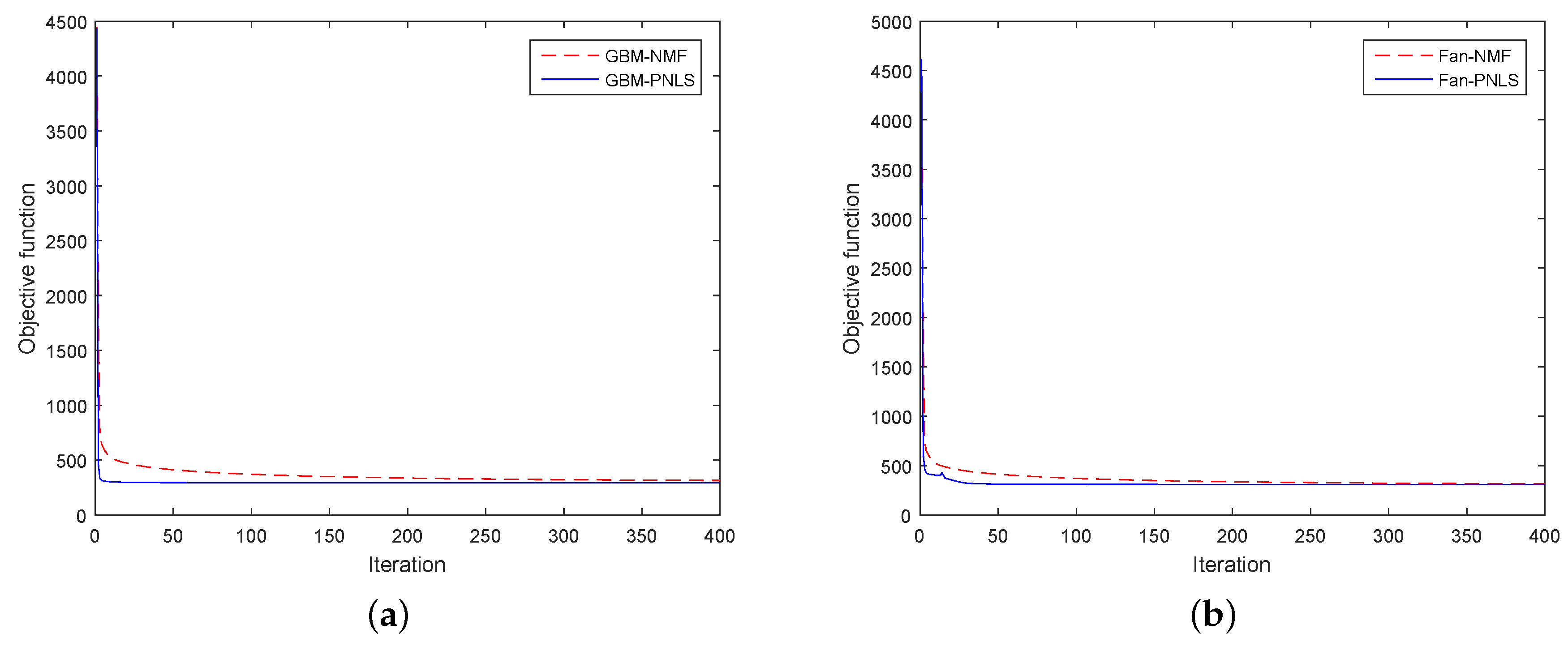
4.1.1. Convergence Test

The test is performed on the synthetic data with five endmembers. The SNR and maximum abundance are set to 30 dB and 0.8, respectively. The proposed GBM-PNLS and the NMF-based GBM-NMF are compared on the GBM data while the proposed Fan-PNLS and the Fan-NMF are compared on the Fan data. Figure 2 shows the convergence paths of the algorithms for the GBM data and the Fan data. One can observe that all the algorithms gradually converge to smaller values as the iteration number increases. However, the proposed PNLS-based algorithms provide faster convergence speed than the other algorithms for both the GBM data and the Fan data. A similar conclusion can be drawn from Figure 3 and Figure 4. The PNLS-based algorithms converge quite quickly for the GBM data and the Fan data and thus the corresponding MSAD and RMSE values decrease rapidly. These results show that the proposed PNLS-based algorithms are more efficient than the NMF-based UNSU algorithms.

4.1.2. Comparison of Different Initialization Methods

In this experiment, we investigate the influence of different initialization strategies. Three methods for the endmember initialization, i.e., random initialization, VCA and SGA, are studied. Due to the randomness of random initialization and VCA, the standard deviations for the results with 20 independent runs are reported. Figure 5 and Figure 6 present the experimental results. One can observe that the proposed PNLS-based algorithms obtain the best unmixing results for the GBM and Fan data no matter which initialization method is used. As expected, the VCA initialization generates results with smaller standard deviations compared with the random initialization. It also can be observed that SGA leads to MSAD and RMSE results slightly better than the average results of VCA’s. In addition, the result of SGA for the same data is deterministic. Therefore, SGA is adopted for the initialization of endmemebers in the following experiments.

4.1.3. Robustness to Various Noise Levels

This experiment examines the algorithms’ robustness to different synthetic images with different noise levels. The endmember number is fixed at 5 and the maximum abundance value is set to 0.8. By varying the SNRs from 20 dB to 40 dB and to infinity (noiseless), 6 synthetic images are generated for the GBM and the Fan model. Figure 7 and Figure 8 show the MSAD and RMSE results for all the algorithms. As expected, the MSADs and RMSEs of all the algorithms degrade when the SNR increases. Over the entire range of the SNRs, the proposed PNLS-based algorithms always obtain the best unmixing results for the GBM and Fan data with the lowest MSAD and RMSE values. For the noise free case, Fan-PNLS performs even worse than other cases, which may be caused by the reason that the proposed algorithm falls into an unsatisfactory local minimum. The two NMF-based nonlinear unmixing methods appear to perform even worse than the standard NMF when it comes to the MSAD. The supervised GBM-based unmixing algorithm (GBM-GDA) also shows a poor performance, even worse than the standard NMF. One possible reason is that the inaccurate endmember estimation provided by the SGA affected the interactions between the endmembers, thereby magnifying the nonlinear mixing error [34]. Actually, a prior knowledge of true endmember is the bias of supervised nonlinear unmixing [16]. From this point of view, the limitations of the supervised nonlinear unmixing algorithms are obvious and the proposed algorithm can eliminate or at least mitigate this limitation.

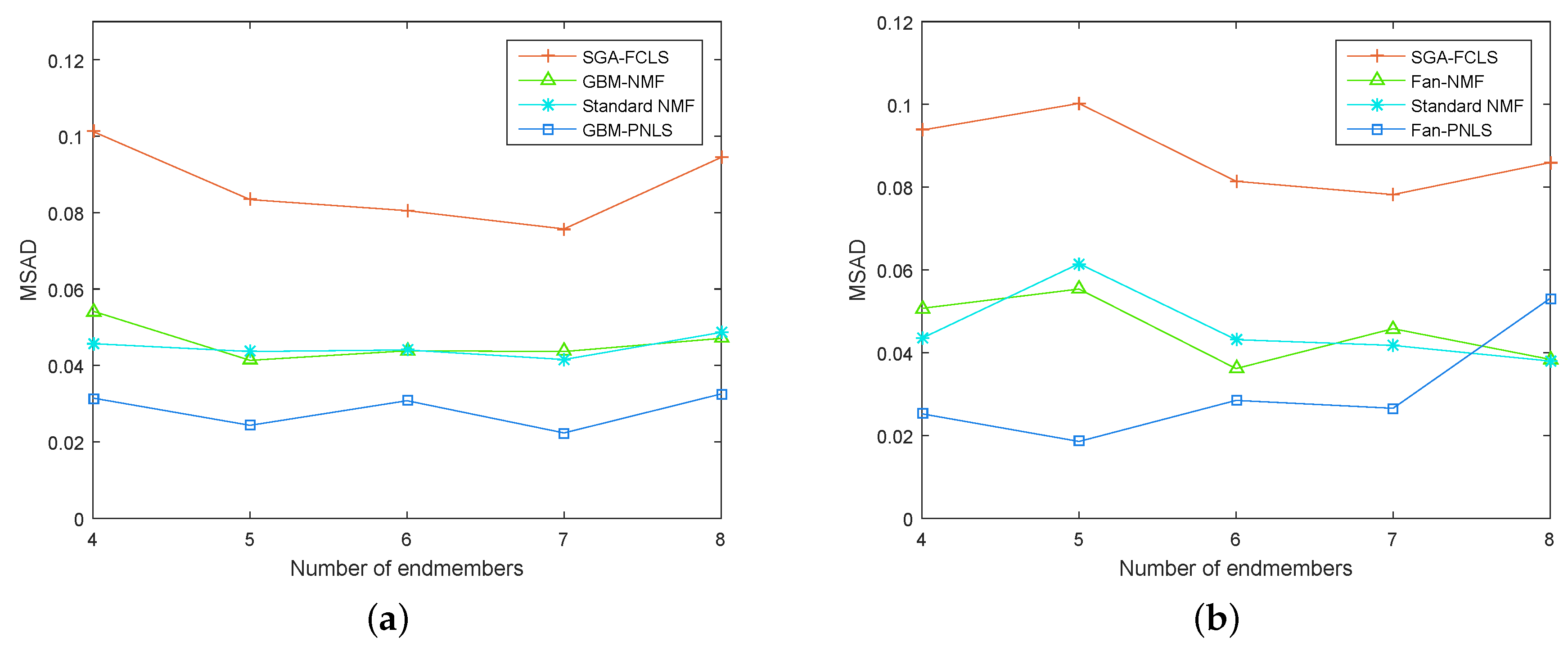
4.1.4. Results for Different Endmember Numbers

The impact of different endmember numbers on the unmixing performance of the proposed algorithm is investigated in this experiment. Six synthetic images are generated with endmember numbers in the range of 3–8 for the GBM and the Fan model. The SNR is fixed to 30 dB and the maximum abundance is set to 0.8. When generating a new image with more endmember number, the spectra used in the previous image are preserved. A new spectrum selected from the USGS library is then added to the endmember set. By this way, we try to eliminate the impact caused by the variation of the endmember class rather than the endmember number. The results are shown in Figure 9 and Figure 10, respectively. The former presents the MSAD results and the latter presents the RMSE results. We can observe that the proposed PNLS-based algorithms are superior to the other methods in most cases with low MSAD and RMSE values for the GBM and Fan data. In some cases, e.g., 8 endmembers, the proposed PNLS achives worse result than the Fan-PNLS and the standard NMF. This may be because the proposed algorithm falls into an unsatisfactory local minimum. It is interesting that the GBM-GDA achives poor results slightly better than the initialization method SGA-FCLS’s. This suggests the limitation of the supervised nonlinear unmixing method again.

4.1.5. Robustness to Different Mixing Degrees

We explore the impact of the mixing degree of the synthetic data in this experiment. The mixing degree can be directly controlled by the maximum abundance value of the data, i.e., larger maximum abundance values correspond to lower mixing degree and vice versa. In this test, the endmember number is fixed to 5 and the SNR is set to 30 dB. The maximum abundance varies from 0.6 to 1 for the evaluation. The experiment results in Figure 11 and Figure 12 show that with the increasing of maximum abundance, the MSAD and RMSE values of all the algorithms decrease generally. This phenomenon mainly results from the fact that the initialization method SGA assumes the presence of pure pixels. More specifically, with increasing maximum abundance, the mixing degree of the data decreases, which leads to the performance improvement of the SGA. The proposed PNLS-based algorithm achives the smallest MSAD or RMSE values in all cases. Moreover, one can observe that the performance of the PNLS is more stable and consistent. The RMSE and MSAD values are comparatively small, even for the smallest maximum abundance value. In contrast, the performance of the GBM-NMF and Fan-NMF is not very satisfactory and decreases obviously when the mixed level increases. The results indicate that the proposed PNLS-based algorithms can handle data with different mixing degrees well, even for the highly mixed data.

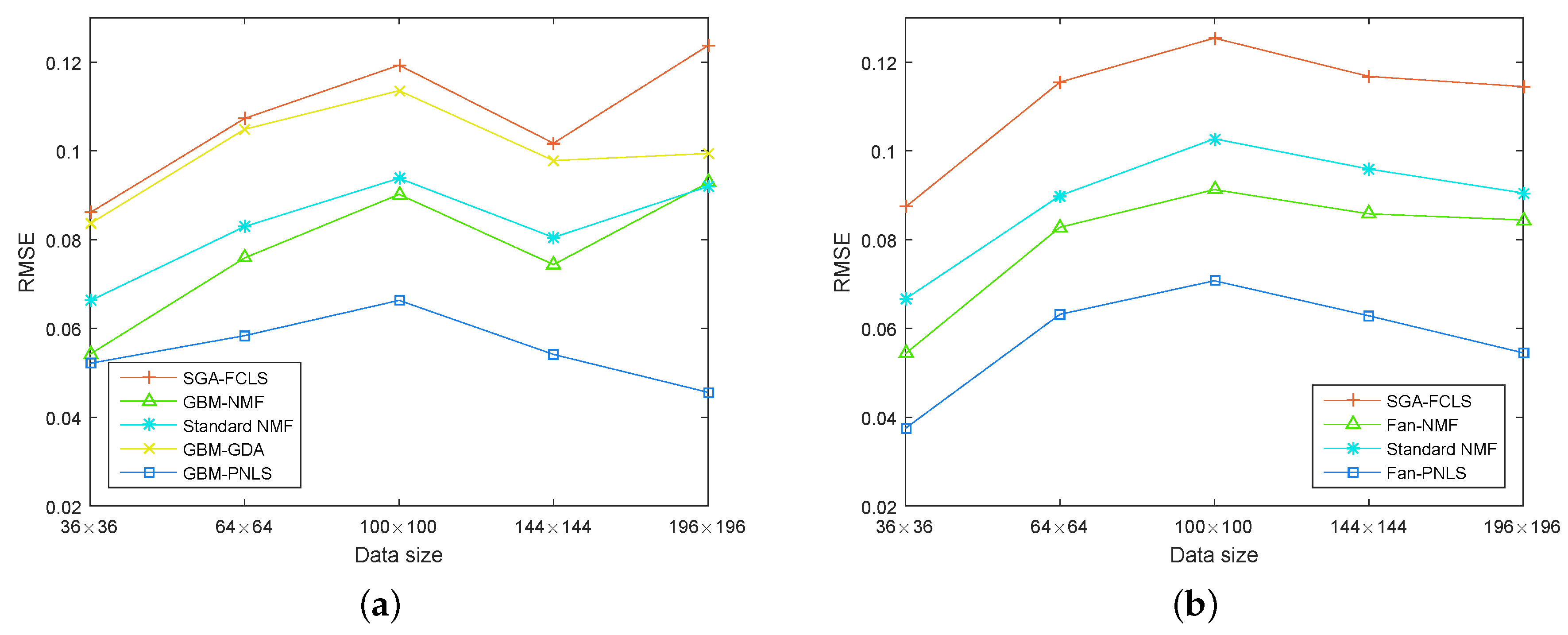
4.1.6. Robustness to Different Data Sizes

In this test, five synthetic images with different sizes are generated for the GBM and the Fan model. The data size is set to 36 × 36, 64 × 64, 100 × 100, 144 × 144, and 196 × 196, respectively. The endmember number is fixed to 5 and the SNR is set to 30 dB. The results in Figure 13 and Figure 14 show that the impact of the data size for all the algorithms. The proposed PNLS-based algorithms always obtain the best estimation accuracy for the GBM data and the Fan data and the performance is quite stable. Meanwhile, the proposed algorithms show more obvious advantage when applied to larger scale of images. Additionly, the performance of the GBM-NMF is unexpectedly worse than that of the standard NMF.

4.2. Real Data Experiments

Jasper Ridge is a dataset widely used in hyperspectral processing, which consists of 512 × 614 pixels. The data includes 224 spectral bands covering the wavelength ranging from 380 nm to 2500 nm with about 10 nm spectral resolution. In this study, we only considered a cropped 100 × 100 sub-scene for simplicity consulting the experiment setup in [35]. Figure 15 shows the 100th band of the scene. After removing the water vapor and atmospheric effects bands, 198 bands remain. According to [35], the endmember number of this sub-scence is set to four, including the substances Road, Soil, Water, and Tree.

Table 3. SADs ($\times {10}^{-2}$) of all the algorithms for the Jasper Ridge data.

Substances	SGA-FCLS	Standard NMF	GBM-NMF	Fan-NMF	GBM-PNLS	Fan-PNLS
Tree	15.59	6.08	16.02	15.88	6.17	5.64
Water	25.40	12.54	26.66	22.73	6.74	7.13
Dirt	13.36	11.51	16.50	49.31	11.84	12.67
Road	10.69	8.71	26.64	23.58	3.31	3.38
Average	16.26	9.71	21.45	27.87	7.02	7.21

quantitatively presents the SAD results for the algorithms involving the endmember estimation for various substances. Compared to the other algorithms, GBM-PNLS and Fan-PNLS obtain better results since all four endmembers are well extracted and the smallest MSAD results are achieved. Figure 16 and Figure 17 show the obtained endmember spectra for the GBM-PNLS and Fan-PNLS algorithms, as well as the reference spectra. The extracted endmembers and the reference endmembers are nearly identical. Since the ground truth of abundance map is not available, reference data have been often used as the benchmark to evaluate the accuracy of algorithms. It’s worth noting that the accuracy of reference data is unknown actually [36]. In this paper, we use the reference abundance maps obtained from [37] to further evaluate the algorithms’ performance. The reference data have been commonly used in [35,38].

Table 4. RMSEs ($\times {10}^{-2}$) of all the algorithms for the Jasper Ridge data.

	SGA-FCLS	Standard NMF	GBM-GDA	GBM-NMF	Fan-NMF	GBM-PNLS	Fan-PNLS
RMSE	38.38	15.51	37.54	21.80	24.70	14.78	14.65

presents the RMSE performance of different algorithms. We can also find that the proposed metohds’ results are generally better than those yielded by the other algorithms. It is interesting that the two PNLS-based algorithms perform quite similarly. This reflects the similar modeling capability of the GBM and Fan model. Figure 18 shows the corresponding abundance maps achieved by different algorithms, as well as the reference maps. Through visual comparison, we can find that the proposed proposed GBM-PNLS and Fan-PNLS achieve abundance maps that are more consistent with the reference maps compared with other methods. To further investigate the nonlinear behavior of proposed method, the maps of nonlinearity coefficients obtained by the proposed GBM-PNLS are provided in Figure 19. As shown in the figure, the bilinear mixing effect mainly exists in the transition regions of different substances, which accords with the physical truth well. Figure 19b shows that a large bilinear spectral mixing effect exists in the mixing regions of tree and soil since there exist 3-D multilayered structures and multiple scattering is a common phenomenon in these regions. It can also be observed that the bilinear mixing effect appears in the boundary of water and soil, as well as the boundary of road and soil, which is also consistent with physical model of GBM-based unmixing. The above results demonstrate that the proposed methods have potential in exploring underlying nonlinear effects and handling BMM-based spectral unmixing.

5. Conclusions

In this study, two PNLS-based UNSU algorithms are proposed for the GBM and Fan model. They are able to obtain the endmembers, abundances and nonlinearity coefficients simultaneously in a complete iteration. To better achieve the unsupervised unmixing task, the proposed algorithms integrate a Sigmoid parameterization so that the nonnegative constraint and nonlinearity coefficients boundary constraint can be relaxed. The optimization problem of the UNSU is then transformed into two or three alternate PNLS problems which can be solved by the Gauss–Newton method. Compared to existing NMF-based UNSU methods, the PNLS-based UNSU algorithms converge faster and the performance is improved to a certain extent. We evaluate the performance of the proposed algorithms on both synthetic and real data. The experimental results show that the proposed algorithms possess better unmixing performance than the other reference algorithms.

There are still some issues to resolve. For example, the computational complexity is still high, especially when the dataset is large. Considering the proposed algorithms are actually highly parallel, hopefully, the computational complexity can be reduced using high-performance computing such as graphic processing unit (GPU) acceleration, which will be explored in a further study.

References

1. Nascimento, J.M.P.; Dias, J.M.B. Vertex component analysis: A fast algorithm to unmix hyperspectral data. IEEE Trans. Geosci. Remote Sens. 2005, 43, 898–910. [Google Scholar] [CrossRef]
2. Heinz, D.C.; Chang, C. Fully constrained least squares linear spectral mixture analysis method for material quantification in hyperspectral imagery. IEEE Trans. Geosci. Remote Sens. 2002, 39, 529–545. [Google Scholar] [CrossRef]
3. Lee, D.D.; Seung, H.S. Learning the parts of objects by non-negative matrix factorization. Nature 1999, 401, 788–791. [Google Scholar] [CrossRef] [PubMed]
4. Liu, X.; Xia, W.; Wang, B.; Zhang, L. An approach based on constrained nonnegative matrix factorization to unmix hyperspectral data. IEEE Trans. Geosci. Remote Sens. 2011, 49, 757–772. [Google Scholar] [CrossRef]
5. Lu, X.; Wu, H.; Yuan, Y. Double constrained NMF for hyperspectral unmixing. IEEE Trans. Geosci. Remote Sens. 2014, 52, 2746–2758. [Google Scholar] [CrossRef]
6. Heylen, R.; Parente, M.; Gader, P. A review of nonlinear hyperspectral unmixing methods. IEEE J. Sel. Top. Appl. Earth Obs. Remote Sens. 2014, 7, 1844–1868. [Google Scholar] [CrossRef]
7. Kwon, H.; Nasrabadi, N.M. Kernel orthogonal subspace projection for hyperspectral signal classification. IEEE Trans. Geosci. Remote Sens. 2005, 43, 2952–2962. [Google Scholar] [CrossRef]
8. Chen, J.; Richard, C.; Honeine, P. Nonlinear unmixing of hyperspectral data based on a linear-mixture/nonlinear-fluctuation model. IEEE Trans. Signal Process. 2013, 61, 480–492. [Google Scholar] [CrossRef]
9. Gu, Y.; Wang, S.; Jia, X. Spectral unmixing in multiple-kernel Hilbert space for hyperspectral imagery. IEEE Trans. Geosci. Remote Sens. 2013, 51, 3968–3981. [Google Scholar] [CrossRef]
10. Hapke, B. Bidirectional reflectance spectroscopy: 1. Theory. J. Geophys. Res. Solid Earth 1981, 86, 3039–3054. [Google Scholar] [CrossRef]
11. Babaie-Zadeh, M.; Jutten, C.; Nayebi, K. Blind separating convolutive post-nonlinear mixtures. In Proceedings of the ICA 2001, San Diego, CA, USA, December 2001; pp. 138–143. [Google Scholar]
12. Nascimento, J.M.P.; Bioucasdias, J.M. Nonlinear mixture model for hyperspectral unmixing. In Proceedings Image and Signal Processing for Remote Sensing XV. International Society for Optics and Photonics; SPIE: Berlin, Germany, 2009; Volume 7477, p. 74770I. [Google Scholar]
13. Fan, W.; Hu, B.; Miller, J.; Li, M. Comparative study between a new nonlinear model and common linear model for analysing laboratory simulated-forest hyperspectral data. Int. J. Remote Sens. 2009, 30, 2951–2962. [Google Scholar] [CrossRef]
14. Halimi, A.; Altmann, Y.; Dobigeon, N.; Tourneret, J.Y. Unmixing hyperspectral images using the generalized bilinear model. In Proceedings of the IEEE International Geoscience and Remote Sensing Symposium, Vancouver, BC, Canada, 24–29 July 2011; pp. 1886–1889. [Google Scholar]
15. Altmann, Y.; Halimi, A.; Dobigeon, N.; Tourneret, J.Y. Supervised nonlinear spectral unmixing using a postnonlinear mixing model for hyperspectral imagery. IEEE Trans. Image Process. 2012, 21, 3017–3025. [Google Scholar] [CrossRef] [PubMed]
16. Yokoya, N.; Chanussot, J.; Iwasaki, A. Nonlinear unmixing of hyperspectral data using semi-nonnegative matrix factorization. IEEE Trans. Geosci. Remote Sens. 2014, 52, 1430–1437. [Google Scholar] [CrossRef]
17. Boardman, J.W. Automating spectral unmixing of AVIRIS data using convex geometry concepts. In Proceedings of the Summaries of the Fourth Annual JPL Airborne Geoscience Workshop, Washington, DC, USA, 25–29 October 1993. [Google Scholar]
18. Chang, C.I.; Wu, C.C.; Liu, W.; Ouyang, Y.C. A new growing method for simplex-based endmember extraction algorithm. IEEE Trans. Geosci. Remote Sens. 2006, 44, 2804–2819. [Google Scholar] [CrossRef]
19. Winter, M.E. N-FINDR: An algorithm for fast autonomous spectral end-member determination in hyperspectral data. In Proceedings Imaging Spectrometry V. International Society for Optics and Photonics; SPIE: Berlin, Germany, 1999; Volume 3753, pp. 266–276. [Google Scholar]
20. Altmann, Y.; Dobigeon, N.; Tourneret, J.Y. Unsupervised post-nonlinear unmixing of hyperspectral images using a Hamiltonian Monte Carlo algorithm. IEEE Trans. Image Process. 2014, 23, 2663–2675. [Google Scholar] [CrossRef]
21. Eches, O.; Guillaume, M. A bilinear–bilinear nonnegative matrix factorization method for hyperspectral unmixing. IEEE Geosci. Remote Sens. Lett. 2013, 11, 778–782. [Google Scholar] [CrossRef]
22. Li, J.; Li, X.; Zhao, L. Unsupervised nonlinear hyperspectral unmixing based on the generalized bilinear model. In Proceedings of the IEEE International Geoscience and Remote Sensing Symposium, Beijing, China, 10–15 July 2016; pp. 6553–6556. [Google Scholar]
23. Lin, C.J. Projected gradient methods for nonnegative matrix factorization. Neural Comput. 2007, 19, 2756–2779. [Google Scholar] [CrossRef]
24. Lee, D.D.; Seung, H.S. Algorithms for non-negative matrix factorization. In Proceedings of the International Conference on Neural Information Processing Systems, Denver, CO, USA, 3–8 December 2001; pp. 556–562. [Google Scholar]
25. Bro, R.; De Jong, S. A fast non-negativity-constrained least squares algorithm. J. Chemom. 2015, 11, 393–401. [Google Scholar] [CrossRef]
26. Kim, H.; Park, H. Nonnegative matrix factorization based on alternating nonnegativity constrained least squares and active set method. Siam J. Matrix Anal. Appl. 2008, 30, 713–730. [Google Scholar] [CrossRef]
27. Han, J.; Moraga, C. The Influence of the Sigmoid Function Parameters on the Speed of Backpropagation Learning; Springer: Berlin/Heidelberg, Germany, 1995; pp. 195–201. [Google Scholar]
28. Björck, Å. Numerical Methods for Least Squares Problems; SIAM: Philadelphia, PA, USA, 1996. [Google Scholar]
29. Levenberg, K. A method for the solution of certain non-linear problems in least squares. J. Heart Lung Transpl. Off. Publ. Int. Soc. Heart Transpl. 1944, 31, 436–438. [Google Scholar] [CrossRef]
30. Halimi, A.; Altmann, Y.; Dobigeon, N.; Tourneret, J.Y. Nonlinear Unmixing of Hyperspectral Images Using a Generalized Bilinear Model. IEEE Trans. Geosci. Remote Sens. 2011, 49, 4153–4162. [Google Scholar] [CrossRef] [Green Version]
31. Zdunek, R. Hyperspectral image unmixing with nonnegative matrix factorization. In Proceedings of the International Conference on Signals and Electronic Systems, Wroclaw, Poland, 18–21 September 2012; pp. 1–4. [Google Scholar]
32. Drees, L.; Roscher, R.; Wenzel, S. Archetypal Analysis for Sparse Representation-based Hyperspectral Sub-pixel Quantification. Photogramm. Eng. Remote Sens. 2018, 84, 279–286. [Google Scholar] [CrossRef]
33. Swayze, G.A.; Clark, R.N.; King, T.V.V.; Gallagher, A.; Calvin, W.M. The U.S. Geological Survey, Digital Spectral Library: Version 1: 0.2 to 3.0 μm; Technical Report; Geological Survey (US): Reston, VA, USA, 1993.
34. Pu, H.; Chen, Z.; Wang, B.; Xia, W. Constrained least squares algorithms for nonlinear unmixing of hyperspectral imagery. IEEE Trans. Geosci. Remote Sens. 2014, 53, 1287–1303. [Google Scholar] [CrossRef]
35. Zhu, F.; Wang, Y.; Xiang, S.; Fan, B.; Pan, C. Structured sparse method for hyperspectral unmixing. ISPRS J. Photogramm. Remote Sens. 2014, 88, 101–118. [Google Scholar] [CrossRef]
36. Williams, M.D.; Kerekes, J.P.; van Aardt, J. Application of abundance map reference data for spectral unmixing. Remote Sens. 2017, 9, 793. [Google Scholar] [CrossRef]
37. Zhu, F. Hyperspectral Unmixing Datasets & Ground Truths. 2014. Available online: http://www.escience.cn/people/feiyunZHU/DatasetGT.html (accessed on 5 June 2017).
38. Wang, Y.; Pan, C.; Xiang, S.; Zhu, F. Robust hyperspectral unmixing with correntropy-based metric. IEEE Trans. Image Process. 2015, 24, 4027–4040. [Google Scholar] [CrossRef] [PubMed]
Figure 1. Spectra from the USGS library: (a) Carnallite NMNH98011 (b) Ammonioalunite NMNH145596 (c) Biotite HS28.3B (d) Actinolite NMNHR16485 (e) Almandine WS478 (f) Ammonio-jarosite SCR-NHJ.
Remotesensing 11 00148 g001
Figure 2. Objective function versus number of iteration: (a) GBM-PNLS and GBM-NMF for GBM data, (b) Fan-PNLS and Fan-NMF for Fan data.
Remotesensing 11 00148 g002
Figure 3. MSAD versus number of iteration: (a) GBM-PNLS and GBM-NMF for GBM data, (b) Fan-PNLS and Fan-NMF for Fan data.
Remotesensing 11 00148 g003
Figure 4. RMSE versus number of iteration: (a) GBM-PNLS and GBM-NMF for GBM data, (b) Fan-PNLS and Fan-NMF for Fan data.
Remotesensing 11 00148 g004
Figure 5. MSAD results for different initialization methods for: (a) GBM data, (b) Fan data.
Remotesensing 11 00148 g005
Figure 6. MSAD results for different initialization methods for: (a) GBM data, (b) Fan data.
Remotesensing 11 00148 g006
Figure 7. MSAD results for different SNRs for: (a) GBM data, (b) Fan data.
Remotesensing 11 00148 g007
Figure 8. RMSE results for different SNRs for: (a) GBM data, (b) Fan data.
Remotesensing 11 00148 g008
Figure 9. MSAD results for various numbers of endmembers for: (a) GBM data, (b) Fan data.
Remotesensing 11 00148 g009
Figure 10. RMSE results for various numbers of endmembers for: (a) GBM data, (b) Fan data.
Remotesensing 11 00148 g010
Figure 11. MSAD results for different mixing degrees for: (a) GBM data, (b) Fan data.
Remotesensing 11 00148 g011
Figure 12. RMSE results for different mixing degrees for: (a) GBM data, (b) Fan data.
Remotesensing 11 00148 g012
Figure 13. MSAD results for different data sizes for: (a) GBM data, (b) Fan data.
Remotesensing 11 00148 g013
Figure 14. RMSE results for different data sizes for: (a) GBM data, (b) Fan data.
Remotesensing 11 00148 g014
Figure 15. The 100th band of the Jasper Ridge data.
Remotesensing 11 00148 g015
Figure 16. Comparison of the USGS library spectra (solid green line) with the endmembers extracted by GBM-PNLS (red dotted line) on the Jasper Ridge data: (a) Tree, (b) Water, (c) Soil, (d) Road.
Remotesensing 11 00148 g016
Figure 17. Comparison of the USGS library spectra (solid green line) with the endmembers extracted by Fan-PNLS (red dotted line) on the Jasper Ridge data: (a) Tree, (b) Water, (c) Soil, (d) Road.
Remotesensing 11 00148 g017
Figure 18. Abundance maps of the Jasper Ridge data by the reference data, SGA-FCLS, Standard NMF, GBM-GDA, GBM-NMF, Fan-NMF, GBM-PNLS and Fan-PNLS, respectively, from top to bottom. Each column shows the corresponding abundance maps of a same endmember.
Remotesensing 11 00148 g018
Figure 19. Nonlinearity coefficients maps of B obtained by the proposed GBM-PNLS for the Jasper Ridge data: (a) Tree-Water, (b) Tree-Soil, (c) Tree-Road, (d) Water-Soil, (e) Water-Road, (f) Soil-Road.
Remotesensing 11 00148 g019