Article

Investigative Spatial Distribution and Modelling of Existing and Future Urban Land Changes and Its Impact on Urbanization and Economy

1
Department of Civil Engineering, COMSATS University Islamabad, Abbottabad Campus, University Road, 22060 Abbottabad, KPK, Pakistan
2
Department of Geomatics Engineering, Schulich School of Engineering, The University of Calgary, 2500 University Drive NW Calgary, Calgary, AB T2N 1N4, Canada
3
Advanced & Latest Informatics (ALI) Inc., 848 N. Rainbow Blvd., #3529, Las Vegas, NV 89107, USA
4
The Urban Unit, Shaheen Complex, 503 Edgerton Rd Lahore, Punjab 54000, Pakistan
*
Author to whom correspondence should be addressed.
Remote Sens. 2019, 11(2), 105; https://doi.org/10.3390/rs11020105
Submission received: 15 October 2018 / Revised: 4 January 2019 / Accepted: 6 January 2019 / Published: 9 January 2019

Abstract

:
Land use and land cover (LULC) change analysis is a critical instrument for studying urban growth across the world. Our objectives were to produce historical LULC maps during the 1988–2016 period for spatial and temporal analysis, forecast future LULC until 2040 by using the Markov model, and identify the impact of LULC on urbanization. Two scenes of Landsat-5 TM for 1988 and 2001 and one scene of Landsat-8 OLI for 2016 were processed and used. The Normalized Difference Vegetation Index (NDVI) model with precise class value ranges was applied to produce land cover maps with six classes of water, built-up, barren land, shrub and grassland, sparse vegetation, and dense vegetation. LULC maps for the years of 1988 and 2001 were used to develop an LULC transformation matrix. It was used to drive an LULC transformation probability matrix using a Markov model for future forecasting of LULC in 2014, 2027, and 2040. The accuracy of 2016 LULC classes was estimated by comparing it against Markov modeled classes. It was found that the areas for: (i) water decreased from 1.43% to 0.51%; (ii) built-up increased from 9.58% to 20.80%; (iii) barren land decreased from 29.50% to 13.40%; (iv) shrub and grass land decreased from 30.57% to 21.10%; (v) sparse vegetation increased from 18% to 20.10%; and (vi) dense vegetation increased from 10.57% to 24.10%. The variations in LULC classes could be noticed by 2040 as compared to 1988. This LULC variation revealed that the water could decrease to 5.32 km2 from 25.37 km2; the built-up could increase to 625.16 km2 from 168.29 km2; the barren land could decrease to 137.53 km2 from 514.13 km2; the shrub and grassland could decrease to 297.68 km2 from 539.46 km2; the sparse vegetation could decrease to 297.68 km2 from 539.46 km2; and the dense vegetation could increase to 409.65 km2 from 191.51 km2. The LULC classification accuracy was 90.27% and 95.11% for 1988 and 2001, respectively. The co-efficient of determination (R2) was found to be 0.90 for 2016 LULC classes obtained from Landsat-8 and derived from a Markov model. For District Lahore, the LULC changes could be related to increasing population and intense migration trends, which had progressive impact on infrastructure development, industrial and economic growth, and detrimental effects on water resources.

1. Introduction

Land use and land cover (LULC) change analysis provides useful information for studying the urban land changes for growing cities of the world [1,2,3]. Lahore is a rapidly developing economic hub of Pakistan, which faces many challenges that include: (i) population increase; (ii) infrastructure development; (iii) road construction; (iv) rising transportation; (v) urban built-up sprawl; (iv) pressure on natural resources; (v) natural hazards; and (vi) climatic changes. Urban growth leads to land development, industrialization, and urbanization, but creates problems related to population, traffic, and environmental degradation [4].
These challenging factors have effects on past, current, and future urban land in terms of urbanization and economic activities. It is therefore important to use historical satellite data using remote sensing techniques and an authentic model for future forecasting of LULC [5,6]. The major premise of change detection through remote sensing is that it can identify the aberrant and normal transitions in land cover between two or more dates [7]. Remote sensing data is extremely useful due to its repetitive coverage, synoptic view and real time data acquisition. Digital data of satellite images can accurately compute LULC classes. It aids in maintaining spatial infrastructure, which is profoundly required to monitor urban expansion and land use transitions. Monitoring and modeling of spatial data has become a trend, in order to satisfy the need of policy makers and planners for precisely and accurately achieving LULC information [8]. There are different indices, which were developed for LULC mapping and analysis. For example, the normalized difference vegetation index (NDVI) [9], soil-adjusted vegetation index (SAVI) [10], normalized difference built-up index (NDBI) [11], and an indexed-based built-up index (IBI) [12]. The latest techniques were also developed recently for quantifying land cover changes (e.g., modified change vector approach by Xu et al.) [13]. In addition, image classification techniques, such as maximum likelihood approach, Random Forest (RF), k-Nearest Neighbor (kNN), and Support Vector Machine (SVM) were also employed [14,15]. For understanding future scenarios of LULC, different statistical and mathematical models were used. Among them, a Markov model was widely utilized [16,17].
Some studies were accomplished to conduct LULC changes and performed spatio-temporal analysis by considering historical trends as well as forecast future LULC. A study was completed for Bangladesh to predict LULC during 2010–2030 using formerly developed Dynamics of Land Systems models on the basis of land use maps (30 m resolution) obtained from China Globe Cover and affecting factors of geophysical, climatic, proximity, and socioeconomic. The findings indicated a decline of cultivated land and increase in built-up area. The future scenarios indicated increases in forest area and grassland under ecological protection, with expansion in built-up areas under economic growth [16]. In another study, spatio-temporal variability was obtained during 1998–2006 using Indian Remote Sensing Satellite (IRS) images, and a Markov model was used to predict future spatial distribution of land for 2014 and 2022 for Tiruchirappalli city of India. The results indicated an increase in built-up area and a decrease in waste land [17]. A Land Transformation Model coupled with geographic information systems (GIS) and artificial neural networks was used for forecasting LULC in Michigan’s Grand Traverse Bay Watershed in the United States. The land use data was obtained from Michigan Resource Information System (1:24,000 aerial photography of 1980). The land use change pattern was understood at different scales and relative effect of site and situation variables were identified [18]. The simulation of land use spatial patterns of towns and villages were accomplished for 2001, 2006, and 2008 on the basis of land use data for Fangshan district of Beijing, China. Cellular Automata and the Markov model were used for simulating the spatial pattern of land use in 2015. Overall, the results were satisfactory and the land use classes could preserve their changes [19]. The scenario simulation and the prediction of LULC change in Beijing, China was accomplished by using a CLUE-S model with a Markov model for 2010 to 2020. The driving factors in this study were related to land-adaptive, regional spatial, and socio-economic. It was found that the cultivated land could be converted into urban built-up land in the future [20]. The urban growth and urban living environment were simulated by using a logistic regression model for Jeju and Chuncheon of South Korea, and the driving factors were topography, economy, society, and environment. The results indicated a continuous increase in built-up area and surface temperature by 2025 [21].
In Lahore, rapid economic growth has led to urbanization, which changed the usage of existing land and it also built pressure on the available resources. The increase in population, better economy, and proximity of inhabitants to basic facilities and resources are the potential factors for urban sprawl. It resulted in greater land utilization and disintegration of natural and man-made features [22]. Due to all these factors, District Lahore was selected for studying the land cover change analysis. In this paper, our objectives were to: (i) produce historical LULC maps during the 1988–2016 period for spatial and temporal analysis; (ii) forecast future LULC until 2040 by using a Markov model; and (iii) identify the impact of LULC on urbanization.

2. Study Area and Data
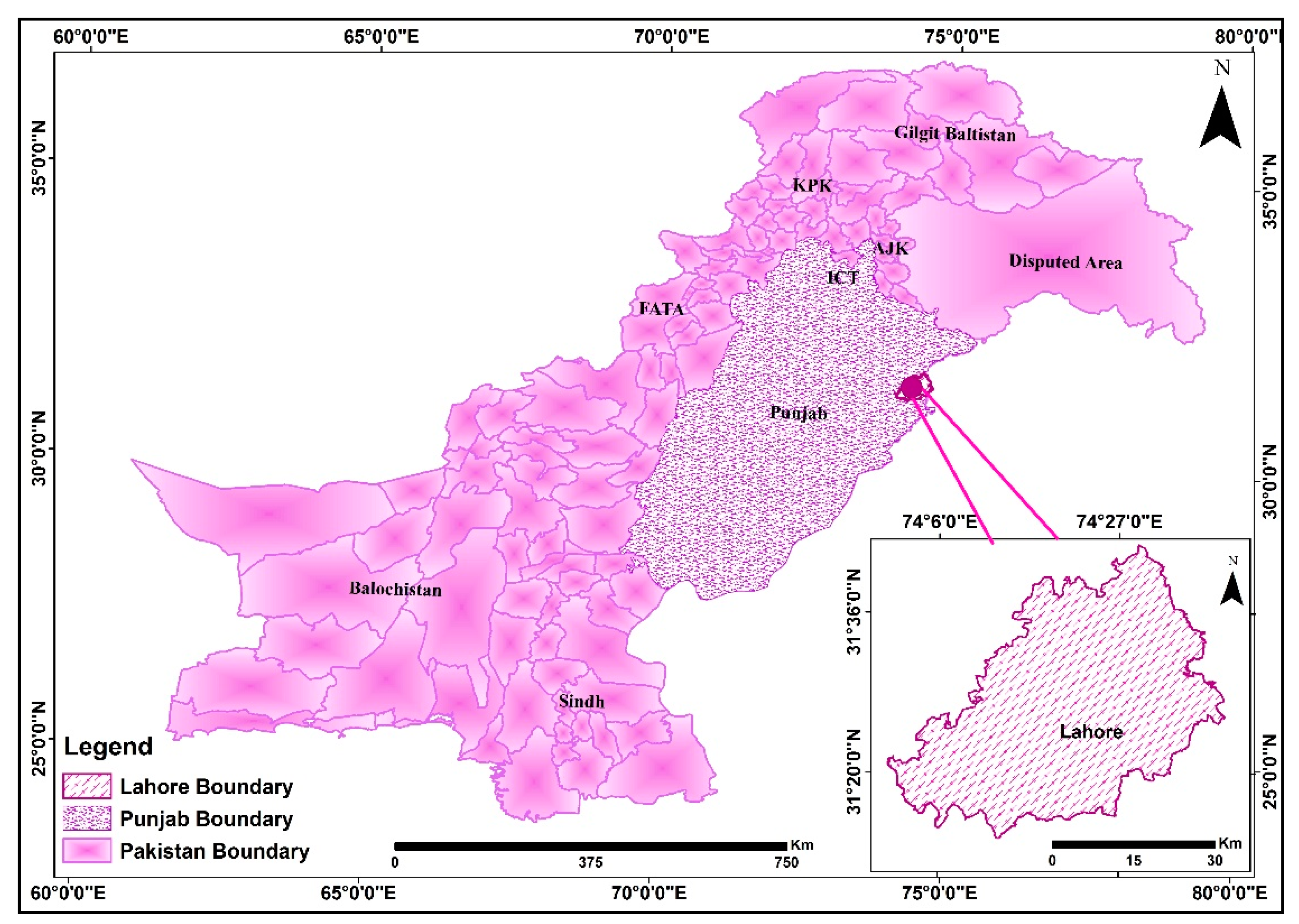
2.1. Study Area

The study area (District Lahore) is located in the north-eastern side of Punjab province of Pakistan, as shown in Figure 1. It is the capital of the province and the second largest city in the country with a total area of 1772 km2 [23]. The climate of the study area is semi-arid. The mean annual temperature ranges from 13.09 °C to 24.71 °C in winter and from 25.73 °C to 36.09 °C in summer. The mean annual precipitation varies from 88.28 mm in summer to 17.04 mm in winter. The major river flowing through study area is River Ravi, which originates from the Himalayan region. Lahore city has a flat slope with a general altitude of 208 to 213 m [23]. The total population of the district of Lahore in 2017 is almost 11.12 million [24].

2.2. Satellite Image Acquisition

Three scenes of Landsat satellite imageries were used for different dates during the period of 1988–2016, which were: (i) Landsat-5 TM multispectral image acquired on November 5, 1988; (ii) Landsat-5 TM multispectral image acquired on September 22, 2001; and (iii) Landsat-8 OLI multispectral image acquired on October 17, 2016. The intent was to use images at 10-year intervals, however, the effort was given to select cloud-free images that were acquired during the same season. The approximate sizes of images are 183 km × 170 km and 185 km × 172 km, respectively. The spectral bands used in this study were red (R) and near infrared (NIR). The temporal resolution is 16 days and the spatial resolution is 30 m for both types of satellites. All the scenes utilized in this study were obtained from GLOVIS in GeoTIFF format with the Level 1T correction, which includes the radiometric, geometric, and topographic accuracies. The projection for all satellites was Universal Transverse Mercator (UTM). In addition, the Google Earth images (during 2001 and 2016) and digital topographic map of 1988, available from Urban Unit of the Punjab Government, were used to aid the process of generating the LULC maps during the 1988–2016 period. In particular, the 2011 Google Earth Images and 1988 digital topographic map were used to acquire ground sample plots for validation purposes, as no other alternative was available in our hand.

3. Methods

3.1. Satellite Image Pre-Processing

The satellite images were processed for classification in this study. The different mathematical models used in processing of the satellite imagery were obtained from Landsat 7 Science Data Users Handbook [25]. The digital number values of Landsat-5 TM imagery were converted into planetary reflectance for red and near infrared spectral bands, using the model given in Landsat 7 Science Data Users Handbook [25]. In this process, the model required the following parameters: (i) minimum and maximum quantized calibrated pixel values; (ii) spectral radiance scaled to minimum and maximum quantized calibrated pixel values; (iii) earth–sun distance; (iv) mean solar exo-atmospheric irradiance values; and (v) solar zenith angle. All of the parameters were available from metadata files of satellite imageries; except for the earth-sun distance, available from Landsat 7 Science Data Users Handbook [25] and solar exo-atmospheric irradiance values, available from Chander and Markham [26]. For Landsat-8 OLI images, the model given in Landsat 8 Science Data Users Handbook [27] was used for transforming the digital number values into planetary reflectance. In this case, the required parameters were: (i) multiplicative rescaling factor; (ii) additive rescaling factor; and (iii) solar elevation angle; where all of them were available from metadata files.
The images acquired at different times have different atmospheric conditions and view angles. In order to make these temporal images spectrally resemble each other, Dark Object Subtraction correction was applied, using an equation as given in Landsat 8 Data User Handbook [27]. The different input parameters required in this equation were path radiance, band-specific multiplicative rescaling factor, and band-specific additive rescaling. The values for all these parameters were obtained from the metadata of the satellite images.
Upon accomplishing the above steps, we opted to generate NDVI images using the Landsat images acquired in 1988, 2001, and 2016 using the following expression [9]:
NDVI = ρ N I R ρ R ρ N I R + ρ R
where, ρ is the surface reflectance-values for the near infrared (NIR) and red (R) spectral bands.

3.2. Development of LULC Maps and Spatio-Temporal Analysis

The classes of land cover were: (i) water; (ii) built-up; (iii) barren land; (iv) shrub and grass land; (v) sparse vegetation; and (vi) dense vegetation. In this study, six major classes were considered. As these were the main classes where land cover changes and transitions were noticed for the last few decades. In another research for Lahore, five classes were taken which incorporates built-up, vegetation, open area, water bodies and mixed class [28]. The further classification was only possible with sparse and dense vegetation by further classifying them into different types of crop classes. For crop classification, training data set was required through extensive field survey, which was not possible for previous years (i.e., 1988, 2001 and 2016). Due to these factors, only six land cover classes were possible which were considered in this study.
In generating the LULC map, we opted to adapt an NDVI-based classification method, as recommended by U.S. Geological Services (USGS) [29], due to its simplicity. Also, NDVI has been used for various classification schemes in recent times [30,31,32,33]. As a first step, we considered the 2016 NDVI image that was arbitrarily divided into 80 classes. Then, we used the 300 sample plots and Google Earth images of 2016 in order to merge or divide these classes, which eventually resulted in the final six LULC classes. Consequently, we generated the LULC class-specific NVDI ranges upon exploiting the 2016 NDVI image, which was then applied over both of the 2001 and 1988 NDVI images. As the 2016 NDVI image was used for calibration purposes, we therefore opted to use both 2001 and 1998-derived LULC maps for validation. In doing so, we acquired 1800 sample plots for each of the years 2001 and 1988, based on visual interpretation of “Google Earth images of 2001” and “digital topographic map of 1988”. Finally, the confusion matrices were generated in order to demonstrate the effectiveness of our adapted method.
The areas for LULC classes were calculated in km2 and percentages for the years 1988, 2001, and 2016 using LULC maps. The classes were compared with each other, both for the same years and in different years. The graphs and maps were developed to show the spatial and temporal LULC changes.

3.3. Future Prediction of LULC Changes

A transformation matrix is the means to define quantities of transformations from a specific land cover to another land cover category at a later date. LULC maps for the years of 1988 and 2001 were used to develop an LULC transformation matrix. This matrix provided us the transformation of each LULC class for the year 1988 into six classes for the year 2001. A Markov model was applied for development of a transformation probability matrix and predicting future changes for LULC. A Markov Model is a useful tool for simulating LULC changes. It helps to predict future changes on the basis of current data. A Markov model was used in many studies [16,17,19,34]. The accuracy of Markov models were verified in some studies [19,35]. On the basis of the LULC transformation matrix developed, an LULC transformation probability matrix was derived using a Markov Model during the period 1988–2001. It was assumed that the probability of changes for built-up class to other classes is zero. This assumption is considered on the basis that the built-up areas cannot be converted into any other LULC class [17]. This model was applied to analyze LULC changes from one period (1988) to another period (2001), which was made basis of projecting future LULC changes for 2014, 2027, and 2040 at the same interval of 13 years. A comparison was made between the LULC areas of classes obtained from Landsat-8 and Markov model for the year 2016. The model values for year the 2016 were achieved by linear interpolation of the model projected-values between the years of 2014 and 2027. The co-efficient of determination (R2) was finally calculated by plotting modeled and Landsat-8 extracted values on a linear graph.
Note that our aim was to use Landsat images at 10-year intervals, however, the effort was given to select cloud-free images that were acquired during the same season. As a result, we found useful images at 13-year intervals. Consequently, we used 13-year intervals for implementing the Markov Chain Model.

4. Results

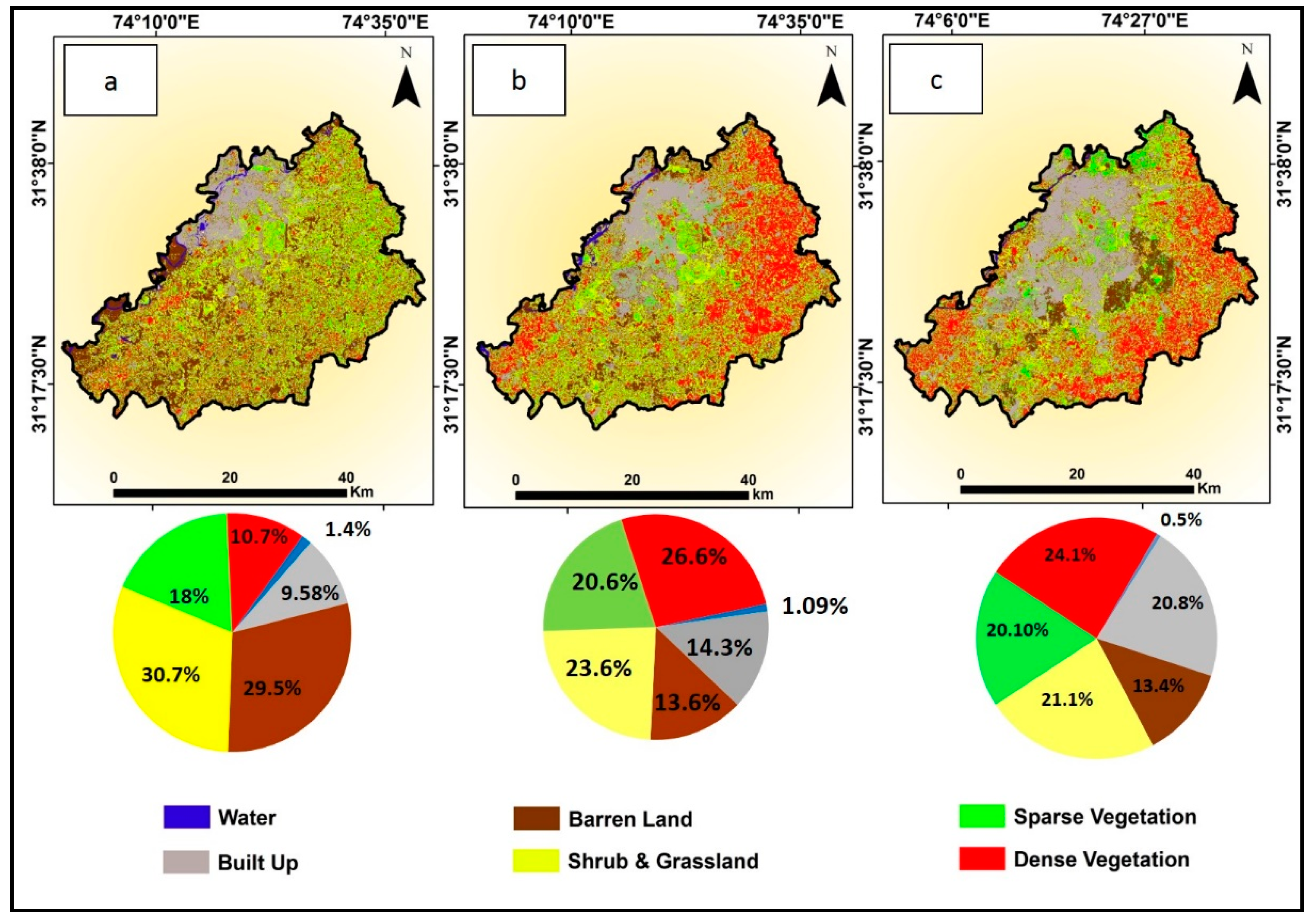
4.1. Land Cover Classification and Spatio-Temporal Analysis

On the basis of the methodology described in Section 3.2, precise NDVI value ranges for six LULC classes derived from the 2016 Landsat-8 OLI image are provided in Table 1. Upon implementing these NDVI ranges, we generated the 1988 and 2001 LULC maps and evaluated them against the 1800 sample plots in each of the events, as reported in Table 2 and Table 3.
The overall accuracy was 90.27% for the 1988 LULC map and it was 95.11% for 2001. The Kappa statistics were 0.88 and 0.94 for 1988 and 2001, respectively. From Table 2, it is obvious that in the case of 1988, according to the producer’s accuracy, the percentages of accuracy were 93.33%, 90%, 87%, 96%, 83.33%, and 92.33% for water bodies, built up, barren land, shrub and grassland, sparse vegetation, and dense vegetation, respectively. The percentages for user’s accuracy were 100%, 85.12%, 86%, 90.03%, 92.59%, and 89.64% for LULC classes, respectively. For 2001, Table 3 presents the percentages of producer’s accuracy as 97.3%, 92%, 94%, 96%, 94.66%, and 96.66% for water bodies, built up, barren land, shrub and grassland, sparse vegetation, and dense vegetation, respectively. The percentages for user’s accuracy were 100%, 96.15%, 88%, 94.44%, 95.94%, and 96.98% for LULC classes, respectively, in 2001. The accuracies for both years were high enough to validate methodology for LULC classification.
Figure 2 shows the dynamics of the NDVI-derived LULC maps for the years of 1988, 2001, and 2016. The percentages of LULC changes in 1988, 2001, and 2016 for all land cover classes can be deduced from this figure. The results show that overall there was an increasing trend for built up, sparse, and dense vegetation and a decreasing pattern for barren land. The changes in built-up area were 9.58% in 1988, 14.3% in 2001, and 20.8% in 2016. The decrease in area was detected for barren land; it was decreased from 29.50% to 13.40%. Shrub and grassland was decreased from 30.7% to 23.60% in 2001 and 21.10% in 2016. It was comprehended that sparse vegetation had increased from 18% in 1988 to 20.60% in 2001, but it had slightly decreased to 20.10%. There was higher variation in dense vegetation. It was 10.7% in 1988, 26.60% in 2001, and 24.10% in 2016.

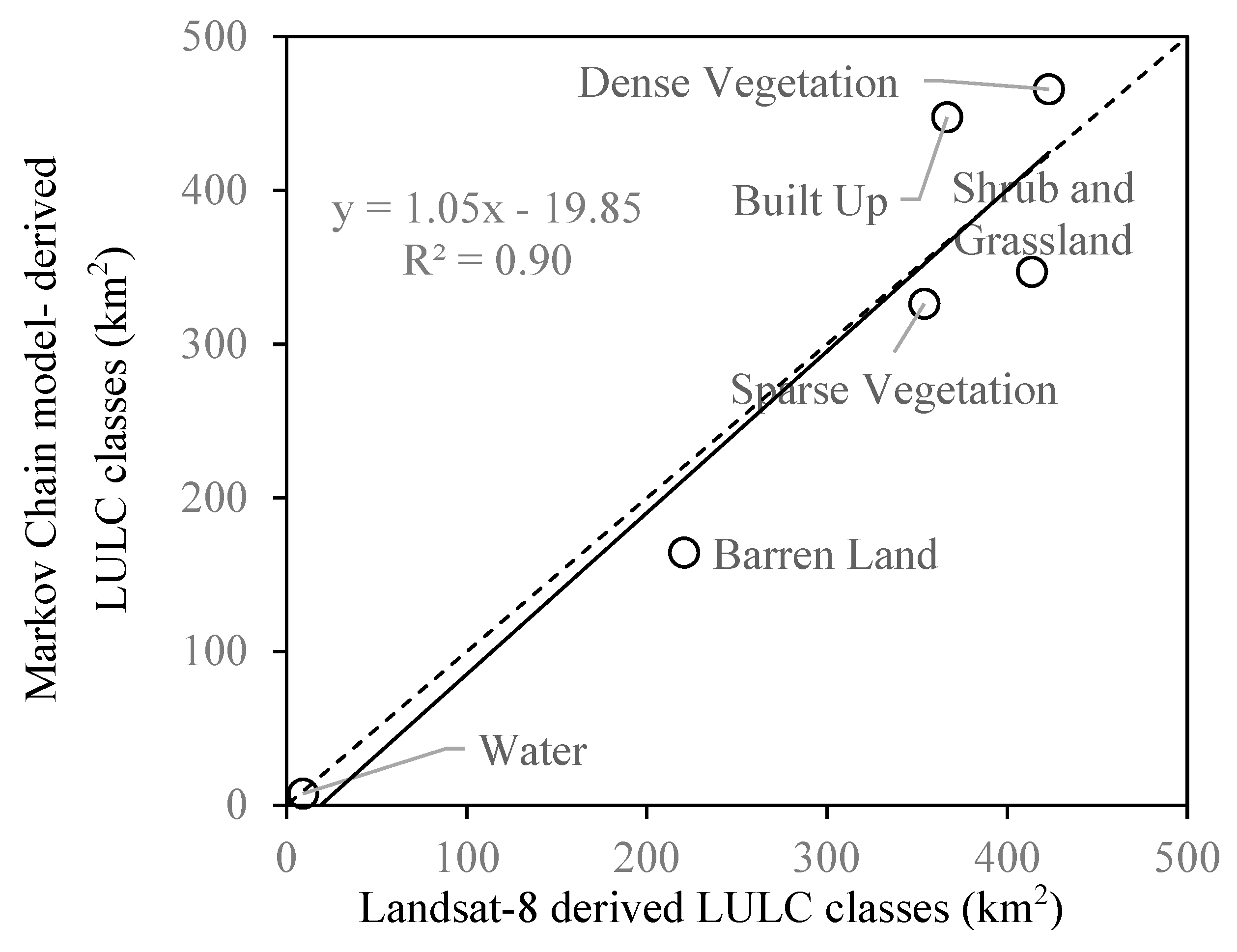
4.2. Transformation Analysis and Future Prediction of LULC Changes

The LULC transformation matrix, prepared for the period 1988–2001, is given in Table 4. From this table, it is obvious that the dominant transformation was found in built-up areas. It was noticed that the area transformed into built-up was: (i) 61.93 km2 from shrub and grassland; (ii) 57.34 km2 from barren land; (iii) 18.49 km2 from sparse vegetation; and (iv) 8.71 km2 from dense vegetation. The other noticeable transformation was for sparse vegetation. The area transformed into sparse vegetation was: (i) 126.72 km2 from shrub and grassland; and (ii) 95.40 km2 from barren land. The area transformed into dense vegetation was: (i) 114.22 km2 from barren land; (ii) 150.17 km2 from shrub and grassland; and (iii) 119.18 km2 from sparse vegetation. This transformation matrix was considered a primary matrix for future prediction of LULC in 2014, 2027, and 2040.
The transformation speed of conversion from one state to other state is required for future states. For this purpose, the LULC transformation probability matrix was derived from the LULC transformation matrix using a Markov Model, as given in Table 5. This matrix provides the transformation probability of six classes. It is unusual that the built-up areas are converted to other classes. Consequently, we assumed that its probability of changes to other classes are ‘zero’ [17]. Table 5 provides the primary transformation probability of six LULC classes during 1988–2001.
Table 6 indicates LULC classes for 1988 and 2001 derived from the Landsat-5 satellite data. On the basis of this data, a Markov model was applied to obtain LULC classes for 2014, 2027, and 2040, as given in Table 6. There is a decreasing trending of water, with 25.37 km2 in 1988 and 5.32 km2 in 2040. There is strong increasing tendency of built-up areas. The built-up area was 168.29 km2 in 1988, and it could increase to 532.74 km2 in 2027 and 625.16 km2 in 2040. The decreasing trend in barren land was noticed. It was 514.13 km2 in 1988 and it could decrease to 149.61 km2 in 2027 km2 and 137.53 km2 in 2040. Similarly, a decreasing pattern was also found in shrub and grassland, for which the area was 539.46 km2 in 1988 and it showed a reduction to 322.36 km2 in 2027 and 297.68 km2 in 2040. The sparse vegetation exhibited a decreasing trend from 319.96 km2 in 1988 to 283.37 km2 in 2040. The trend of dense vegetation showed an increasing tendency from 191.51 km2 in 1988 to 470.27 km2 in 2014, and it could decrease to 441.77 km2 in 2027 and 409.65 km2 in 2040.
Figure 3 indicates the correlation between LULC classes derived from Landsat-8 and a Markov model for 2016. The results indicated a strong relationship between them, with co-efficient of determination (R2) as 0.90. High accuracy assessment results for the year 2016 demonstrated that the classification technique used for the study area is sufficiently precise and applicable for the images from other years and study areas with similar characteristics.

5. Discussion

5.1. Accuracy of LULC Maps

We used an NDVI-based classification technique for generating LULC maps, due to its simplicity in applicability, authenticity in accuracy, and usage in recent studies [30,31,32,33]. The Landsat-8 OLI 2016 image was used to develop an LULC map by specifying NDVI values for six LULC classes on the basis of Google Earth images of 2016. The methodology, adopted for 2016, was applied to produce LULC maps for 1988 and 2001. The confusion matrices were produced for 1988 and 2001, using Kappa Statistics on the basis of 1800 sample points for each of these years, as given in Table 2 and Table 3, respectively. The overall accuracy was 90.27% and 95.11% for 1988 and 2001, respectively. This accuracy was better as compared to the accuracies of NDVI-based output maps produced in other studies; it was 81.74%, 83.91%, and 83.91% for different band combinations in a study accomplished by [30]; it was 87%, 91%, and 88% for different years in a study completed by [31]; and it was 86.15%, and 89.31% for different sub-regions in a study performed by [34]. The user and producer accuracies for individual classes were from 83.33% to 100% in both years. The accuracies for other advanced techniques used for producing maps were 80–85% [1], 78.47% [2], and 83.5% [3]. In addition, it would be worthwhile to mention that our observed overall accuracy (i.e., in the range 90.27 to 95.11%) was similar in comparison to other sophisticated approaches like KNN, SVM, and RF, as reported in Thanh Noi and Kappas [15]. The higher value of R2 indicated strong correlation between LULC classes derived from Landsat-8 and a Markov model for 2016. It further strengthens the accuracy of our methodology for LULC classification.

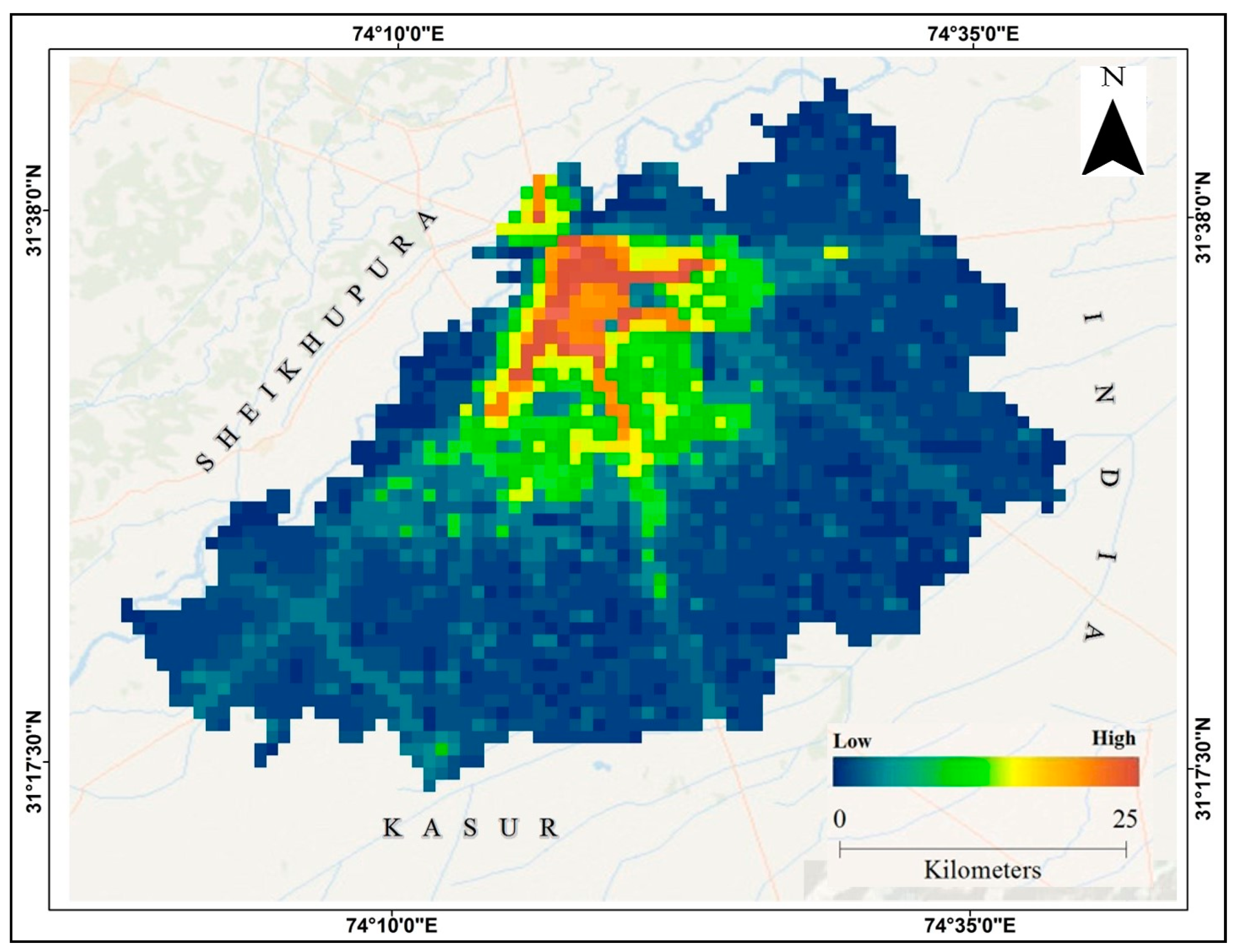
5.2. Impact of LULC Changes on Urbanization and Economy

The built-up area for District Lahore is continuously rising, and it increased by 1.89, 2.56, 3.16, and 3.71 fold, when comparing the 1988 built-up area to 2001, 2014, 2027, and 2040 respectively. A similar increasing trend of built-up area was also noticed in future forecasting for other growing cities, like Beijing in China [20]. The increasing built-up area could be related to the increasing pressure of population during different decades since 1981, as found in the case of Bangladesh [16]. According to population censuses from Pakistan Bureau of Statistics, the population of Lahore was 3.54 million in 1981, 6.34 million in 1998, and 11.12 million in 2017 [24]. The projected population could be 14.95 million in 2027 and 21.32 million in 2040, which was projected using the 2017 census population at an annual population growth rate of 3.46% [24]. To further strengthen our output of built-up sprawl with population increase, the LandScanTM data 2015 was used to plot population expansion patterns in the form of a GIS map, as given in Figure 4. LandScanTM is a global population distribution data with the finest available spatial resolution of 1 km (30” × 30”). It is developed by using best available demographic and geographic data with remote sensing imagery analysis techniques, on the basis of a multivariate dasymetric modeling framework [36]. The sprawl pattern of built-up areas, as presented in Figure 2, is comparable with the population sprawl trend obtained on the basis of LandScanTM data, as given in Figure 4. The increasing built-up trend matches with the increasing population pattern, which could be related to urbanization [7].
LULC changes affect the utilization of land for objectives that could be associated with population increase and economic growth [14]. The trend of construction of new housing societies in Lahore could be a contributing factor for increase in the built-up area with the passage of time. From Figure 4, it is obvious that the population concentration is higher in the inner part of Lahore. The population expansion trend is emerging from the inner city towards southern parts of Lahore. The construction and establishment of new societies is in this southern region. Since sufficient land was available at a reasonable cost in this area, it was utilized for construction of new luxurious residential societies, which provided comfortable and improved living standards for people. It was noticed that barren land and shrub and grassland was utilized to construct housing societies. It was observed that from 1988 to 2001, 37.42% of total barren land and grassland was transformed into built-up land. In the case of Beijing, the increasing trend for usage of cultivated land for urban built-up areas was noticed [20]. Irrigated croplands were converted into built-up areas for Hyderabad [1]. A similar transformation trend could be expected by 2040. The utilization of such land boosted the prices of residential and commercial areas and increased the real estate business in Lahore, which was also perceived in Hyderabad city in India [1]. The increase in built-up areas and agriculture was observed for the Sierra Leone city of Syria [5].
The increasing built-up area could be related to an excellent network of roads, which are multi-lane and are built to international standards. The roads are well maintained and these are expanded on the requirement of the area. Growing industries and infrastructure construction projects attracted many people from other cities and provinces around the country for better job opportunities, comfortable residence, and quality schooling. It resulted in a higher trend of migration, which eventually increased the population of Lahore. The urban migration pattern from all divisions of Pakistan to Lahore was plotted on a chord diagram, which is a graphical method for displaying the inter-relationships between migration data in a matrix. The migration data was obtained from labor force survey data for 2014–2015 through Pakistan Bureau of Statistics [24]. The results of migration patterns are presented in Figure 5. The results indicated that 35% of migrants migrated to Lahore from different districts of the Lahore division. The noticeable percentages of migration to Lahore from other divisions include: (i) 12.7% from Sahiwal; (ii) 8.9% from Faisalabad; (iii) 8.8% from Multan; (iv) 8.8% from Gujranwala; (v) 4.8% from Sargodha; (vi) 2.8% from Bahawalnagar; (vii) 2.6% from Rawalpindi; and (viii) 2.6% from Hazara Division. The percentage of migration from the rest of the divisions was from 0.2% to 1.9%.
These migration patterns show the attraction of migrants to Lahore due to better job opportunities and businesses. All these factors could have positive effects on urbanization and the economy of Lahore. Major cities in India are rapidly developing due to industrialization and rural–urban emigration [1]. The urban expansion in Hyderabad city in India had an impact on LULC and various land uses were transformed into built-up areas [1].
Lahore is Pakistan’s second largest economic hub after Karachi. It contributes 11.5% and 20.5% to the national and provincial economies, respectively. During 2010–2017, the share of Lahore increased by 1.2% points in the national economy. Its economy depends upon different sectors, which include telecommunication, information technology, manufacturing industry, engineering, pharmaceuticals, steel, chemicals, and construction material. It has planned industrial areas with an estimated 9000 industries. It is considered an important industrial city of the country and it has the largest Information Technology Park [37]. 42% of the work force is employed in the services industry, which includes finance, banking, real estate, community, cultural, and social services. It has the country’s largest software producing centers and computer industry [37].
From Table 6, it is obvious that the area for surface water could decrease to a level of 5.32 km2 from 25.37 km2 by 2040. The decrease in water area could be up to 79% during the period 1988–2040. The continuous depletion of surface water for District Lahore could be a major concern. A similar trend of decreasing water was observed for Hyderabad City in India due to increasing urban sprawl [1]. There is increasing pressure on the environment due to human displacement [5].
The surface water is mainly used for agricultural purposes in Lahore. Groundwater is extracted for drinking, domestic, industrial, and commercial purposes. Due to depletion of surface water, 10,000 tube wells were installed for agricultural purposes using groundwater. The mean annual rainfall of Lahore is 715 mm. The recharge to groundwater in the urban area is insufficient, due to built-up areas and urbanization. The groundwater discharge was higher than recharge, and it was the main factor for groundwater depletion [23]. The impact of urbanization on water resources was found to be negative. The planners and decision makers should give priority to wise usage of existing water and identifying new water resources for future generations. Another potential effect of the LULC changes is the creation of an urban heat island, due to the increase of built-up areas in particular [38].

6. Conclusions

In this study, the spatial distribution of existing and future urban land changes was investigated using remote sensing satellite data and Markov modelling for District Lahore of Pakistan. The spatial and temporal analysis was accomplished for last the twenty-eight years, during the period 1988–2016. It was revealed that there was an increase in built up, sparse, and dense vegetation, whereas there was a decrease in water, barren, and shrub and grassland. The transformations among various land cover classes were also explored during the period 1988–2001. The noticeable transformations were for dense vegetation, sparse vegetation, and built-up areas. The classes which were transformed into built-up areas were shrub and grassland, barren land, sparse vegetation, and dense vegetation. By 2040, the total percentage increase could be: (i) 271.48% for built-up; and (ii) 113.90% for dense vegetation; and the total percentage decrease could be: (i) 73.25% for barren land; (ii) 44.81% for shrub and grassland; (iii) 11.44% for sparse vegetation; and (iv) 79% for water. The commonalities in outcomes for 2016 and 2040 were constant rise in built-up areas and dense vegetation and depletion of barren land, shrub and grassland, and water. The decrease in barren land could be related to its transformation into shrub and grassland, sparse vegetation, built-up areas, and dense vegetation, as revealed in the transformation matrix.
The implication is that overall, the land cover changes and transformations were seen on a huge scale in Lahore. The different types of classes were converted mainly into built-up urban land. The entire change has greatly enhanced the standard of living for the inhabitants of Lahore, which influenced the real estate business. A large part of the barren land was utilized and converted into useful structures like housing societies, commercial buildings, and industries, which boosted industrialization and urbanization. On the other hand, this transformation likewise contributed to population increase due to relocation of individuals from the surrounding regions. Due to population increase, the pressure and threat on the available natural resources of land and water has likewise expanded.

Author Contributions

Conceptualization, T.A.A., S.I. and H.J.; methodology, T.A.A., Q.K.H. and S.I.; software, H.J. and S.I.; validation, H.J.B.; formal analysis, T.A.A., S.I., M.B. and H.J.; investigation, T.A.A., Q.K.H. and M.B.; resources, T.A.A., Q.K.H.; data Curation, T.A.A., S.I., M.B., H.J. and H.J.B.; writing—original draft preparation, T.A.A. and M.B., writing—review and editing, T.A.A. and M.B.; visualization, T.A.A., S.I., M.B., H.J.B; supervision, T.A.A.; project administration, T.A.A.; funding acquisition, Q.K.H.

Funding

This research received no external funding.

Acknowledgments

The facility and technical support provided by The Urban Unit and Advanced and Latest Informatics is acknowledged. The free access to Landsat satellite data was provided by USGS through USGS Global Visualization Viewer (GLOVIS). The use of high-resolution satellite imagery through Google Earth is also acknowledged.

Conflicts of Interest

The authors declare no conflict of interest. The funders had no role in the design of the study; in the collection, analyses, or interpretation of data; in the writing of the manuscript, or in the decision to publish the results.

References

  1. Gumma, M.K.; Mohammad, I.; Nedumaran, S.; Whitbread, A.; Lagerkvist, C.J. Urban Sprawl and Adverse Impacts on Agricultural Land: A Case Study on Hyderabad, India. Remote Sens. 2017, 9, 1136. [Google Scholar] [CrossRef]
  2. Song, J.; Lin, T.; Li, X.; Prishchepov, A.V. Mapping Urban Functional Zones by Integrating Very High Spatial Resolution Remote Sensing Imagery and Points of Interest: A Case Study of Xiamen, China. Remote Sens. 2018, 10, 1737. [Google Scholar] [CrossRef]
  3. Jia, Y.; Ge, Y.; Ling, F.; Guo, X.; Wang, J.; Wang, L.; Chen, Y.; Li, X. Urban Land Use Mapping by Combining Remote Sensing Imagery and Mobile Phone Positioning Data. Remote Sens. 2018, 10, 446. [Google Scholar] [CrossRef]
  4. Bhatta, B. Analysis of Urban Growth and Sprawl from Remote Sensing Data. Available online: https://bit.ly/2RdOeWa (accessed on 9 January 2019).
  5. Gbanie, S.P.; Griffin, A.L.; Thornton, A. Impacts on the Urban Environment: Land Cover Change Trajectories and Landscape Fragmentation in Post-War Western Area, Sierra Leone. Remote Sens. 2018, 10, 129. [Google Scholar] [CrossRef]
  6. Rimal, B.; Zhang, L.; Keshtkar, H.; Haack, B.N.; Rijal, S.; Zhang, P. Land Use/Land Cover Dynamics and Modeling of Urban Land Expansion by the Integration of Cellular Automata and Markov Chain. ISPRS Int. J. Geo-Inf. 2018, 7, 154. [Google Scholar] [CrossRef]
  7. Hegazy, I.R.; Kaloop, M.R. Monitoring urban growth and land use change detection with GIS and remote sensing techniques in Daqahlia governorate Egypt. Int. J. Sustain. Built Environ. 2015, 4, 117–124. [Google Scholar] [CrossRef] [Green Version]
  8. Yuan, F. Land-cover change and environmental impact analysis in the Greater Mankato area of Minnesota? using remote sensing and GIS modelling. Int. J. Remote Sens. 2008, 29, 1169–1184. [Google Scholar] [CrossRef]
  9. Rouse, J.W.; Haas, R.H.; Schell, J.A.; Deering, D.W. Monitoring vegetation systems in the Great Plains with ERTS. In 3rd ERTS Symposium; NASA SP-351 I; Remote Sensing Center, Texas A&M University: College Station, TX, USA, 1973; pp. 309–317. [Google Scholar]
  10. Huete, A.R. A soil-adjusted vegetation index (SAVI). Remote Sens. Environ. 1988, 25, 295–309. [Google Scholar] [CrossRef]
  11. Zha, Y.; Gao, J.; Ni, S. Use of normalized difference built-up index in automatically mapping urban areas from TM imagery. Int. J. Remote Sens. 2003, 24, 583–594. [Google Scholar] [CrossRef]
  12. Xu, H. A new index for delineating built-up land features in satellite imagery. Int. J. Remote Sens. 2008, 29, 4269–4276. [Google Scholar] [CrossRef]
  13. Xu, R.; Lin, H.; Lü, Y.; Luo, Y.; Ren, Y.; Comber, A. A Modified Change Vector Approach for Quantifying Land Cover Change. Remote Sens. 2018, 10, 1578. [Google Scholar] [CrossRef]
  14. Bonafoni, S.; Keeratikasikorn, C. Land Surface Temperature and Urban Density: Multiyear Modeling and Relationship Analysis Using MODIS and Landsat Data. Remote Sens. 2018, 10, 1471. [Google Scholar] [CrossRef]
  15. Thanh Noi, P.; Kappas, M. Comparison of Random Forest, k-Nearest Neighbor, and Support Vector Machine Classifiers for Land Cover Classification Using Sentinel-2 Imagery. Sensors 2018, 18, 18. [Google Scholar] [CrossRef] [PubMed]
  16. Hasan, S.; Deng, X.; Li, Z.; Chen, D. Projections of Future Land Use in Bangladesh under the Background of Baseline, Ecological Protection and Economic Development. Sustainability 2017, 9, 505. [Google Scholar] [CrossRef]
  17. Kumar, S.; Radhakrishnan, N.; Mathew, S. Land use change modelling using a Markov model and remote sensing. Geomatics, Natural Hazards and Risk 2013, 5, 145–156. [Google Scholar] [CrossRef] [Green Version]
  18. Pijanowski, B.; Brown, D.; Shellito, B.; Manik, G. Using neural networks and GIS to forecast land use changes: A Land Transformation Model. Comput. Environ. Urban Syst. 2002, 26, 553–575. [Google Scholar] [CrossRef]
  19. Sang, L.; Zhang, C.; Yang, J.; Zhu, D.; Yun, W. Simulation of land use spatial pattern of towns and villages based on CA–Markov model. Math. Comput. Model. 2011, 54, 938–943. [Google Scholar] [CrossRef]
  20. Han, H.; Yang, C.; Song, J. Scenario Simulation and the Prediction of Land Use and Land Cover Change in Beijing, China. Sustainability 2015, 7, 4260–4279. [Google Scholar] [CrossRef] [Green Version]
  21. Jeon, S.; Hong, H.; Kang, S. Simulation of Urban Growth and Urban Living Environment with Release of the Green Belt. Sustainability 2018, 10, 3260. [Google Scholar] [CrossRef]
  22. Maktav, D.; Erbek, F.; Jürgens, C. Remote sensing of urban areas. Int. J. Remote Sen. 2005, 26, 655–659. [Google Scholar] [CrossRef]
  23. Qureshi, A.S.; Sayed, A.H. Situation Analysis of Water Resources of Lahore: Establishing a Case for Water Stewardship Pakistan; World Wild Life Fund: Lahore, Pakistan, 2014; p. 3. [Google Scholar]
  24. Pakistan Bureau of Statistics (PBS). District wise Census Results Census 2017; 6th Population and Housing Census; Statistic House: Islamabad, Pakistan, 2017.
  25. National Aeronautics and Space Administration (NASA). Landsat 7 Science Data Users Handbook; National Aeronautics and Space Administration: Washington, DC, USA, 2011.
  26. Chander, G.; Markham, B. Revised Landsat-5 TM radiometric calibration procedures and post calibration dynamic ranges. IEEE Trans. Geosci. Remote Sens. 2003, 41, 2674–2677. [Google Scholar] [CrossRef]
  27. National Aeronautics and Space Administration (NASA). Landsat 8 Science Data Users Handbook; National Aeronautics and Space Administration: Washington, DC, USA, 2016. [Google Scholar]
  28. Shirazi, S.A.; Kazmi, S.J.H. Analysis of Population Growth and Urban Development in Lahore-Pakistan using Geospatial Techniques: Suggesting. South Asian Stud. 2014, 29, 269–280. [Google Scholar]
  29. Remote Sensing Phenology NDVI the Foundation. Available online: https://phenology.cr.usgs.gov/ndvi_foundation.php (accessed on 11 December 2018).
  30. Tang, K.; Zhu, W.; Zhan, P.; Ding, S. An Identification Method for Spring Maize in Northeast China Based on Spectral and Phenological Features. Remote Sens. 2018, 10, 193. [Google Scholar] [CrossRef]
  31. Pun, M.; Mutiibwa, D.; Li, R. Land Use Classification: A Surface Energy Balance and Vegetation Index Application to Map and Monitor Irrigated Lands. Remote Sens. 2017, 9, 1256. [Google Scholar] [CrossRef]
  32. Kong, F.; Li, X.; Wang, H.; Xie, D.; Li, X.; Bai, Y. Land Cover Classification Based on Fused Data from GF-1 and MODIS NDVI Time Series. Remote Sens. 2016, 8, 741. [Google Scholar] [CrossRef]
  33. Qiao, H.; Wu, M.; Shakir, M.; Wang, L.; Kang, J.; Niu, Z. Classification of Small-Scale Eucalyptus Plantations Based on NDVI Time Series Obtained from Multiple High-Resolution Datasets. Remote Sens. 2016, 8, 117. [Google Scholar] [CrossRef]
  34. Dadhich, P.N.; Hanaoka, S. Remote sensing, GIS and Markov’s method for land use change detection and prediction of Jaipur district. J. Geomat. 2010, 4, 9–15. [Google Scholar]
  35. Jianping, L.I.; Bai, Z.; Feng, G. RS and GIS-supported forecast of grassland degradation in southwest Songnen plain by Markov model. Geo-Spat. Inf. Sci. 2005, 8, 104–106. [Google Scholar] [CrossRef]
  36. Bhaduri, B.; Bright, E.; Coleman, P.; Urban, M.L. LandScan USA: A high-resolution geospatial and temporal modeling approach for population distribution and dynamics. GeoJournal 2007, 69, 103–117. [Google Scholar] [CrossRef]
  37. Economy of Lahore. Available online: https://en.wikipedia.org/wiki/Economy_of_Lahore (accessed on 11 December 2018).
  38. Zhou, D.; Xiao, J.; Bonafoni, S.; Berger, C.; Deilami, K.; Zhou, Y.; Frolking, S.; Yao, R.; Qiao, Z.; Sobrino, J.A. Satellite Remote Sensing of Surface Urban Heat Islands: Progress, Challenges, and Perspectives. Remote Sens. 2019, 11, 48. [Google Scholar] [CrossRef]
Figure 1. Location of the study area.
Remotesensing 11 00105 g001
Figure 2. Land cover maps for year: (a) 1988; (b) 2001; and (c) 2016.
Remotesensing 11 00105 g002
Figure 3. Comparison of the acreages of the LULC classes derived from Landsat-8 satellite data and modelling using a Markov model, during the year 2016. Model-values are obtained by linear interpolations of the projected-values between 2014 and 2027, as described in Table 6. The dash and solid lines represent 1:1 and regression lines, respectively.
Remotesensing 11 00105 g003
Figure 4. Population sprawl pattern for District Lahore using LandScanTM data.
Remotesensing 11 00105 g004
Figure 5. Chord diagram showing migration trends toward Lahore from all over Pakistan. It was prepared using Labor Force Survey 2014–2015 data obtained from Pakistan Bureau of Statistics.
Remotesensing 11 00105 g005
Table 1. Suitable normalized difference vegetation index (NDVI) ranges identified for the land cover classes.
ClassNDVI Range
Water−0.28–0.015
Built-up0.015–0.14
Barren Land0.14–0.18
Shrub and Grassland0.18–0.27
Sparse Vegetation0.27–0.36
Dense Vegetation0.36–0.74
Table 2. Accuracy assessment of land use and land cover (LULC) classification for 1988.
Landsat LULC ClassesTotal CountUser’s Accuracy
Water BodiesBuilt-upBarren LandShrub and GrasslandSparse VegetationDense Vegetation
Classified LULC ClassesWater Bodies28000000280100%
Built-up92693800031685.12%
Barren Land131260110130486%
Shrub and Grassland100028920232190.03%
Sparse Vegetation00002502027092.59%
Dense Vegetation00203027730989.64%
Total Count3003003003003003001800100%
Producer’s Accuracy93.33%90%87%96%83.33%92.33%
Total Correct: 1625 Total Samples: 1800 Overall Accuracy: 90.27% Kappa Statistics: 0.88.
Table 3. Accuracy assessment of land use and land cover (LULC) classification for 2001.
Landsat LULC ClassesTotal CountUser’s Accuracy
Water BodiesBuilt-upBarren LandShrub and GrasslandSparse VegetationDense Vegetation
Classified LULC ClassesWater Bodies29200000292100%
Built-up12751000028696.15%
Barren Land72428250332188%
Shrub and Grassland01128910530694.44%
Sparse Vegetation0046284229695.94%
Dense Vegetation0030629029996.98%
Total Count3003003003003003001800100%
Producer’s Accuracy97.3%92%94%96%94.66%96.66%
Total Correct: 1712 Total Samples: 1800 Overall Accuracy: 95.11% Kappa Statistics: 0.94.
Table 4. LULC transformation matrix during the period 1988–2001 (km2).
19882001
WaterBuilt-upBarren LandShrub and GrasslandSparse VegetationDense Vegetation
Water4.263.986.795.482.342.53
Built-up5.38102.1921.8119.7110.918.27
Barren Land6.3757.34105.09135.7195.40114.22
Shrub and Grassland2.2561.9357.72140.67126.72150.17
Sparse Vegetation0.3718.4927.2074.5280.19119.18
Dense Vegetation0.338.7119.4344.0044.4774.57
Table 5. LULC transformation probability matrix derived from the LULC transformation matrix presented in Table 4.
WaterBuilt-UpBarren LandShrub and GrasslandSparse VegetationDense Vegetation
Water0.1680.1570.2680.2160.0920.100
Built-up0.0001.0000.0000.0000.0000.000
Barren Land0.0120.1120.2040.2640.1860.222
Shrub and Grassland0.0040.1150.1070.2610.2350.278
Sparse Vegetation0.0010.0580.0850.2330.2510.372
Dense Vegetation0.0020.0450.1010.2300.2320.389
Table 6. Projected LULC acreages (km2) during the period 1988–2040. The first two rows show the dynamics as derived from the Landsat-5 satellite data.
WaterBuilt-upBarren LandShrub and GrasslandSparse VegetationDense Vegetation
198825.37168.29514.13539.46319.96191.51
200113.58318.74216.22400.38349.12460.67
20147.82432.07167.08351.57329.90470.27
20276.04532.74149.61322.36306.19441.77
20405.32625.16137.53297.68283.37409.65

