Article

Fire on the Water Towers: Mapping Burn Scars on Mount Kenya Using Satellite Data to Reconstruct Recent Fire History

Department of Geography, Miami University, Oxford, OH 45056, USA
*
Author to whom correspondence should be addressed.
Remote Sens. 2019, 11(2), 104; https://doi.org/10.3390/rs11020104
Submission received: 20 November 2018 / Revised: 31 December 2018 / Accepted: 4 January 2019 / Published: 9 January 2019
(This article belongs to the Special Issue Remote Sensing of Wildfire)

Abstract

:
Mount Kenya is one of Kenya’s ‘water towers’, the headwaters for the country’s major rivers including the Tana River and Ewaso Nyiro River, which provide water and hydroelectric power to the semiarid region. Fires affect water downstream, but are difficult to monitor given limited resources of local land management agencies. Satellite-based remote sensing has the potential to provide long term coverage of large remote areas on Mount Kenya, especially using the free Landsat data archive and moderate resolution imaging spectroradiometer (MODIS) fire products. In this study, we mapped burn scars on Mount Kenya using 30 m Landsat 7 Enhanced Thematic Mapper Plus (ETM+) and Landsat 8 Operational Land Imager (OLI) derived dNBR (change in normalized burn ratio) and MODIS active fire detection and burned area data for fires occurring from 2004 to 2015. We also analyzed topographic position (elevation, slope, aspect) of these fires using an ASTER global digital elevation model (GDEM v2) satellite-derived 30 m digital elevation model (DEM). Results indicate that dNBR images calculated from data acquired about one year apart were able to identify large fires on Mount Kenya that match locations (and timing) of MODIS active fire points and burned areas from the same time period, but we were unable to detect smaller and/or older fires.

1. Introduction

Kenya is 81.2% semiarid, arid, or very arid [1], so water is scarce, but must support subsistence agriculture, cash crops, hydroelectric power, industry, and provide water for the country’s 42 million people [2]. High elevation areas of the country provide much of the country’s water through orographic precipitation and runoff into major rivers, with Mount Kenya providing about 40% of Kenya’s water [3]. Any disruption in precipitation or runoff can have devastating consequences in this region. Land use/land cover (LULC) change and fire are the two main factors that alter mountain hydrology in Kenya [4]. In this study, we focused on the latter.
The majority of fires on Mount Kenya are human caused and this pattern has held for thousands of years [5]. Some fires are accidental, while others are set intentionally as part of agriculture, charcoal production, and poaching activities. Resources for land management agencies like Kenya Wildlife Service (KWS) and Kenya Forest Service (KFS) are extremely limited, so fires generally burn without being suppressed or extinguished. Reports on past fires are also limited and the agencies generally do not have spatially explicit data on fires. Remote sensing is a potentially valuable tool to reconstruct fire history, monitor current fires, and allow land managers to target specific areas. In this study, we tested the application of burn scar mapping methods used in other regions to see if they are feasible and can reconstruct fire history. Our objective was to test the applicability of Landsat-derived differenced normalized burn ratio (dNBR) to tropical montane forest using MODIS active fire detection and burned areas as reference due to the absence of field data. Additionally, we compared dNBR burned areas to MODIS burned area data to determine which data source is more reliable in this setting.
Burn scars refer to burned material deposited after fires, and consist mainly of ash and black carbon [6]. Immediate deposition of ash and charred material following fire provides an opportunity to map burn scars using satellite data [7]. Fire scars generally contrast strongly with unburned surfaces in the visible (0.4–0.7 μm), near infrared (0.7–1.5 μm), and middle infrared (1.5–4.0 μm) regions of the electromagnetic spectrum [7]. Fire scar mapping studies have utilized multitemporal or single post-fire data, acquired by various sensors, to successfully map burned areas and fire severity, as well as to monitor vegetation recovery after fire [8,9,10,11,12]. Fire scar mapping using optical remotely sensed data exploits the differences in the spectral signatures between healthy vegetation and vegetation that has been damaged by fire. Healthy green vegetation typically absorbs light in the red (0.6–0.7μm) wavelengths due to the presence of chlorophyll, reflects light in the near infrared (0.7–1.3 μm) through intercellular scattering, and absorbs radiation in the short-wave infrared (SWIR) (1.4–1.8 μm) due to the presence of moisture in leaf mesophyll cells [13]. Burn mapping studies have shown that more soil is exposed and vegetation partially or completely destroyed following a fire and this generally results in higher red reflectances, lower NIR reflectances, and higher SWIR reflectances [7,11]. The addition of charcoal (black and gray char) to the soil surface can however, temporarily lower the red signal [11,13]. In the single post-fire approach, the methods for burned area mapping rely on the differences in the spectral response of objects in the same image, whereas in a multitemporal approach, pre- and post-fire images are used and burned area mapping relies on differences in the spectral response of the same objects between the images [14]. Multitemporal satellite data are more advantageous than single post-fire satellite data because multitemporal data reduce the likelihood of confusion with permanent land cover types [9]. Single post-fire methods are, however, preferred to multitemporal ones because of their lower cost of data acquisition (in some cases) and effort expended in registering and processing the multitemporal data set.
Normalized burn ratio (NBR) has been used widely [15,16], as has ∆NBR or dNBR [17,18,19,20], but [21] determined that other approaches are comparable in accuracy to NBR in Mediterranean ecosystems. Multi-date analysis of both pre- and post-fire image data is often not feasible since cloud cover is a frequent problem in tropical regions. However, if most fires can be detected using once yearly image data, this potential problem may be avoided.
The normalized burn ratio (NBR) is a variation of the normalized difference vegetation index (NDVI) that incorporates near infrared (0.77–090 μm) and shortwave infrared (2.09–2.35 μm) reflectance
N B R = N I R S W I R N I R + S W I R
The dNBR is calculated from one pre- and one post-fire image
d N B R = N B R p r e f i r e N B R p o s t f i r e
Due to a wide range of land cover types in the study area that include bare volcanic rock and soils, we opted to use dNBR as single date NBR might confuse these land covers with burn scars [22,23].
In addition to mapping burn perimeters, it is important to assess burn severity (a metric largely based on loss of organic matter in the soil and above ground organic matter conversion to ash) as this has significant impact on vegetation structure, eco-hydrological processes, and social systems [24,25,26]. The most widely used field-based index for quantifying burn severity is the composite burn index (CBI), proposed by [27]. CBI field measurements are usually coupled with remotely sensed images such as Landsat TM/ETM+ data in order to map burn severity over large areas [28,29] quantified the relationships between satellite-derived surrogates of burn severity (defined using Landsat spectral indices such as dNBR) and fire intensity based on both MODIS FRP pixel and per-fire extents for 16 fires occurring across four broad vegetation types in western United States. They found that 69% of the variation in dNBR were explained by the 90th percentile of MODIS FRP, and concluded that MODIS FRP data could be used to predict potential long-term negative ecological effects for individual fires.
Much work has focused on using remote sensing to map burn scars in Africa’s savanna ecosystems [30,31], but little research has been conducted on fire mapping techniques on the East African montane ecosystems studied here [32]. Many tropical environments have a heterogeneous mix of vegetation types that vary along a topographic gradient. In the Mount Kenya area, the lower elevations are dominated by lower montane tropical forests that grade into bamboo vegetation, upper montane forests, Ericaceous vegetation to alpine vegetation at higher elevations. It is therefore not clear whether one burn scar mapping approach will be sufficient across vegetation types- especially in terms of accurately distinguishing burn severity levels.
The overall goal of this research was to map burn history using Landsat-derived differenced normalized burn ratio (dNBR) in a tropical montane environment using MODIS active fire detection and burned areas as reference data. The specific objectives of this research were to: (1) describe spatio-temporal patterns of forest fires on Mount Kenya for the period 2004–2015 using 30 m Landsat ETM+/OLI data, 500 m MODIS burned areas, and 1 km MODIS active fire product; (2) examine relationships between observed spatial patterns of fire and topographic and seasonal factors; and (3) analyze the relationship between Landsat-derived dNBR and MODIS-derived fire radiative power.

2. Materials and Methods

2.1. Study Area

Mount Kenya (Figure 1) is volcanic in origin with a climate defined by a bimodal precipitation pattern caused by shifting of the Intertropical Convergence Zone (ITCZ), and temperature patterns that are shaped more by time of day and elevation than season [33,34]. The windward side of the mountain (southeastern slopes) receives approximately 2250 mm of rainfall while the leeward side of the mountain (northwestern slopes) receives about 900 mm [35,36]. Mount Kenya is protected and under the management of the KWS and KFS. The lower fringes of the mountain are surrounded by dense settlements that engage in smallholder agriculture and have a history of encroaching on the forest areas [37].
The lower montane forests on Mount Kenya begin at elevations of 1200 m where agricultural settlements border protected areas, and extend up the mountain to elevations of 2500 m. The lower montane forests are similar in structure and general appearance to tropical rainforests in the Congo Basin [38]. Above the lower montane forests is the bamboo zone (Arundinaria alpina) at elevations of 2200–3200 m. Unlike other East African mountains, the bamboo zone on Mount Kenya is well-developed, and less fragmented. At elevations of 2500–3500 m lies the upper montane forests. These forests are smaller in stature, compared to the lower montane forests, are more open with dense grass, and are dominated by the African pencil cedar (Juniperus procera). The Ericaceous zone occurs above the tree line at elevations over 3500 m. This zone is most continuous on the eastern slope. The Paramo (also referred to as alpine zone) begins at approximately 4000 m and is characterized by dwarf vegetation. Further up from the Paramo is the Nival zone which is a cold desert belt consisting of mostly moraine, gravel, and stones [38]. Mount Kenya was inscribed as a UNESCO World Heritage Site in 1997 [39].

2.2. A History of Forest Loss, Encroachment, and Fire

A public outcry on the destruction of montane forests in Mount Kenya led to the first systematic aerial assessment of the status of Mount Kenya forests in 1999. The Mount Kenya aerial forest survey conducted between February and June 1999 revealed that the entire mountain had been heavily impacted by illegal extraction of forest products [36]. The heaviest damage was found in the bamboo zone and lower montane forests. Forest encroachment by smallholder agriculture in the lower fringes of Mount Kenya Forest was evident, while deep inside the forests, there was cultivation of Cannabis sativa. Widespread livestock grazing and frequent fires were also reported. During the five-month aerial survey, 21 active fires were spotted on the montane forests, and fire scars were evident in the drier forest zones in the northern and western slopes of the mountain. Mount Kenya is one of only two of Kenya’s water towers on the east side of the Rift Valley (the Aberdare Range being the second), feeding rivers that supply water to more than half of the country’s population and eventually flow into the Indian Ocean. LULC changes in these mountain catchments have profound impacts on water availability and quality, as well as production of hydroelectric power, which supplies about 60% of Kenya’s total electricity [3].
Fires burn frequently on Mount Kenya and in most cases, these fires are set by humans- accidentally or intentionally. Investigation of paleoecology in the region indicates that fires have occurred in the area since at least 26,000 years BP, despite the paucity of natural ignition sources [5]. Fire tolerance varies by vegetation community with grass being adapted to frequent fire, the Ericaceous zone tolerant of some fire activity, and the forests and bamboo zones lacking fire tolerance. Erica species on Mount Kenya resprout from lignotubers following fire, but require longer recovery time than grasslands. In the case of too frequent fires, grasses may invade resulting in type-conversion [40]. Over the past decade, large fires have become more common, with the following burned area totals on Mount Kenya: 3000 ha of moorland (Ericaceous zone) in 2005, 2500 ha of moorland in 2009, 3500 ha of moorland in 2009, and 3600 ha of upper montane forest in 2011 [41]. Kenyan newspaper reports indicate that over 8000 ha burned on Mount Kenya by 17 March, 2012 [42] following late arrival of “long rains”.

2.3. Data

2.3.1. Satellite Data

We obtained 12 Landsat scenes from the USGS free Landsat data archive (http://earthexplorer.usgs.gov/) for dates ranging from 2004 to 2015 (see Table 1). We used Landsat 7 ETM+ images for 2004 to 2013, then Landsat 8 OLI images for 2014 and 2015. Since local fire records [41] were only obtained for dates through 2012, we did not extend our satellite data much beyond that time (three years). Scenes for 2004 to 2012 contain missing data due to the scan line corrector failure on Landsat 7 (SLC off), but our study area is located near the scene center (Path 168, Row 60), so data gaps are minimal (<7% of pixels in our study area). Images were obtained from early in the year (all from January to March, except for one April scene) to match with the dry season that precedes the ‘long rains’ that generally begin in March. This was the best opportunity to obtain cloud-free images and also coincides with most fire activity. Any dates attributed to fires detected by Landsat are only assumed to be between each pair of near-anniversary dates images.
We obtained MODIS active fire product (hereafter referred to as MODIS fire points, or MFPs) from NASA’s Fire Information for Resource Management System (FIRMS; https://earthdata.nasa.gov/earth-observation-data/near-real-time/firms; [43]. We used the MCD14ML product (global monthly fire location product), which includes data on radiant temperature (channel 21, channel 31), fire radiative power, acquisition dates, and detection confidence [44,45]. MFPs with confidence <60% were removed before further analysis to ensure the highest likelihood of fire occurrence [19]. Confidence levels of MFPs are automatically derived as a data quality bit [45] and thus it was unnecessary to carry out an accuracy assessment.
MODIS fire points were compiled to match Landsat image dates so that all MFPs were acquired in the time that fell within the range of the pre- and post-fire Landsat images used to calculate dNBR. For example, the 2005 dNBR image was calculated from the 3 March 2004 image and 1 January 2005 images. MFPs for 4 March 2004 to 31 December 2004 were included in the analysis. Calculation of dNBR relied on availability of cloud-free Landsat images. This resulted in uneven intervals between image dates, ranging from 305 days to 432 days (Table 1). Dates of fires were determined from burn date in the MCD14ML product.
We obtained MODIS burned area product MCD64 for 2004 to 2015 from http://modis-fire.umd.edu/. We used these burned areas to compare to burn scars mapped using Landsat data (dNBR) and for fires identified by MODIS active fire detection. Dates of burn scars were determined from burn date in the MCD64 product.

2.3.2. Elevation Data

A DEM for the study area was extracted from a 30 m ASTER global digital elevation model (GDEM v2) developed jointly by the Ministry of Economy, Trade and Industry (METI) of Japan and the United States National Aeronautics and Space Administration (NASA). The GDEM was downloaded from the Land Processes Distributed Active Archive Center (LP DAAC) website managed by the NASA Earth Science Data and Information System (ESDIS) project. We calculated slope and aspect from the GDEM v2 data.

2.3.3. Fire Reports

There are no detailed field data on fires for this study area, but there are reports of some fires that include dates, location descriptions, estimated areas, and vegetation types. These KWS reports were used to corroborate MFPs and compare to Landsat mapped burned area [41].

2.4. Procedures

2.4.1. Detected Fire Characteristics

We compiled all fire points for 2004 to 2015 (May) to analyze timing of fires and topographic position. We used point locations of elevation, slope, and aspect that corresponded to center coordinates of each MODIS fire point to see if certain topographic positions burned more frequently than others. Fire points were also sorted by month to compare fire timing relative to wet and dry seasons.

2.4.2. Burn Scar Maps

Landsat 7 ETM+ and Landsat 8 OLI data were converted to at-sensor reflectance using the calibration utility in ENVI 5.0 (https://www.harrisgeospatial.com/docs/RadiometricCalibration.html) and used to calculate a normalized burn ratio image for each date. Differenced NBR (dNBR) was calculated using each pair of images (2004–2005, 2005–2006, 2006–2007, … 2014–2015) resulting in 11 dNBR images. We tested several other vegetation and burn indices (including normalized difference vegetation index, enhanced vegetation index, tasseled cap), but focused on dNBR due to poor results from other indices.
Additionally, dNBR images were rescaled to match published burn severity categories (see Table 2, [46]). Then MODIS active fire points were overlaid with dNBR images for 2004–2005 through 2014–2015. We made visual comparisons of MODIS fire points to mapped burned scars, then extracted dNBR data at each MFP for further analysis. We also made visual comparisons between dNBR mapped burns scars and MCD64 burned areas to determine if any fires were missed with Landsat data.

2.4.3. MODIS Detected Fires vs. Landsat Burn Scars

We related MODIS active fire points to mapped burn scars at two levels: first, we determined whether MODIS fire points fell into positive dNBR values (mapped as burned); then we analyzed MODIS derived fire radiative power (FRP) compared to dNBR value. The first part of the analysis is a binary comparison—does each MODIS fire point fall within a dNBR mapped fire? This was a first test of burn scar mapping accuracy to determine how many MFPs were located in areas that we mapped as burn scars using the 500 m mean dNBR (here, we used values > 0). Similar methods were used to compare FRP to mean dNBR for areas representing one MODIS pixel (1 km; [29]). The number of MFPs located in a burned area was divided by the total number of fire points for that year to obtain a percentage.
We also conducted correlation and regression analysis to explore relationships between dNBR and MODIS fire radiative power (FRP). While fire intensity and burn severity are not necessarily directly linked, we used the MFPs as a check on burn scar mapping and FRP as an indicator of fire intensity. Because we do not have details (spatial extent, severity, etc.) for all fires in the study area, we compared dNBR values point by point rather than using a summary or average over an individual fire event.
Additionally, we selected individual major fires (burn scars that could be delineated using the dNBR maps) for each year (for years that one or more discrete burn scar was visible) and extracted the single pixel dNBR and 500 m mean dNBR values for those points. We selected fires from Landsat dNBR images with clearly identifiable fire perimeters: 2004–2005, 2005–2006, 2008–2009, 2010–2011, 2011–2012 (three fires), 2013–2014. All statistical analysis was completed using Statgraphics Centurion XV (Adalta, Arezzo, Italy; STATPOINT TECHNOLOGIES INC., Warrenton, VA, USA).
Local pixel values (at each MODIS point location) and mean dNBR values for a 500-m radius around each MODIS fire point were extracted for 2004 through 2015 (see Table 1 for image pairs and dates). Landsat 7 ETM+ images for 2004 through 2012 contained SLC-off data gaps, so we eliminated any MFPs located in the gap portions of the images. Landsat 7 ETM+ scene centers (about 22% of the image, or ~36 km across) do not contain gaps, so were included. We chose to mask out points in the gap part of the images rather than remove individual points in data gaps since gaps do not match across all images and we needed to include data pixels in the 500-m radius surrounding each point to calculate means. This exclusion also applied to the 2013–2014 dNBR image since the 2013 image contained SLC-off gaps (2014 was Landsat 8 OLI; no points were in the gap areas for this year). For the 2014–2015 dNBR image, no points were removed since both scenes were Landsat 8 OLI (contained no data gaps).
Using MODIS burned area product and dNBR mapped burn scars, we compared individual fires to determine which were mapped by both Landsat dNBR, MODIS burned area, or both. We also compared areas for each burn scar, apparent timing obtained from each data source, time between fire occurrence and Landsat image acquisition (since older fires are harder to detect due to vegetation regrowth), and summarized which vegetation type was burned in each fire.
In addition to MODIS data, we obtained local reports on fire activity to corroborate our mapped burn scars. These reports contain general descriptions of location, size, cause, and year—often without specific dates included. We used these reports for general information on fires, but relied more heavily on MODIS data (active and burned areas) to verify that fires occurred. A report obtained from KWS (KWS, 2012) contains descriptions of major fires on Mount Kenya from 1932 to 2012, so we were able to compare our maps with these descriptions for burn scars mapped from 2004–2012, but not 2013–2015.

3. Results and Discussion

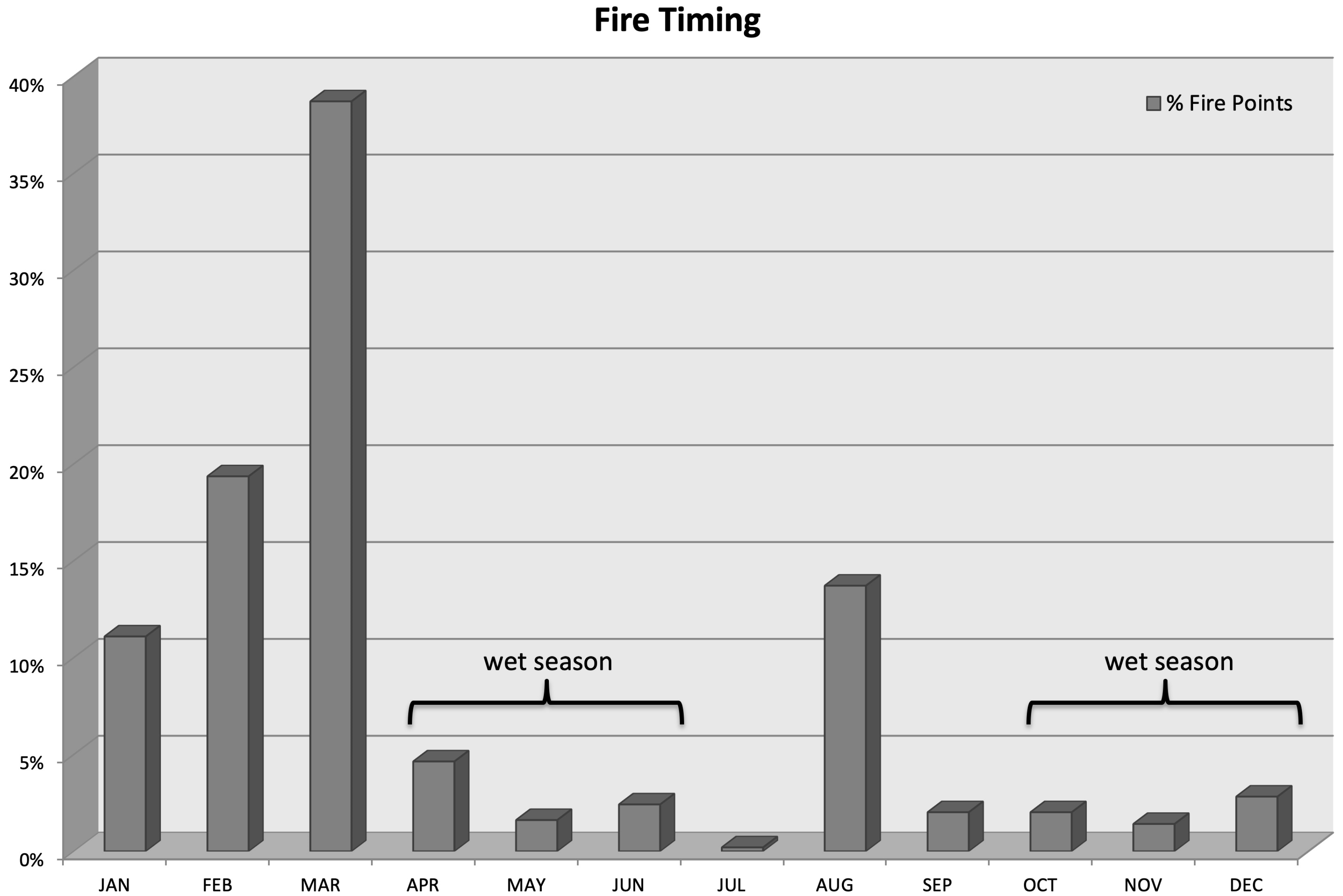
3.1. Fire Locations and Timing

We compiled MODIS fire points for 2004–2015 to check timing and topographic locations. Fire points were not evenly distributed over the year; March had the most fire points during our study period, while July had the least (see Figure 2). The timing of fires matches the bimodal precipitation patterns in Kenya, with most fires (85%) being detected in the dry seasons, especially right before the wet seasons begin. While there are two wet and two dry seasons, the short dry season (July to September (16% of MPFs) is less severe because it still has some chance of precipitation and temperatures are also cooler than the January to March dry season (69% of MFPs) [47]. Our findings mostly coincide with those of [32], although they found no fires occurring during the July-August-September dry season as we did.
The majority of fires (77%) were detected between 2500 m and 3750 m elevation (see Figure 3a), which roughly corresponds to upper montane forest and ericaceous bushland. These two vegetation types account for 81% of MODIS fire points for our study period (Figure 4, Table 3). Precipitation increases with elevation on Mount Kenya up to elevations of about 2000 m to 2500 m above which it then decreases [47]. This precipitation pattern helps explain the greater number of MODIS-detected fires above 2500 m in our study area.
Most fires were detected on lower slopes of 0° to 20° (89%), with no fires detected on slopes over 40° (Figure 3b). Detected fires were distributed across all aspects, with slightly more on northerly slopes of 270° to 90° (61%). The northern slopes of Mount Kenya are generally drier and experience many human activities including forest logging, livestock grazing, and forest fires [36]. These activities are the major threats to the continued survival of the narrow strip of forest remaining between the moorland and wheat fields to the north (Figure 1).

3.2. MODIS Active Fire Points in Mapped Burn Scars

Published fire severity ranges used with dNBR in the western United States include −0.1 to 0.1 as unburned [46], but we set 0 as the threshold for unburned in this part of the analysis since this is a new location for applying dNBR and we have no means to check the validity of the published category breakpoints at this time. Using this threshold of 0, we found that most MFPs for many of the years did fall within an area mapped as burned using Landsat-derived dNBR (see Figure 5). For the 2005–2006, 2008–2009, 2010–2011, 2011–2012, 2013–2014, and 2014–2015 dNBR images, over 80% of MODIS active fire detections were also mapped as burned areas. The remaining image pairs (2004–2005, 2006–2007, 2009–2010, and 2012–2013) had low percentage (less than 30% with most less than 20%) of MODIS active fire detection points falling within a mapped burned area. All of the image pairs with higher matches between MFP and dNBR also had visible fire perimeters that were used in further analysis except 2014–2015.
Patterns were very similar when comparing single pixel dNBR for each MFP, with the same years showing high rates of matching, although some had lower rates of matching based on single pixel dNBR. Some years with low rates of matching had better rates using single pixel dNBR: 2006–2007 and 2007–2008. Mismatches between MODIS fire detection and Landsat burns scars may be attributed to variations in severity and time since fire. Low severity fires may be missed by dNBR if the post-fire image was acquired many months later, especially if it was low severity and vegetation recovered in the meantime.

3.3. MODIS Active Fire Points vs. dNBR: Correlations

We compared fire radiative power (FRP) from the MODIS active fire data to single pixel dNBR at each point, as well as the 500-m radius mean dNBR around each point using correlation and regression analyses. We did not expect to find strong relationships or high explanatory power using FRP, but merely wanted to have some measure between fire intensity and mapped severity in the absence of field data.
There were no significant correlations for single pixel dNBR or 500-m radius dNBR compared to FRP when pooling data for all MFPs in the dataset (n = 340, Figure 6), so we also analyzed each year separately for both variables. Images dates with significant correlations between dNBR and FRP were 2006–2007, 2007–2008, 2008–2009, 2013–2014, and 2014–2015 (see Table 4). We calculated Pearson’s r and Spearman’s rho for all dates. There were a greater number of significant rank correlations than parametric. The 2006–2007 image had significant correlations for both single pixel dNBR and 500-m mean dNBR for both parametric and rank correlations. The 2013–2014 image also had significant correlations across the analysis except for parametric correlation using 500-m mean dNBR. The 2014–2015 image had significant correlations between FRP and single pixel dNBR, but not for 500-m mean dNBR.
In addition to analyzing FRP for all MFP, we also extracted data for individual burn scars for several years: 2004–2005, 2005–2006, 2008–2009, 2010–2011, 2011–2012 (three fires), and 2013–2014. We selected burn scars that were discrete and clearly visible in the Landsat imagery for this analysis. These MFPs are a subset (n = 100) of the full dataset discussed above (n = 340). There were fewer significant correlations using selected fires, but the combined MFPs from all eight fires had significant correlations for both 500-m mean dNBR and single pixel dNBR for both tests (Table 5). When testing individual years, only one had a significant correlation (single pixel dNBR vs. FRP): 2013–2014. This year had a small sample size (n = 13), but the correlation was higher than most at 0.6311 (p = 0.02). All correlations were positive for these MFP.

3.4. MODIS Active Fire Points vs. dNBR: Regressions

We ran simple regression for 500-m mean dNBR and single pixel dNBR using correlations above to select data (Table 6). This resulted in three image dates for single pixel dNBR (2006–2007, 2008–2009, 2013–2014) and five dates for 500-m mean dNBR: (2006–2007, 2007–2008, 2008–2009, 2013–2014, 2014–2015). The highest R2 among the regressions was between single pixel dNBR for 2013–2014 and FRP (0.632, p = 0.0004), although this was a small sample size (n = 13). This high explanatory power was unexpected as discussed above and did not hold for other image dates. While there were several significant regressions, only the 2013–2014 image had an R2 over 0.500. The 500-m mean dNBR for that image had an R2 of 0.550 (p = 0.0016). The lowest significant regression was for the 2008–2009 image single pixel dNBR (0.067, p = 0.0401). For all regressions, dNBR was positively correlated with FRP except for the 2007–2008 image 500-m mean dNBR, which was negative, as was indicated by the correlation analysis above. For each regression, we used the model that resulted in the best fit, which included linear, reciprocal of FRP, logarithmic FRP, square root of FRP, and dNBR squared. These transformations improved model fit, but since we do not plan to use them in a predictive fashion, they are not critical to our analysis other than to understand the connection between fire intensity and burn severity for these fires. The 2013–2014 image pair is the only one to use one Landsat 7 ETM+ scene and one Landsat 8 OLI scene. The anomalous results may be partly explained by bandwidth differences between the two instruments, since the OLI near infrared band is much narrower than ETM+ [48].
For the selected fires subset, we ran regressions for the whole dataset (n = 100) and the 2013–2014 image since both had significant correlations (Table 7). The 2013–2014 fire had higher R2 values for both 500-m mean dNBR and single pixel dNBR (0.321, p = 0.0433 and 0.426, p = 0.0155, respectively). FRP was positively correlated with dNBR for 2013–2014 and the full 100 points (as indicated by correlations described above).

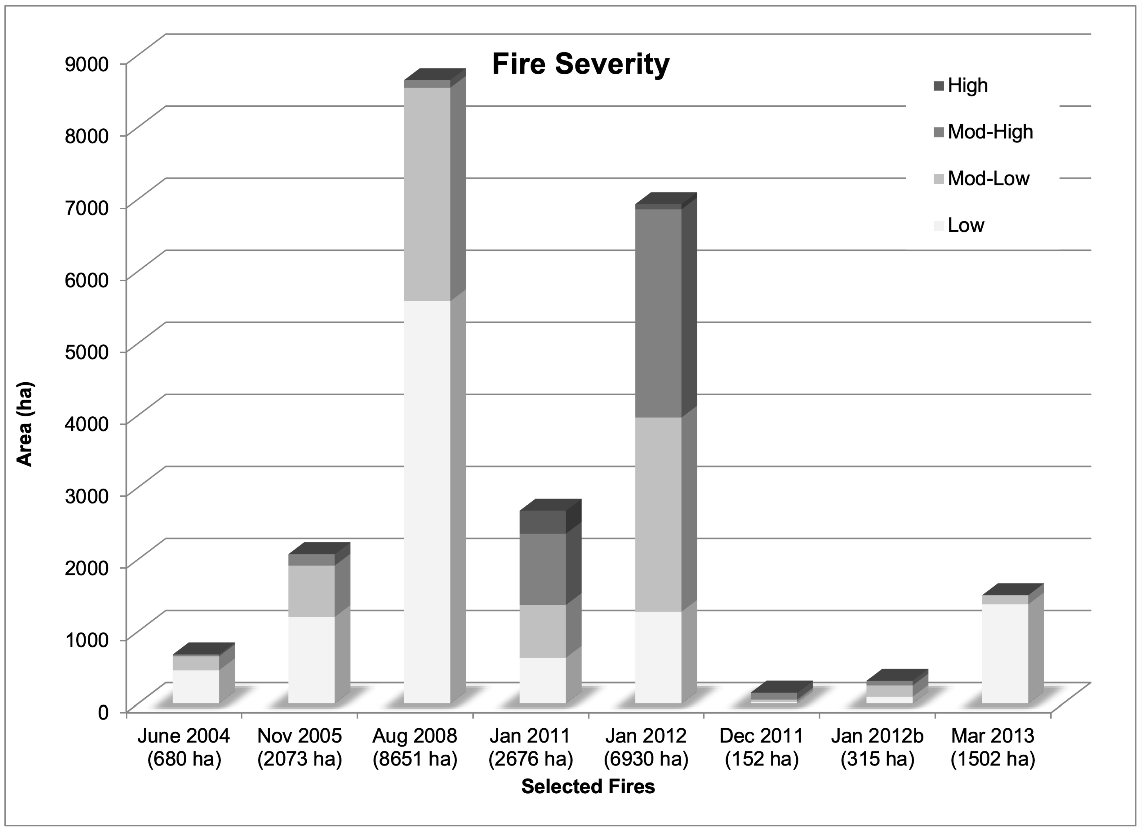
3.5. dNBR and Fire Severity

Using published dNBR ranges for fire severity (Table 2, [48]), we tabulated areas of selected fires (Figure 7, Table 8), including areas of each fire severity category for low, moderate-low, moderate-high, and high severity. It should be noted that these ranges were developed in montane conifer forests of the western United States and may not apply to these ecosystems. However, we are confident that areas mapped as burned using dNBR coincide with actual burned areas as corroborated by MODIS active fire detection, MODIS burned areas, and visual interpretation of reflectance changes. Without field data on severity, we cannot verify the severity classes, but they are a good starting point to compare dNBR ranges between fires. The minimum dNBR value for burned areas using these ranges is 0.1.
In June 2004 a fire (680 ha) burned on the east side of Mount Kenya around Lake Ellis, including areas down to about 3000 m. Another fire (2073 ha) burned on the south side of Mount Kenya in 2005 (17–18 November). The August 2008 fire was the largest mapped burned area (8651 ha), but most of the area was in the lowest dNBR range (0.1–0.27) indicating low severity fire. The January 2011 fire overlapped with part of the 2004 fire, but was larger covering 2676 ha. The larger January 2012 fire (6930 ha) burned moorland vegetation on the southwest slopes of Mount Kenya. The burned area included the same area that burned in 2005. It was recorded in newspaper accounts [42], as well as internal reporting and oblique aerial photos by Kenya Wildlife Service personnel [41]. We used a 21 January 2012 image for our post-fire image so captured the area burned up until that date. Fires were noted to have burned into February of that year [41], but no smoke is visible in the ETM+ image that we used. We identified two other fires from the 2011–2012 dNBR image: one burned in December 2011, the other also burned in January 2012, but was located on the northeast side of the mountain. Both fires were smaller (152 ha and 315 ha respectively), but showed distinctive reflectance changes between March 2011 and January 2012. A March 2013 fire burned part of the same area that burned in August 2008 on the north side of Mount Kenya.

MODIS Burned Areas vs. dNBR Burned Areas

Table 8 contains a summary of fires that were identified using MCD14ML data during the study period (3 March 2004 to 22 February 2015). The vegetation zone for each fire was determined by overlaying MCD14ML points with vegetation data. Of the 25 fires detected, most fires occurred in upper montane forest (22 of 25), while almost half were in the ericaceous zone (some fires burned in more than one vegetation type). Two fires were detected in bamboo forest, while one was detected in paramo. This pattern coincides with the distribution of combined MODIS active fire points we summarized in Figure 4.
We also calculated burned areas from MODIS burned area product (MCD64) and Landsat data (dNBR). The table also includes date of the post-fire Landsat image used to calculate dNBR with time between fire event and post-fire image date. We expected fires to become more difficult to detect using dNBR as more time passes after burning since an intervening wet season would likely cause enough vegetation regrowth to mask the burn scar. For example, the large fire that burned in early 2012 was detected using dNBR with a post-fire image acquired shortly after the January fire, but the additional area that burned in March 2012 was no longer visible in February 2013. There were no cloud-free images available for mid-2012, but from viewing previews of those partially cloud-covered Landsat scenes, it was clear that the burn scar was no longer visible by May or June of that year (following the rains of that wet season). This suggests that fire detection using dNBR is most effective if a post-fire image can be acquired shortly after the fire occurred and especially before the next wet season.
We were only able to detect burn areas using both MCD64 and dNBR for seven of the fires. Of those, some show discrepancies between the areas. MCD64 mapped two fires as patchier than the dNBR data did (August 2008 and the large January 2012 fire). In other cases, the MCD64 areas overlap but are smaller than dNBR areas (e.g., 14 January 2012). In only one case is the MCD64 area larger than the dNBR area (March 2005). The largest difference in mapped areas is the November 2005 fire, which MCD64 mapped as 200 ha, but dNBR mapped as 2073 ha. We examined the post-fire image used in the dNBR calculation (acquired 81 days after the fire) and the area appears burned. It is not clear what causes this large discrepancy.

3.6. Local Fire Reports

A report obtained from Kenya Wildlife Service [41] contains descriptions of major fires on Mount Kenya from 1932 to 2012. However, few specific dates were provided (mostly just a year) and location descriptions were difficult to reconcile with map locations. The report also contained fire sizes in hectares, but there is no description of how those areas were determined or whether they are estimates. It is also unknown whether the report is meant to serve as a complete inventory of recent fires or merely to provide examples. In most cases, the mapped fires we selected could not be matched to described fire locations in the report. Fires were listed for 2005, 2009, 2011, and 2012 (when the report was written). The fire we mapped for 2005 (17–18 November) burned in an area of moorland (and was described as “spread from northern moorland to southern moorlands”), but does not match the location name in the report. The areas are similar (mapped 2073 ha, reported as 3000 ha). We mapped no fire in 2009, but mapped a large (8651 ha) burned area on the north side of Mount Kenya in 2008 (27–30 August). For 2011, we mapped a fire 2676 ha on the east side of Mount Kenya (28–29 January) and a small fire (152 ha) near the larger fire 15 December 2011. However, location descriptions do not appear to match our mapped fire locations (place names listed are located on other parts of Mount Kenya). In 2012, the report mentions “current fire locations” that included elevation ranges near 13,000 feet (3962 m), which was suppressed by 25 January 2012. Our post-fire image was acquired 21 January 2012, but did not contain visible smoke, so we likely captured most of that fire.
Kenya Wildlife Service is most concerned with suppressing fires, but lacks resources to do so. It is unclear whether historical fire data are useful to their firefighting mission—or if fire history plays an important role in fuel loads in these ecosystems as is the case in many other regions. Since several of the burned areas we mapped burned twice during a 10-year period, this does not appear to be case, though (i.e., fuel loads do not appear to be limited by recent fires).

4. Conclusions

This research represents an early attempt to apply dNBR in a tropical montane ecosystem. Although dNBR was developed for use in forests of the western United States, the index appears potentially useful for mapping recent burned areas on Mount Kenya and can supplement field observations of local management agencies who often lack the resources to conduct detailed post-fire assessments. However, MODIS data are able to detect more fires (at a coarser resolution) so the best approach would be to start with those data.
Based on comparison of MODIS active fire detection (MCD14ML), MODIS burned area (MCD64), and Landsat dNBR, we have some recommendations for land managers in the region who wish to use remote sensing to monitor fire activity. We suggest first using MODIS active fire detection to identify likely fire locations, then follow up with MODIS burned area product (like MCD64) to refine burned areas. Once fires of interest have been identified, managers can check for availability of cloud-free Landsat imagery before and after the fire to calculate dNBR and estimate severity. It seems that the short-term visibility of burn scars limits the utility of Landsat dNBR for reconstructing fire history on Mount Kenya. These limitations will be even greater in other areas given the data gaps present in Landsat 7 ETM+ image data (Mount Kenya is located near the scene center for this path and row so was not as much of a factor for our study). Additionally, it is not clear how well Landsat 8 OLI can be used for dNBR or whether new value ranges need to be established given the significant differences in band wavelength ranges from Landsat 7 ETM+. We found that burned areas were vastly overmapped using dNBR in the years we used OLI data or a combination of ETM+ and OLI data. All of the image data used in this study are available for free, so Kenyan land managers have the option to use these methods. Given the available open source GIS and image processing software now available, managers only need a Windows-based computer and some time to process the data.
Here is a summary of our findings related to the study objectives (from Section 1):
(1) We were able to describe spatio-temporal patterns of fires on Mount Kenya for the period 2004–2015 using Landsat ETM+/OLI data, MODIS active fire product, and MODIS burned area product. This includes 81% of MFPs occurring in upper montane forest or ericaceous bushland vegetation zones. We identified burn perimeters from Landsat data for all years of the study period (2004 to 2015), but in the absence of field data, we can only estimate fire severity. It is likely that different dNBR thresholds need to be used in this region rather than those developed in the U.S. and possibly use different thresholds for each vegetation zone on Mount Kenya. Field data on fire severity would be required to develop these new thresholds.
(2) The vast majority of fires (85% of MFPs) occurred during the dry seasons (January to March; July to September), although more fires were detected in the earlier dry season (69% of MFPs) than the later one (16% of MFPs) during our study period. Fires tend to occur on more northerly slopes (61% of MPFs) between 2500 m and 3750 m elevation (77% of MFPs).
(3) We found significant relationships (p < 0.05) between fire radiative power (FRP) and dNBR for several years of the study period and for specific fires, although there is not a direct link in all cases as others have reported [49].
One issue that requires further study is incorporation of field-based severity measures shortly after fire events, using protocols similar to burned area emergency response (BAER) teams [50] in the U.S. This is currently not feasible given the limited resources of KWS and KFS, but a pilot study might be sufficient to develop dNBR thresholds more compatible with the vegetation in this region. Additionally, it would be useful to further investigate the impact of using ETM+ vs. OLI for calculating dNBR given the differences in spectral bandwidths. Our results indicate that OLI dNBR overestimated burned areas compared to ETM+, but adjusting dNBR thresholds might compensate for this problem. Finally, it would be advisable to include additional image dates through the year to capture burn scars from less severe fires. Since our Landsat images were acquired about a year apart, it is possible that we missed smaller or less severe fires, particularly if the pre-fire image was shortly before the fire and vegetation was able to recover by the post-fire image. Despite these limitations, we believe that Landsat (or similar sensors) can be used to map burn scars in this region.

Author Contributions

All authors contributed to this manuscript: Conceptualization, Methodology, M.C.H., J.K.M., and J.L.M.; Formal analysis, M.C.H.; Data curation, M.C.H.; Writing—original draft preparation, M.C.H.; Writing—review and editing, M.C.H., J.K.M., and J.L.M.

Funding

This research received no external funding.

Acknowledgments

The authors wish to thank Simon Gitau of Kenya Wildlife Service, Mount Kenya Region for sharing a report on Mount Kenya fire activity. The authors also wish to thank four anonymous reviewers for their suggestions on improving the manuscript.

Conflicts of Interest

The authors declare no conflict of interest.

References

  1. Sombroek, W.G.; Braun, H.M.H.; van der Pouw, B.J.A. Exploratory Soil Map and Agro-Climatic Zone Map of Kenya, 1980. Scale: 1:1,000,000. In Exploratory Soil Survey Report No. E1; Kenya Soil Survey Ministry of Agriculture—National Agricultural Laboratories: Nairobi, Kenya, 1982. [Google Scholar]
  2. Kenya National Bureau of Statistics. Home—Kenya National Bureau of Statistics, Nairobi, Kenya. Available online: https://www.knbs.or.ke/ (accessed on 12 August 2018).
  3. Kenya, Atlas of Our Changing Environment; United Nations Environment Programme: Nairobi, Kenya, 2009.
  4. Hemp, A. Climate change-driven forest fires marginalize the impact of ice cap wasting on Kilimanjaro. Glob. Chang. Biol. 2005, 11, 1013–1023. [Google Scholar] [CrossRef]
  5. Rucina, S.M.; Muiruri, V.M.; Kinyanjui, R.N.; McGuiness, K.; Marchant, R. Late Quaternary vegetation and fire dynamics on Mount Kenya. Palaeogeogr. Palaeoclimatol. Palaeoecol. 2009, 283, 1–14. [Google Scholar] [CrossRef]
  6. Kuhlbusch, T.; Crutzen, P. Black carbon, the global carbon cycle, and atmospheric carbon dioxide. In Biomass Burning and Global Change, Volume 1: Remote Sensing, Modeling, and Inventory Development, and Biomass Burning in Africa; The MIT Press: Cambridge, MA, USA, 1996; Volume 1, pp. 160–169. [Google Scholar]
  7. Fuller, D.O. Satellite remote sensing of biomass burning with optical and thermal sensors. Prog. Phys. Geogr. Earth Environ. 2000, 24, 543–561. [Google Scholar] [CrossRef]
  8. Chuvieco, E.; Congalton, R.G. Using Cluster Analysis to Improve the Selection of Training Statistics in Classifying Remotely Sensed Data. Photogramm. Eng. 1988, 54, 1275–1281. [Google Scholar]
  9. Pereira, J.M.C.; Chuvieco, E.; Beaudoin, A.; Desbois, N. Remote sensing methods for the study of large wildfires: A review. In Report of the Megafires Project; Universidad de Alcala: Alcala de Henares, Spain, 1997; pp. 127–183. [Google Scholar]
  10. Koutsias, N.; Karteris, M. Logistic regression modelling of multitemporal Thematic Mapper data for burned area mapping. Int. J. Remote Sens. 1998, 19, 3499–3514. [Google Scholar] [CrossRef]
  11. Rogan, J.; Yool, S.R. Mapping fire-induced vegetation depletion in the Peloncillo Mountains, Arizona and New Mexico. Int. J. Remote Sens. 2001, 22, 3101–3121. [Google Scholar] [CrossRef]
  12. Maingi, J.K. Mapping Fire Scars in a Mixed-Oak Forest in Eastern Kentucky, USA, Using Landsat ETM+ Data. Geocarto Int. 2005, 20, 51–63. [Google Scholar] [CrossRef]
  13. Gerard, F.; Plummer, S.; Wadsworth, R.; Sanfeliu, A.F.; Iliffe, L.; Balzter, H.; Wyatt, B. Forest fire scar detection in the boreal forest with multitemporal SPOT-VEGETATION data. IEEE Trans. Geosci. Remote Sens. 2003, 41, 2575–2585. [Google Scholar] [CrossRef]
  14. Koutsias, N.; Karteris, M. Burned area mapping using logistic regression modeling of a single post-fire Landsat-5 Thematic Mapper image. Int. J. Remote Sens. 2000, 21, 673–687. [Google Scholar] [CrossRef]
  15. Cocke, A.E.; Fulé, P.Z.; Crouse, J.E. Comparison of burn severity assessments using Differenced Normalized Burn Ratio and ground data. Int. J. Wildland Fire 2005, 14, 189–198. [Google Scholar] [CrossRef]
  16. Escuin, S.; Navarro, R.; Fernández, P. Fire severity assessment by using NBR (Normalized Burn Ratio) and NDVI (Normalized Difference Vegetation Index) derived from LANDSAT TM/ETM images. Int. J. Remote Sens. 2008, 29, 1053–1073. [Google Scholar] [CrossRef]
  17. van Wagtendonk, J.W.; Root, R.R.; Key, C.H. Comparison of AVIRIS and Landsat ETM+ detection capabilities for burn severity. Remote Sens. Environ. 2004, 92, 397–408. [Google Scholar] [CrossRef]
  18. Miller, J.D.; Thode, A.E. Quantifying burn severity in a heterogeneous landscape with a relative version of the delta Normalized Burn Ratio (dNBR). Remote Sens. Environ. 2007, 109, 66–80. [Google Scholar] [CrossRef]
  19. McCarty, J.L.; Loboda, T.; Trigg, S. A Hybrid Remote Sensing Approach to Quantifying Crop Residue Burning in the United States. Appl. Eng. Agric. 2008, 24, 515–527. [Google Scholar] [CrossRef]
  20. Moody, J.A.; Ebel, B.A.; Nyman, P.; Martin, D.A.; Stoof, C.; McKinley, R. Relations between soil hydraulic properties and burn severity. Int. J. Wildland Fire 2016, 25, 279–293. [Google Scholar] [CrossRef]
  21. Mallinis, G.; Koutsias, N. Comparing ten classification methods for burned area mapping in a Mediterranean environment using Landsat TM satellite data. Int. J. Remote Sens. 2012, 33, 4408–4433. [Google Scholar] [CrossRef]
  22. Bastarrika, A.; Chuvieco, E.; Martin, P. Mapping burned areas from Landsat TM/ETM+ data with a two-phase algorithm: Balancing omission and commission errors-ScienceDirect. Remote Sens. Environ. 2011, 115, 1003–1012. [Google Scholar] [CrossRef]
  23. Veraverbeke, S.; Lhermitte, S.; Verstraeten, W.W.; Goossens, R. Evaluation of pre/post-fire differenced spectral indices for assessing burn severity in a Mediterranean environment with Landsat Thematic Mapper. Int. J. Remote Sens. 2011, 32, 3521–3537. [Google Scholar] [CrossRef] [Green Version]
  24. Goetz, S.J.; Mack, M.C.; Gurney, K.R.; Randerson, J.T.; Houghton, R.A. Ecosystem responses to recent climate change and fire disturbance at northern high latitudes: Observations and model results contrasting northern Eurasia and North America. Environ. Res. Lett. 2007, 2, 045031. [Google Scholar] [CrossRef]
  25. Adams, H.D.; Luce, C.H.; Breshears, D.D.; Allen, C.D.; Weiler, M.; Hale, V.C.; Smith, A.M.; Huxman, T.E. Ecohydrological consequences of drought- and infestation-triggered tree die-off: Insights and hypotheses. Ecohydrology 2012, 5, 145–159. [Google Scholar] [CrossRef]
  26. McCool, S.F.; Burchfield, J.A.; Williams, D.R.; Carroll, M.S. An Event-Based Approach for Examining the Effects of Wildland Fire Decisions on Communities. Environ. Manag. 2006, 37, 437–450. [Google Scholar] [CrossRef] [PubMed]
  27. Key, C.H.; Benson, N.C. Landscape Assessment (LA). In Lutes, Duncan C.; Keane, Robert E.; Caratti, John F.; Key, Carl H.; Benson, Nathan C.; Sutherland, Steve; Gangi, Larry J. 2006. FIREMON: Fire Effects Monitoring and Inventory System. Gen. Tech. Rep. RMRS-GTR-164-CD. Fort Collins, CO: U.S. Department of Agriculture, Forest Service, Rocky Mountain Research Station. p. LA-1-55; U.S. Department of Agriculture: Washington, DC, USA, 2006; Volume 164. [Google Scholar]
  28. de Santis, A.; Chuvieco, E. GeoCBI: A modified version of the Composite Burn Index for the initial assessment of the short-term burn severity from remotely sensed data. Remote Sens. Environ. 2009, 113, 554–562. [Google Scholar] [CrossRef]
  29. Heward, H.; Smith, A.M.; Roy, D.P.; Tinkham, W.T.; Hoffman, C.M.; Morgan, P.; Lannom, K.O. Is burn severity related to fire intensity? Observations from landscape scale remote sensing. Int. J. Wildland Fire 2013, 22, 910–918. [Google Scholar] [CrossRef]
  30. Landmann, T. Characterizing sub-pixel Landsat ETM+ fire severity on experimental fires in the Kruger National Park, South Africa: Research letter. S. Afr. J. Sci. 2003, 99, 357–360. [Google Scholar]
  31. Hudak, A.T.; Brockett, B.H. Mapping fire scars in a southern African savannah using Landsat imagery. Int. J. Remote Sens. 2004, 25, 3231–3243. [Google Scholar] [CrossRef]
  32. Downing, T.A.; Imo, M.; Kimanzi, J. Fire occurrence on Mount Kenya and patterns of burning. GeoResJ 2017, 13, 17–26. [Google Scholar] [CrossRef]
  33. Schmitt, K. The Vegetation of the Aberdare National Park Kenya; Universitätsverlag Wagner: Innsbruck, Austria, 1991. [Google Scholar]
  34. Bussmann, R.W. The Forests of Mount Kenya (Kenya)-Vegetation, Ecology, Destruction and Management of A Tropical Mountain Forest Ecosystem; Universität Bayreuth: Bayreuth, Germany, 1994. [Google Scholar]
  35. Thompson, B.W. The Mean Annual Rainfall of Mount Kenya. Weather 1966, 21, 48–49. [Google Scholar] [CrossRef]
  36. Gathaara, G.N. Aerial Survey of the Destruction of Mt. Kenya, Imenti and Ngare Ndare Forest Reserves February-June 1999; FAO: Rome, Italy, 1999; p. 33. [Google Scholar]
  37. Notter, B.; MacMillan, L.; Viviroli, D.; Weingartner, R.; Liniger, H.-P. Impacts of environmental change on water resources in the Mt. Kenya region. J. Hydrol. 2007, 343, 266–278. [Google Scholar] [CrossRef]
  38. Niemelä, T.; Pellikka, P. Zonation and Characteristics of the Vegetation of Mt; University of Helsinki: Helsinki, Finland, 2004; p. 7. [Google Scholar]
  39. UNESCO World Heritage. Mount Kenya National Park/Natural Forest. UNESCO World Heritage Centre. Available online: https://whc.unesco.org/en/list/800/ (accessed on 12 August 2018).
  40. Wesche, K.; Miehe, G.; Kaeppeli, M. The Significance of Fire for Afroalpine Ericaceous Vegetation. Mt. Res. Dev. 2000, 20, 340–347. [Google Scholar] [CrossRef]
  41. Kenya Wildlife Service. Mount Kenya Forest Fire Overview; Kenya Wildlife Service: Nairobi, Kenya, 2012.
  42. Njagi, J. Raging fires destroy forests on Mt Kenya and Aberdares. Daily Nation, 17 March 2012. [Google Scholar]
  43. Davies, D.K.; Ilavajhala, S.; Wong, M.M.; Justice, C.O. Fire Information for Resource Management System: Archiving and Distributing MODIS Active Fire Data. IEEE Trans. Geosci. Remote Sens. 2009, 47, 72–79. [Google Scholar] [CrossRef]
  44. Justice, C.O.; Giglio, L.; Roy, D.; Boschetti, L.; Csiszar, I.; Davies, D.; Korontzi, S.; Schroeder, W.; O’Neal, K.; Morisette, J. MODIS-derived global fire products. In Land Remote Sensing and Global Environmental Change; Springer: New York, NY, USA, 2010; pp. 661–679. [Google Scholar]
  45. Giglio, L.; Descloitres, J.; Justice, C.O.; Kaufman, Y.J. An Enhanced Contextual Fire Detection Algorithm for MODIS. Remote Sens. Environ. 2003, 87, 273–282. [Google Scholar] [CrossRef]
  46. United States Geological Survey (USGS). The Normalized Burn Ratio (NBR)-Brief Outline of Processing Steps; USGS: Reston, VA, USA, 2004; p. 1.
  47. Camberlin, P.; Boyard-Micheau, J.; Philippon, N.; Baron, C.; Leclerc, C.; Mwongera, C. Climatic gradients along the windward slopes of Mount Kenya and their implication for crop risks. Part 1: Climate variability. Int. J. Climatol. 2014, 34, 2136–2152. [Google Scholar] [CrossRef]
  48. Schroeder, W.; Oliva, P.; Giglio, L.; Quayle, B.; Lorenz, E.; Morelli, F. Active fire detection using Landsat-8/OLI data. Remote Sens. Environ. 2016, 185, 210–220. [Google Scholar] [CrossRef] [Green Version]
  49. Csiszar, I.; Loboda, T.; French, N.H.F.; Giglio, L.; Hockenberry, T.L. A Multi-Sensor Approach to Fine-Scale Fire Characterization; University of Maryland: College Park, MD, USA, 2014; p. 4. [Google Scholar]
  50. USDA Forest Service. Watershed-WFW-Watershed, Fish, Wildlife, Air & Rare Plants-USDA Forest Service. Available online: https://www.fs.fed.us/biology/watershed/burnareas/background.html (accessed on 12 August 2018).
Figure 1. Location of study in Central Kenya with vegetation zones and MODIS active fire detection points shown (2004–2015). Gray rectangle on locator map shows location of Mount Kenya and inset map. All towns and cities (in red) are labeled with names, MODIS data are shown as black triangles with no labels.
Remotesensing 11 00104 g001
Figure 2. Distribution of MODIS active fire detection points by month, including rainfall timing.
Remotesensing 11 00104 g002
Figure 3. Proportion of MODIS active fire detection points by (a) elevation, (b) slope, and (c) aspect class.
Remotesensing 11 00104 g003
Figure 4. Distribution of MODIS active fire detection points by vegetation zone.
Remotesensing 11 00104 g004
Figure 5. Percentage of MODIS active fire detection points (MFP) located in mapped burned areas from Landsat ETM+ and OLI data 2004–2005 to 2014–2015.
Remotesensing 11 00104 g005
Figure 6. Fire radiative power from MODIS active fire detection compared with mean Landsat (ETM+ or OLI) dNBR for 500 m radius around each 1 km MODIS fire points, 2004–2005 to 2014–2015.
Remotesensing 11 00104 g006
Figure 7. Areas of selected visible burn scars at 30 m resolution with estimated severity measured from ETM+ and OLI dNBR.
Remotesensing 11 00104 g007
Table 1. List of Landsat images used this study.
Image DateInstrumentDays between Images
3-Mar-04ETM+--
1-Jan-05ETM+305
5-Feb-06ETM+400
8-Feb-07ETM+367
26-Jan-08ETM+352
13-Feb-09ETM+384
21-Apr-10ETM+432
7-Mar-11ETM+320
21-Jan-12ETM+320
24-Feb-13ETM+400
3-Feb-14OLI344
22-Feb-15OLI384
Table 2. Fire severity classes assigned to dNBR ranges (from [46]).
dNBRBurn Severity
<−0.25High post-fire regrowth
−0.25 to −0.1Low post-fire regrowth
−0.1 to +0.1Unburned
0.1 to 0.27Low-severity burn
0.27 to 0.44Moderate-low severity burn
0.44 to 0.66Moderate-high severity burn
>0.66High-severity burn
Table 3. Elevation ranges for each vegetation zone on Mount Kenya, from [38].
Vegetation ZoneElevation Range (m)
Nival4144–5065
Paramo3354–4760
Ericaceous Bushland2990–4245
Upper Montane Forest2651–3876
Bamboo Forest2120–3283
Lower Montane Forest1442–3116
Table 4. Correlations between dNBR and MODIS fire radiative power.
All MODIS Fire Pts
Pearson’s r
DateSingle Pixel dNBRp500 m Mean dNBRpn
2006–20070.38820.00530.37940.006650
2013–20140.56460.0283----15
2014–2015-----0.46890.020824
All MODIS Fire Pts
Spearman’s rho
DateSingle Pixel dNBRp500 m Mean dNBRpn
2006–20070.34820.01480.34570.015550
2007–2008----−0.51080.035218
2008–20090.32880.00960.25910.041463
2013–20140.68210.01070.63570.017415
2014–2015----−0.55040.008324
Table 5. Correlations between dNBR and MODIS fire radiative power for select fires.
Selected FiresSingle Pixel dNBRp500 m Mean dNBRpn
All Points0.21950.02820.31240.0016100
2013–20140.63110.0207----13
Spearman’s rho
Selected FiresSingle Pixel dNBRp500 m Mean dNBRpn
All Points0.28040.00530.30890.0021100
2013–2014----------
Table 6. Regressions between dNBR and MODIS fire radiative power.
All MODIS Fire Pts
500 m Mean dNBR
DateInterceptSlopeFRPpR2
2006–2007−0.0800510.0002520X0.00660.144
2007–20080.250982−0.0613224ln(X)0.04060.237
2008–20090.179452−2.27282001/X0.01900.869
2013–20140.242368−6.20080001/X0.00160.550
2014–20150.220174−0.0337444ln(X)0.00750.283
All MODIS Fire Pts
Single Pixel dNBR
DateInterceptSlopeFRPpR2
2006–2007−0.1127650.0007947X0.00530.151
2008–2009−0.1425670.0637314ln(X)0.04010.672
2013–20140.261226−7.3644400ln(X)0.00040.632
Table 7. Regressions between dNBR and MODIS fire radiative power for select fires.
DataInterceptSlopeFRPpR2
All500 m Mean dNBR0.122,9470.009,114,5sqrt(X)0.00110.104
AllSingle Pixel dNBR0.125,520.010,018,1sqrt(X)0.02050.536
2014500 m Mean dNBR0.031,1730.026,599,8ln(X)0.04330.321
2014Single Pixel dNBR0.008,1010.000,166,4sqrt(Y)0.01550.426
Table 8. Summary of fires detected using Landsat dNBR, MODIS active fire, and MODIS burned areas. BA = bamboo forest, EB = ericaceous bushland, UM = upper montane forest, PA = paramo. Fires marked with * are those included in Section 3.5.
Fire (MCD14ML)Vegetation ZoneArea (ha) (MCD64)Area (ha) (dNBR)Landsat Post-Fire DateDays since Fire
East Side
6/2/2004*
UM/ EBX7201/1/2005213
N-NW Side
3/9/2005
UM5252802/5/2006334
SW Side
11/17/2005–11/18/2005*
UM/ EB20020732/5/200681
East Side
2/8/2006–2/16/2006
UM/ EB/ PA10275X2/8/2007357
Bamboo
2/21/2006–2/23/2006
BAXX2/8/2007350
NE Side
3/6/2007–3/7/2007
UM/EB10275X1/26/2008325
North Side
5/20/2007–5/22/2007
UMXX1/26/2008249
NW Side
2/24/2008–2/27/2008
UM525na2/13/2009352
NW Side High Elev
3/5/2008
UM225na2/13/2009345
8/27/2008–8/30/2008*UM/EB625086512/13/2009167
Bamboo
3/3/2009, 3/26/2009
BAXX4/21/2010391
North Side
3/24/2009–3/28/2009
EB/UM5425X4/21/2010389
Near East Side
12/31/2010
UMXna3/7/201166
East Side
1/28/2011–1/29/2011*
UM/EB227526763/7/201137
North Side
3/11/2011
UM1050X1/21/2012316
NW Side
4/12/2011–4/13/2011
UM850na1/21/2012283
NE Side
12/15/2011*
UM1501601/21/201237
NE Side
1/14/2012*
UM2254401/21/20127
South Side
1/17/2012–1/19/2012*
UM/EB596769301/21/20122
North Side
2/8/2012–2/10/2012
UM1650X2/24/2013380
High Elev
3/13/2012
PA1975na2/24/2013348
SE Side
3/18/2012–3/21/2012
EB/UM150X2/24/2013340
North Side
3/1/2013–3/5/2013*
UM/EB1275na2/3/2014335
North Side
8/16/2014–8/17/2014
UM1475na2/22/2015189
North Side
9/27/2014
UM125na2/22/2015148

