Detecting Spatiotemporal Changes in Vegetation with the BFAST Model in the Qilian Mountain Region during 2000–2017


Abstract
1. Introduction
2. Materials and Methods
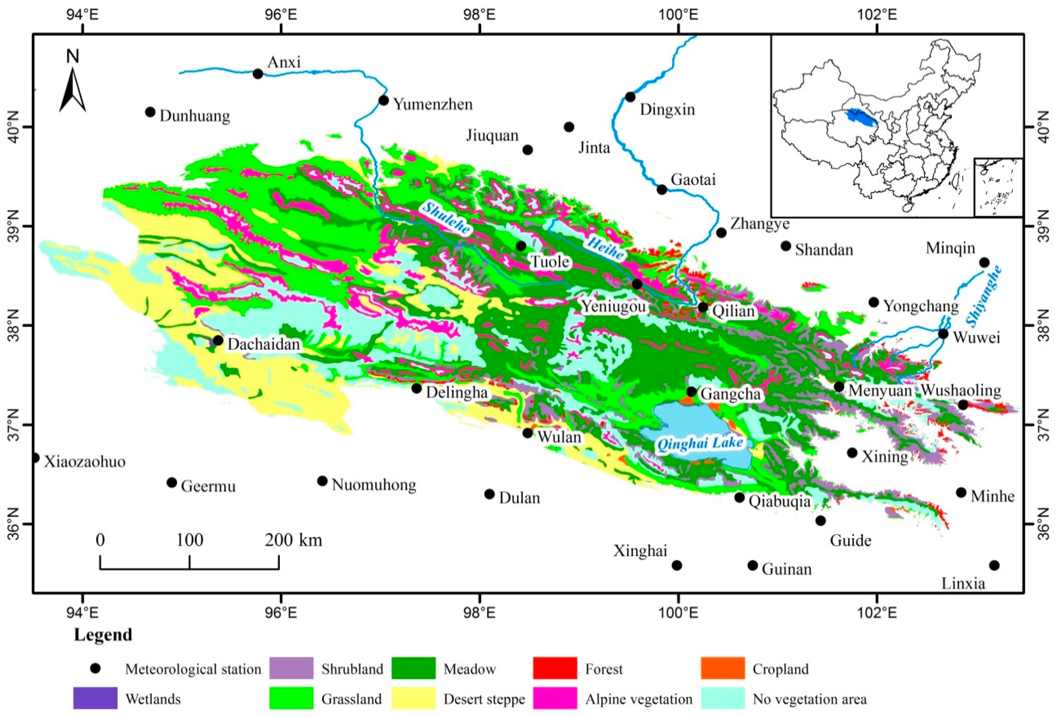
2.1. Study Area
2.2. Datasets
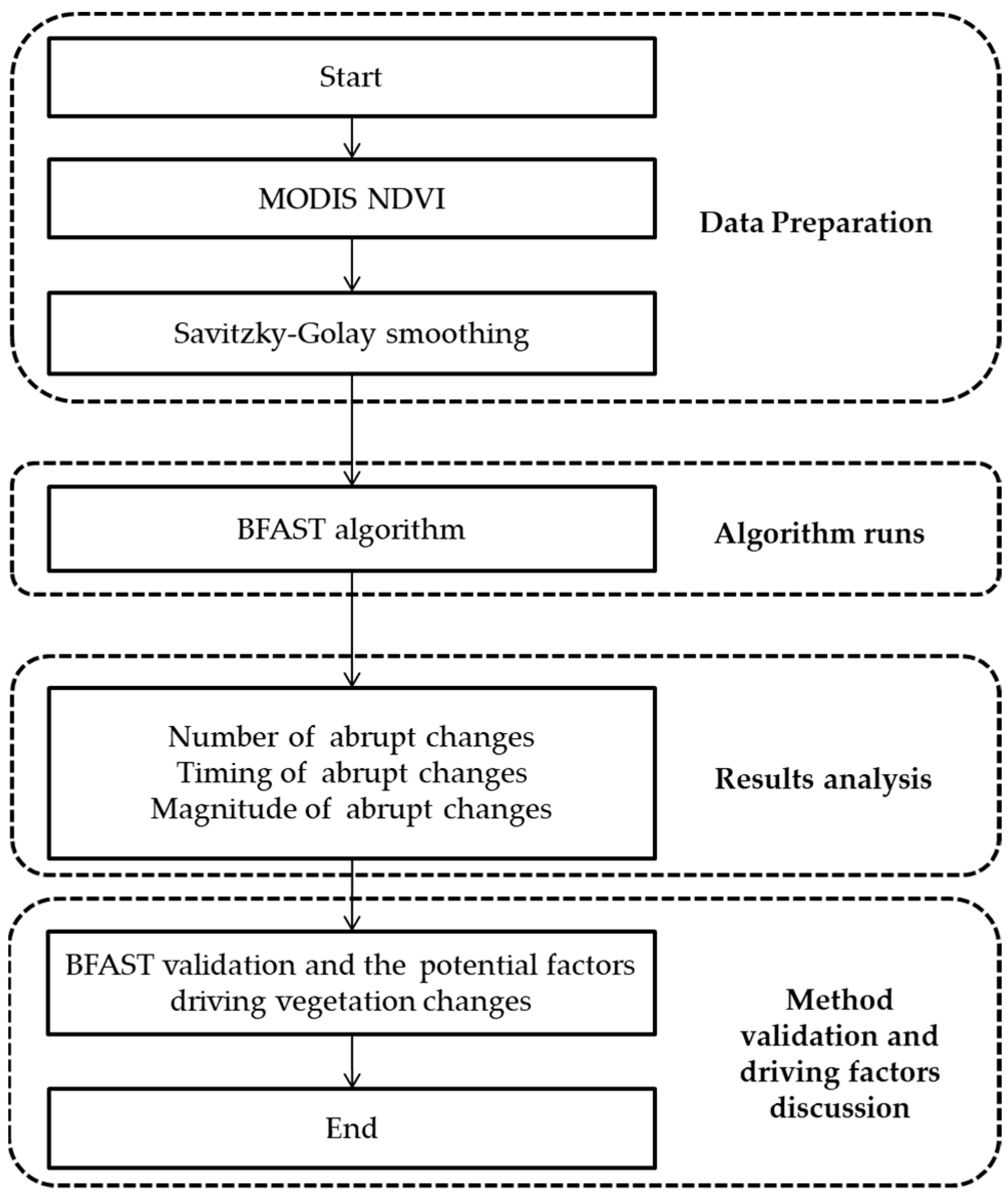
3. Methodologies
3.1. Preparation of High-Quality NDVI Datasets
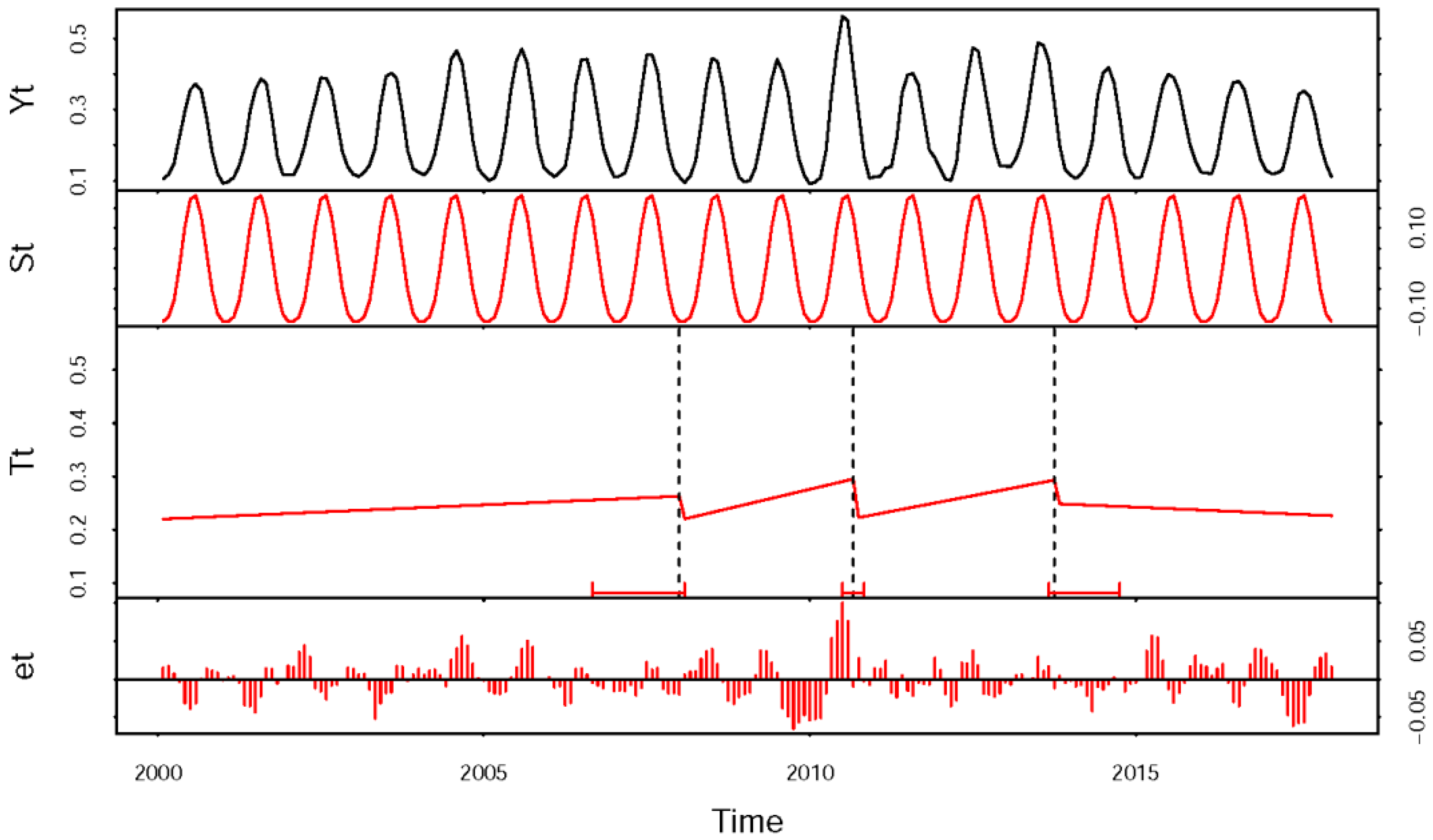
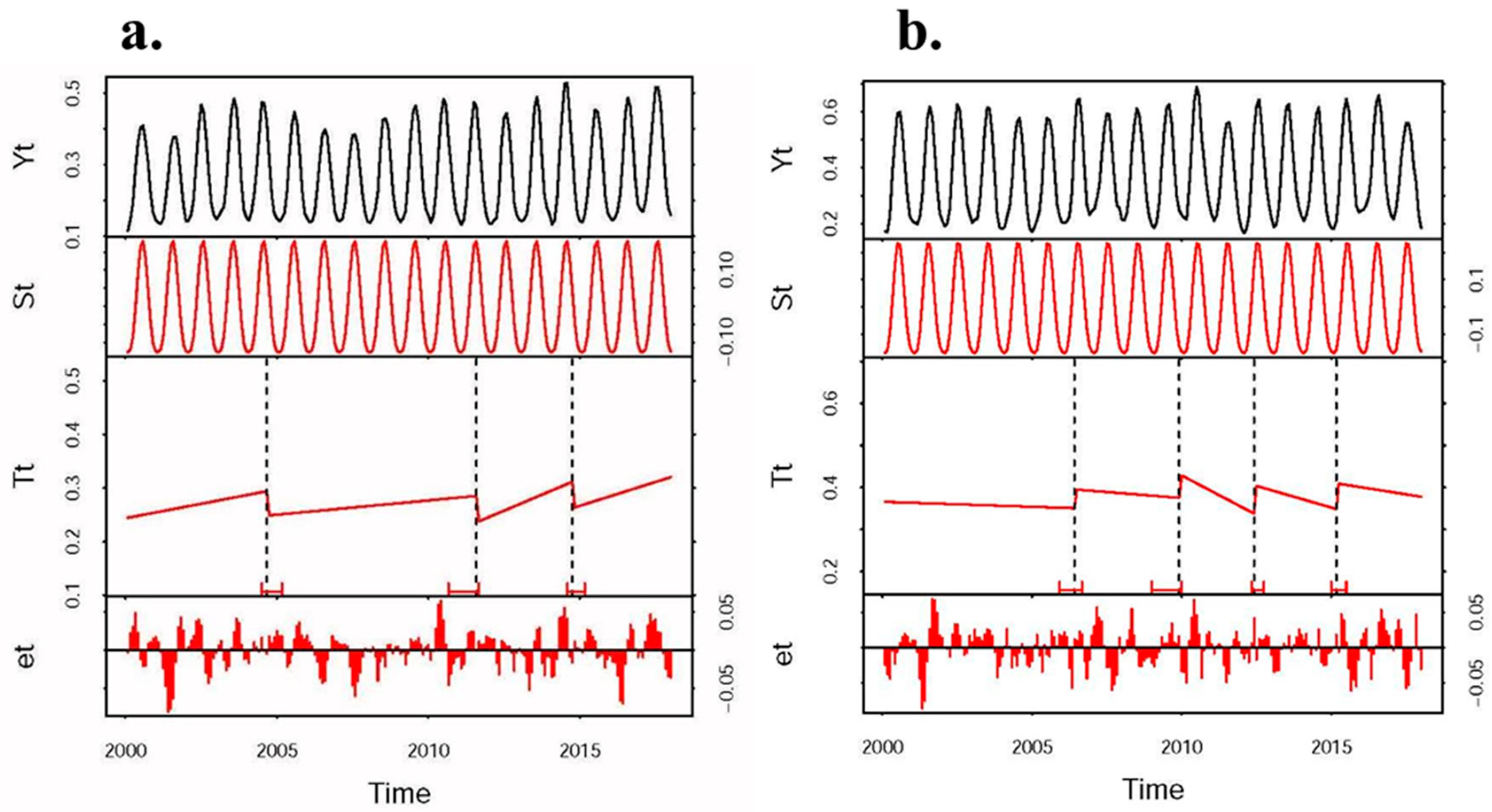
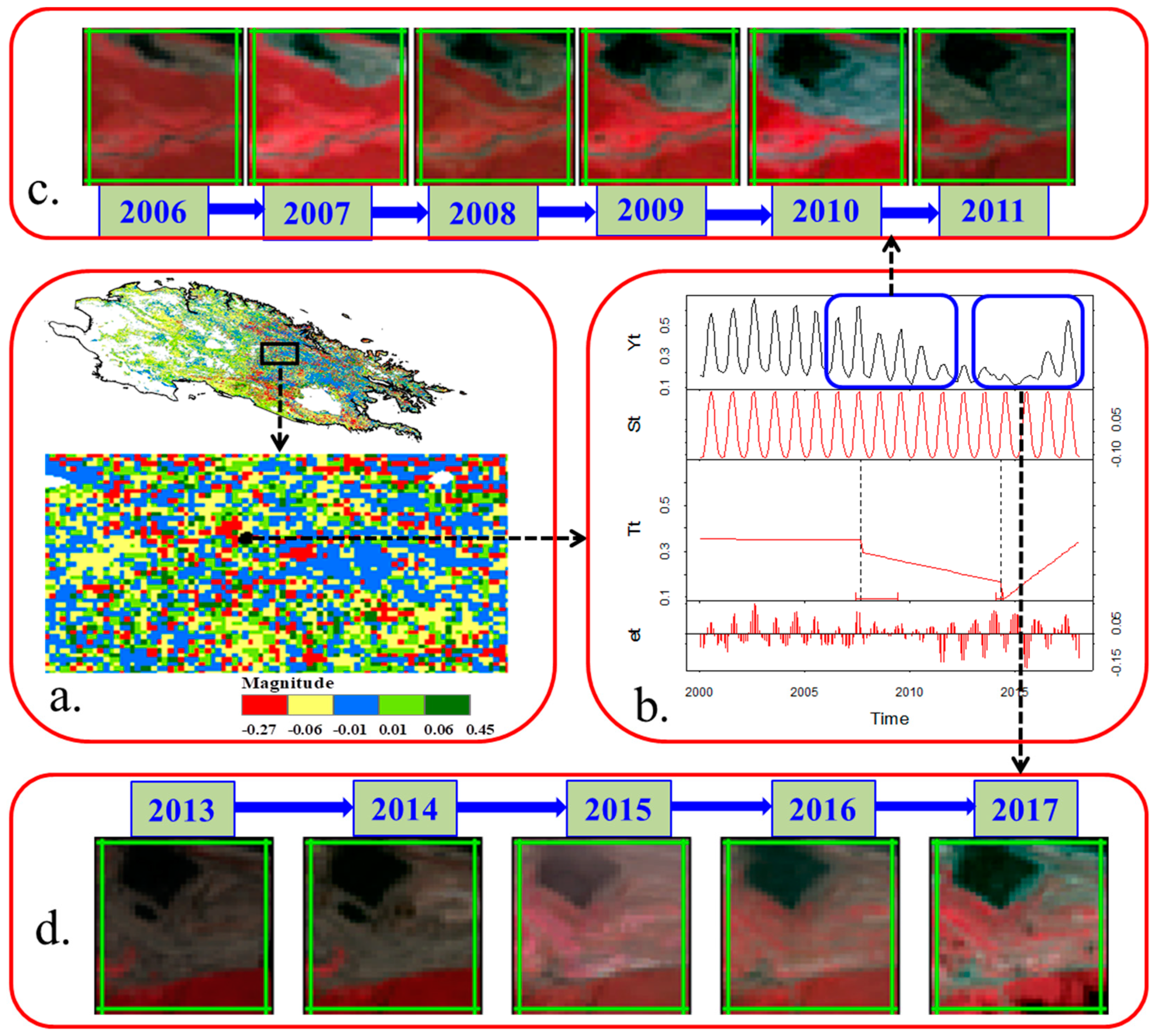
3.2. NDVI Dynamics Changes Based on BFAST
3.3. Linear Regression Analysis
4. Results
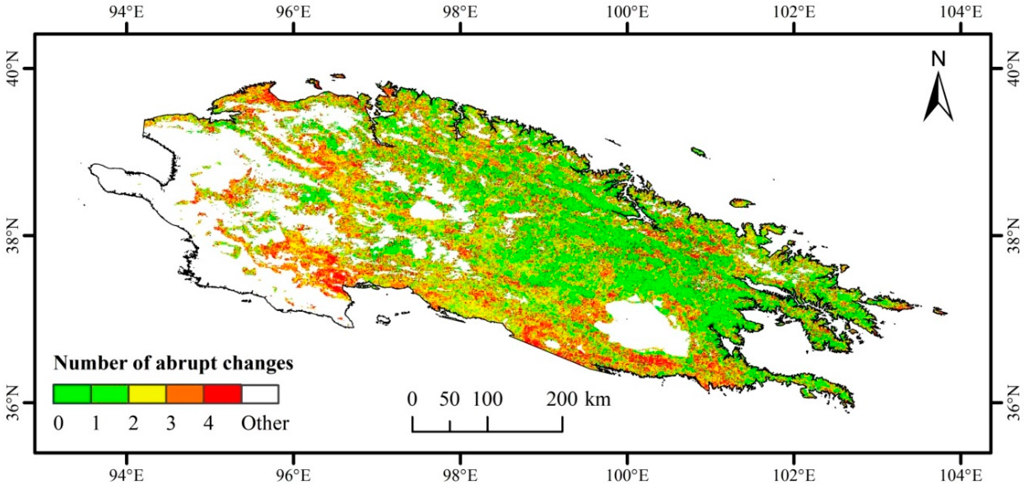
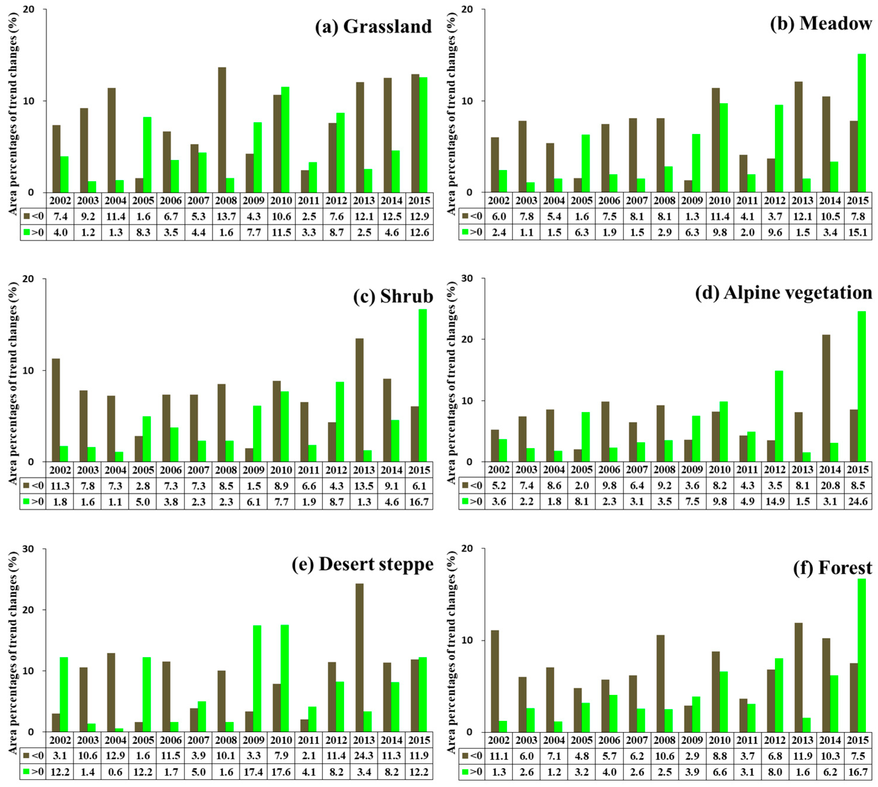
4.1. Number of Abrupt Changes
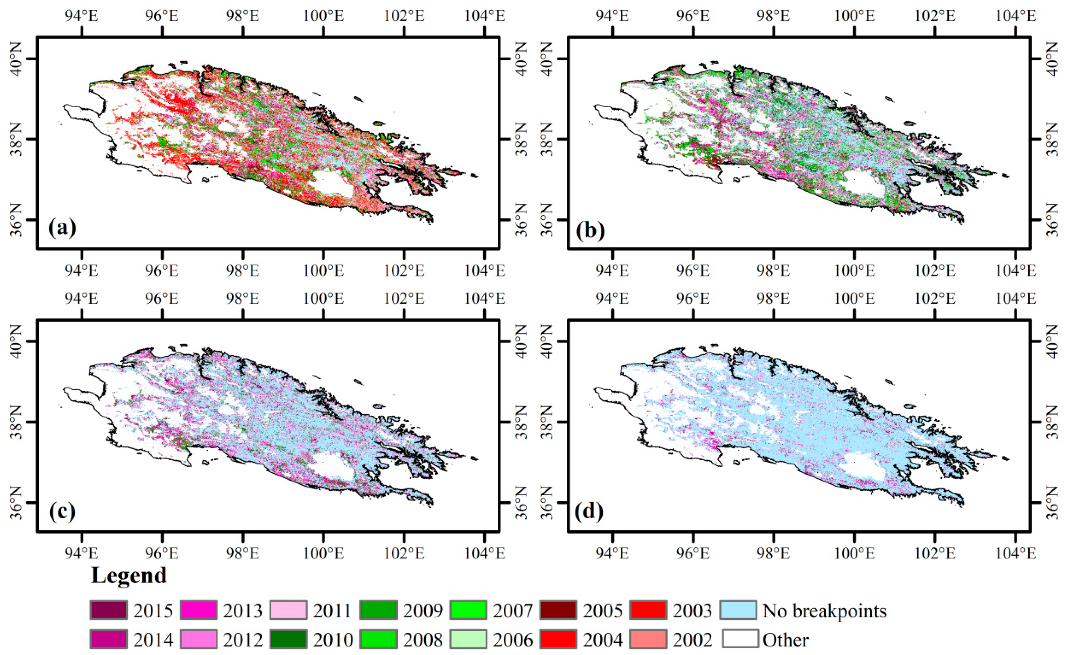
4.2. Timing of the Abrupt Changes
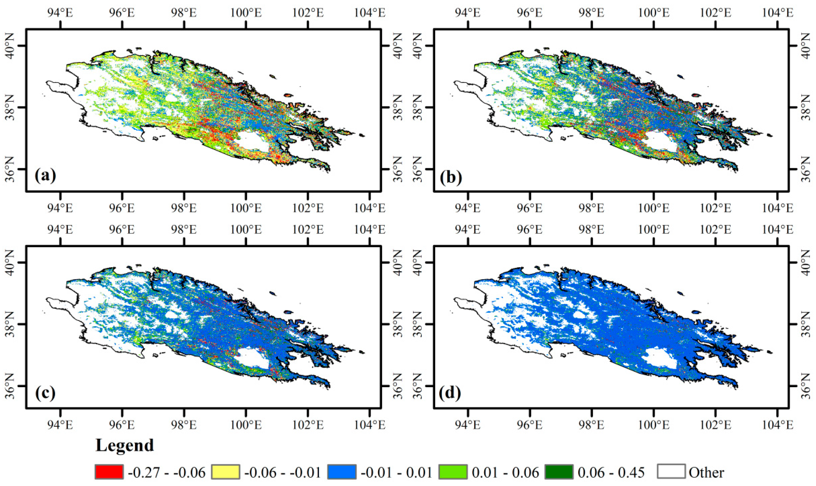
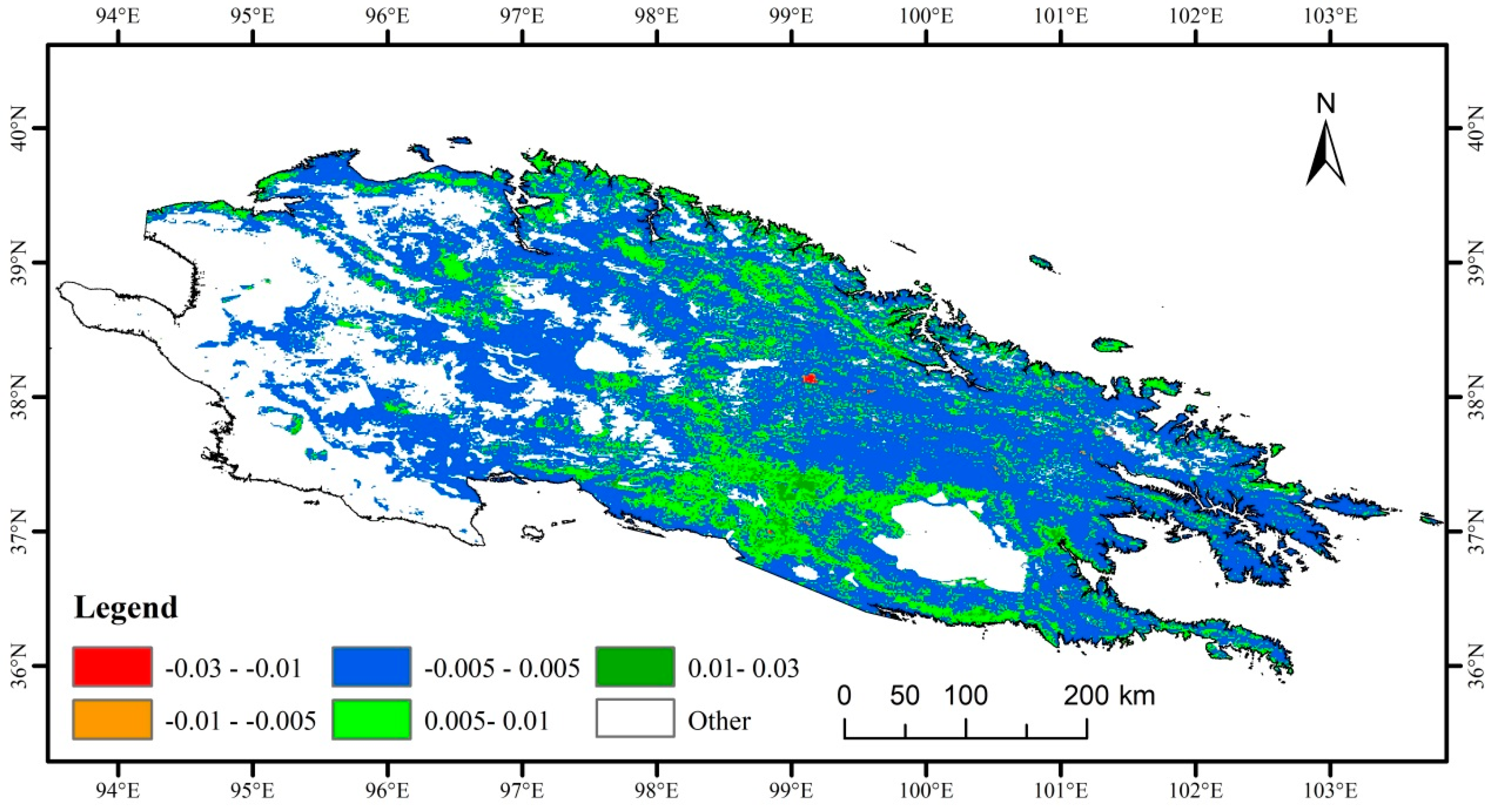
4.3. Magnitude of Abrupt Changes
5. Discussion
5.1. Effectiveness of the BFAST Model
5.2. Driving Factors Underlying Abrupt Vegetation Changes in the Qilian Mountains
6. Conclusions
Author Contributions
Funding
Acknowledgments
Conflicts of Interest
References
- Malmström, C.M.; Thompson, M.V.; Juday, G.P.; Los, S.O.; Randerson, J.T.; Field, C.B. Interannual variation in global-scale net primary production: Testing model estimates. Glob. Biogeochem. Cycles 1997, 11, 367–392. [Google Scholar] [CrossRef]
- Penuelas, J.; Rutishauser, T.; Filella, I. Phenology Feedbacks on Climate Change. Science 2009, 324, 887–888. [Google Scholar] [CrossRef] [PubMed]
- Hilker, T.; Lyapustin, A.I.; Tucker, C.J.; Hall, F.G.; Myneni, R.B.; Wang, Y.J.; Bi, J.; de Moura, Y.M.; Sellers, P.J. Vegetation dynamics and rainfall sensitivity of the Amazon. Proc. Natl. Acad. Sci. USA 2014, 111, 16041–16046. [Google Scholar] [CrossRef] [PubMed]
- Nemani, R.R.; Keeling, C.D.; Hashimoto, H.; Jolly, W.M.; Piper, S.C.; Tucker, C.J.; Myneni, R.B.; Running, S.W. Climate-driven increases in global terrestrial net primary production from 1982 to 1999. Science 2003, 300, 1560–1563. [Google Scholar] [CrossRef] [PubMed]
- Zhao, M.S.; Running, S.W. Drought-Induced Reduction in Global Terrestrial Net Primary Production from 2000 through 2009. Science 2010, 329, 940–943. [Google Scholar] [CrossRef]
- Piao, S.L.; Sitch, S.; Ciais, P.; Friedlingstein, P.; Peylin, P.; Wang, X.H.; Ahlstrom, A.; Anav, A.; Canadell, J.G.; Cong, N.; et al. Evaluation of terrestrial carbon cycle models for their response to climate variability and to CO2 trends. Glob. Chang. Biol. 2013, 19, 2117–2132. [Google Scholar] [CrossRef]
- Myneni, R.B.; Keeling, C.D.; Tucker, C.J.; Asrar, G.; Nemani, R.R. Increased plant growth in the northern high latitudes from 1981 to 1991. Nature 1997, 386, 698–702. [Google Scholar] [CrossRef]
- Chen, B.; Xu, G.; Coops, N.C.; Ciais, P.; Innes, J.L.; Wang, G.; Myneni, R.B.; Wang, T.; Krzyzanowski, J.; Li, Q.; et al. Changes in vegetation photosynthetic activity trends across the Asia-Pacific region over the last three decades. Remote Sens. Environ. 2014, 144, 28–41. [Google Scholar] [CrossRef]
- Wen, Z.; Wu, S.; Chen, J.; Lu, M. NDVI indicated long-term interannual changes in vegetation activities and their responses to climatic and anthropogenic factors in the Three Gorges Reservoir Region, China. Sci. Total Environ. 2017, 574, 947–959. [Google Scholar] [CrossRef]
- Zhang, Y.; Song, C.; Band, L.E.; Sun, G.; Li, J. Reanalysis of global terrestrial vegetation trends from MODIS products: Browning or greening? Remote Sens. Environ. 2017, 191, 145–155. [Google Scholar] [CrossRef]
- Zhang, Y.; Zhu, Z.; Liu, Z.; Zeng, Z.; Ciais, P.; Huang, M.; Liu, Y.; Piao, S. Seasonal and interannual changes in vegetation activity of tropical forests in Southeast Asia. Agric. For. Meteorol. 2016, 224, 1–10. [Google Scholar] [CrossRef]
- Pettorelli, N.; Vik, J.O.; Mysterud, A.; Gaillard, J.-M.; Tucker, C.J.; Stenseth, N.C. Using the satellite-derived NDVI to assess ecological responses to environmental change. Trends Ecol. Evol. 2005, 20, 503–510. [Google Scholar] [CrossRef] [PubMed]
- Kerr, J.T.; Ostrovsky, M. From space to species: Ecological applications for remote sensing. Trends Ecol. Evol. 2003, 18, 299–305. [Google Scholar] [CrossRef]
- Verbesselt, J.; Zeileis, A.; Herold, M. Near real-time disturbance detection using satellite image time series. Remote Sens. Environ. 2012, 123, 98–108. [Google Scholar] [CrossRef]
- Shen, M.; Piao, S.; Chen, X.; An, S.; Fu, Y.H.; Wang, S.; Cong, N.; Janssens, I.A. Strong impacts of daily minimum temperature on the green-up date and summer greenness of the Tibetan Plateau. Glob. Chang. Biol. 2016, 22, 3057–3066. [Google Scholar] [CrossRef] [PubMed]
- Liu, Q.; Fu, Y.H.; Zeng, Z.; Huang, M.; Li, X.; Piao, S. Temperature, precipitation, and insolation effects on autumn vegetation phenology in temperate China. Glob. Chang. Biol. 2016, 22, 644–655. [Google Scholar] [CrossRef] [PubMed]
- Shen, M.; Piao, S.; Cong, N.; Zhang, G.; Jassens, I.A. Precipitation impacts on vegetation spring phenology on the Tibetan Plateau. Glob. Chang. Biol. 2015, 21, 3647–3656. [Google Scholar] [CrossRef]
- Park, H.; Jeong, S.-J.; Ho, C.-H.; Kim, J.; Brown, M.E.; Schaepman, M.E. Nonlinear response of vegetation green-up to local temperature variations in temperate and boreal forests in the Northern Hemisphere. Remote Sens. Environ. 2015, 165, 100–108. [Google Scholar] [CrossRef]
- Cong, N.; Wang, T.; Nan, H.; Ma, Y.; Wang, X.; Myneni, R.B.; Piao, S. Changes in satellite-derived spring vegetation green-up date and its linkage to climate in China from 1982 to 2010: A multimethod analysis. Glob. Chang. Biol. 2013, 19, 881–891. [Google Scholar] [CrossRef]
- Piao, S.; Nan, H.; Huntingford, C.; Ciais, P.; Friedlingstein, P.; Sitch, S.; Peng, S.; Ahlstrom, A.; Canadell, J.G.; Cong, N.; et al. Evidence for a weakening relationship between interannual temperature variability and northern vegetation activity. Nat. Commun. 2014, 5. [Google Scholar] [CrossRef]
- Verbesselt, J.; Hyndman, R.; Zeileis, A.; Culvenor, D. Phenological change detection while accounting for abrupt and gradual trends in satellite image time series. Remote Sens. Environ. 2010, 114, 2970–2980. [Google Scholar] [CrossRef]
- Watts, L.M.; Laffan, S.W. Effectiveness of the BFAST algorithm for detecting vegetation response patterns in a semi-arid region. Remote Sens. Environ. 2014, 154, 234–245. [Google Scholar] [CrossRef]
- Kennedy, R.E.; Yang, Z.; Cohen, W.B. Detecting trends in forest disturbance and recovery using yearly Landsat time series: 1. LandTrendr—Temporal segmentation algorithms. Remote Sens. Environ. 2010, 114, 2897–2910. [Google Scholar] [CrossRef]
- Verbesselt, J.; Hyndman, R.; Newnham, G.; Culvenor, D. Detecting trend and seasonal changes in satellite image time series. Remote Sens. Environ. 2010, 114, 106–115. [Google Scholar] [CrossRef]
- Huang, C.; Goward, S.N.; Masek, J.G.; Thomas, N.; Zhu, Z.; Vogelmann, J.E. An automated approach for reconstructing recent forest disturbance history using dense Landsat time series stacks. Remote Sens. Environ. 2010, 114, 183–198. [Google Scholar] [CrossRef]
- Jamali, S.; Jönsson, P.; Eklundh, L.; Ardö, J.; Seaquist, J. Detecting changes in vegetation trends using time series segmentation. Remote Sens. Environ. 2015, 156, 182–195. [Google Scholar] [CrossRef]
- Schultz, M.; Clevers, J.G.P.W.; Carter, S.; Verbesselt, J.; Avitabile, V.; Quang, H.V.; Herold, M. Performance of vegetation indices from Landsat time series in deforestation monitoring. Int. J. Appl. Earth Obs. Geoinf. 2016, 52, 318–327. [Google Scholar] [CrossRef]
- Schmidt, M.; Lucas, R.; Bunting, P.; Verbesselt, J.; Armston, J. Multi-resolution time series imagery for forest disturbance and regrowth monitoring in Queensland, Australia. Remote Sens. Environ. 2015, 158, 156–168. [Google Scholar] [CrossRef]
- Chen, L.; Michishita, R.; Xu, B. Abrupt spatiotemporal land and water changes and their potential drivers in Poyang Lake, 2000–2012. ISPRS J. Photogramm. Remote Sens. 2014, 98, 85–93. [Google Scholar] [CrossRef]
- Tsutsumida, N.; Saizen, I.; Matsuoka, M.; Ishii, R. Land cover change detection in Ulaanbaatar using the breaks for additive seasonal and trend method. Land 2013, 2, 534–549. [Google Scholar] [CrossRef]
- Cheng, G.D.; Li, X.; Zhao, W.Z.; Xu, Z.M.; Feng, Q.; Xiao, S.C.; Xiao, H.L. Integrated study of the water-ecosystem-economy in the Heihe River Basin. Natl. Sci. Rev. 2014, 1, 413–428. [Google Scholar] [CrossRef]
- Li, X.; Cheng, G.; Liu, S.; Xiao, Q.; Ma, M.; Jin, R.; Che, T.; Liu, Q.; Wang, W.; Qi, Y. Heihe Watershed Allied Telemetry Experimental Research (HiWATER): Scientific objectives and experimental design. Bull. Am. Meteorol. Soc. 2013, 94, 1145–1160. [Google Scholar] [CrossRef]
- Tian, X.; Yan, M.; van der Tol, C.; Li, Z.; Su, Z.B.; Chen, E.X.; Li, X.; Li, L.H.; Wang, X.F.; Pan, X.D.; et al. Modeling forest above-ground biomass dynamics using multi-source data and incorporated models: A case study over the Qilian Mountains. Agric. For. Meteorol. 2017, 246, 1–14. [Google Scholar] [CrossRef]
- Wang, N.L.; Zhang, S.B.; He, J.Q.; Pu, J.C.; Wu, X.B.; Jiang, X. Tracing the major source area of the mountainous runoff generation of the Heihe River in northwest China using stable isotope technique. Chin. Sci. Bull. 2009, 54, 2751–2757. [Google Scholar] [CrossRef]
- Yang, W.J.; Wang, Y.H.; Wang, S.L.; Webb, A.A.; Yu, P.T.; Liu, X.D.; Zhang, X.L. Spatial distribution of Qinghai spruce forests and the thresholds of influencing factors in a small catchment, Qilian Mountains, northwest China. Sci. Rep. 2017, 7. [Google Scholar] [CrossRef] [PubMed]
- Sun, F.X.; Lyu, Y.H.; Fu, B.J.; Hu, J. Hydrological services by mountain ecosystems in Qilian Mountain of China: A review. Chin. Geogr. Sci. 2016, 26, 174–187. [Google Scholar] [CrossRef]
- Lin, P.; He, Z.; Du, J.; Chen, L.; Zhu, X.; Li, J. Recent changes in daily climate extremes in an arid mountain region, a case study in northwestern China’s Qilian Mountains. Sci. Rep. 2017, 7. [Google Scholar] [CrossRef]
- Du, J.; He, Z.; Yang, J.; Chen, L.; Zhu, X. Detecting the effects of climate change on canopy phenology in coniferous forests in semi-arid mountain regions of China. Int. J. Remote Sens. 2014, 35, 6490–6507. [Google Scholar] [CrossRef]
- Chen, J.; Jia, W.; Zhao, Z.; Zhang, Y.; Liu, Y. Research on Temporal and Spatial Variation Characteristics of Vegetation Cover in Qilian Mountains from 1982 to 2006. Adv. Earth Sci. 2015, 30, 834–845. [Google Scholar] [CrossRef]
- Wu, Z.; Jia, W.; Zhao, Z.; Zhang, Y.; Liu, Y.; Chen, J. Spatial-temporal variations of vegetation and its correlation with climatic factors in Qilian Mountains from 2000 to 2012. Arid Land Geogr. 2015, 38, 1241–1252. [Google Scholar]
- Wang, J.; Ye, B.; Liu, F.; Li, J.; Yang, G. Variations of NDVI Over Elevational Zones during the Past Two Decades and Climatic Controls in the Qilian Mountains, Northwestern China. Arct. Antarct. Alp. Res. 2011, 43, 127–136. [Google Scholar] [CrossRef]
- Zhang, H.; Peng, D.; Deng, R.; Wang, D.; Han, Y. Dynamic Change of Land Use in Qilian Mountains Based on Time-series Landsat Image. J. Beijing Univ. Technol. 2017, 43, 665–676. [Google Scholar]
- Editorial Committee for Vegetation Map of China. Vegetation Atlas of China; Science Press: Beijing, China, 2001. [Google Scholar]
- Fang, X.; Zhu, Q.; Ren, L.; Chen, H.; Wang, K.; Peng, C. Large-scale detection of vegetation dynamics and their potential drivers using MODIS images and BFAST: A case study in Quebec, Canada. Remote Sens. Environ. 2018, 206, 391–402. [Google Scholar] [CrossRef]
- Holben, B.N. Characteristics of maximum-value composite images from temporal AVHRR data. Int. J. Remote Sens. 1986, 7, 1417–1434. [Google Scholar] [CrossRef]
- Geng, L.; Ma, M.; Wang, X.; Yu, W.; Jia, S.; Wang, H. Comparison of Eight Techniques for Reconstructing Multi-Satellite Sensor Time-Series NDVI Data Sets in the Heihe River Basin, China. Remote Sens. 2014, 6, 2024–2049. [Google Scholar] [CrossRef]
- Hird, J.; Mcdermid, G. Noise reduction of NDVI time series: An empirical comparison of selected techniques. Remote Sens. Environ. 2009, 113, 248–258. [Google Scholar] [CrossRef]
- Park, S. Cloud and cloud shadow effects on the MODIS vegetation index composites of the Korean Peninsula. Int. J. Remote Sens. 2013, 34, 1234–1247. [Google Scholar] [CrossRef]
- Chen, J.; Jönsson, P.; Tamura, M.; Gu, Z.; Matsushita, B.; Eklundh, L. A simple method for reconstructing a high-quality NDVI time-series data set based on the Savitzky-Golay filter. Remote Sens. Environ. 2004, 91, 332–344. [Google Scholar] [CrossRef]
- Pan, N.; Feng, X.; Fu, B.; Wang, S.; Ji, F.; Pan, S. Increasing global vegetation browning hidden in overall vegetation greening: Insights from time-varying trends. Remote Sens. Environ. 2018, 214, 59–72. [Google Scholar] [CrossRef]
- Cleveland, R.; Cleveland, W.; McRae, J.; Terpenning, I. STL: A seasonal trend decomposition procedure based on loess. J. Off. Stat. 1990, 6, 3–33. [Google Scholar]
- Zeileis, A. A unified approach to structural change tests based on ML scores, F statistics, and OLS residuals. Econom. Rev. 2005, 24, 445–466. [Google Scholar] [CrossRef]
- Chen, B.; Zhang, X.; Tao, J.; Wu, J.; Wang, J.; Shi, P.; Zhang, Y.; Yu, C. The impact of climate change and anthropogenic activities on alpine grassland over the Qinghai-Tibet Plateau. Agric. For. Meteorol. 2014, 189–190, 11–18. [Google Scholar] [CrossRef]
- Sun, R.; Lu, Q.; Ma, S. The current ecological situation of Qinghai Qilian Mountain area and analysis of deterioration cause. Qinghai Prataculture 2009, 18, 19–26. [Google Scholar]
- Wang, T.; Gao, F.; Wang, B.; Wang, P.; Wang, Q.; Song, H.; Yin, C. Status and suggestions on ecological protection and restoration of Qilian Mountian. J. Glaciol. Geocryol. 2017, 39, 229–234. [Google Scholar]
- Alexandridis, T.K.; Oikonomakis, N.; Gitas, I.Z.; Eskridge, K.M.; Silleos, N.G. The performance of vegetation indices for operational monitoring of CORINE vegetation types. Int. J. Remote Sens. 2014, 35, 3268–3285. [Google Scholar] [CrossRef]
- Deng, S.F.; Yang, T.B.; Zeng, B.; Zhu, X.F.; Xu, H.J. Vegetation cover variation in the Qilian Mountains and its response to climate change in 2000-2011. J. Mt. Sci. 2013, 10, 1050–1062. [Google Scholar] [CrossRef]
- Yu, Z.; Liu, S.; Wang, J.; Sun, P.; Liu, W.; Hartley, D.S. Effects of seasonal snow on the growing season of temperate vegetation in China. Glob. Chang. Biol. 2013, 19, 2182–2195. [Google Scholar] [CrossRef]
- Wan, Y.F.; Gao, Q.Z.; Li, Y.; Qin, X.B.; Ganjurjav; Zhang, W.-n.; Ma, X.; Liu, S. Change of snow cover and its impact on alpine vegetation in the source regions of large rivers on the Qinghai-Tibetan Plateau, China. Arct. Antarct. Alpi. Res. 2014, 46, 632–644. [Google Scholar] [CrossRef]
- Xiao, J.F.; Zhou, Y.; Zhang, L. Contributions of natural and human factors to increases in vegetation productivity in China. Ecosphere 2015, 6. [Google Scholar] [CrossRef]
- Chen, H.; Zhu, Q.; Peng, C.; Wu, N.; Wang, Y.; Fang, X.; Gao, Y.; Zhu, D.; Yang, G.; Tian, J.; et al. The impacts of climate change and human activities on biogeochemical cycles on the Qinghai-Tibetan Plateau. Glob. Chang. Biol. 2013, 19, 2940–2955. [Google Scholar] [CrossRef]
- Mu, S.; Zhou, S.; Chen, Y.; Li, J.; Ju, W.; Odeh, I.O.A. Assessing the impact of restoration-induced land conversion and management alternatives on net primary productivity in Inner Mongolian grassland, China. Glob. Planet. Chang. 2013, 108, 29–41. [Google Scholar] [CrossRef]
- Cai, H.; Yang, X.; Xu, X. Human-induced grassland degradation/restoration in the central Tibetan Plateau: The effects of ecological protection and restoration projects. Ecol. Eng. 2015, 83, 112–119. [Google Scholar] [CrossRef]
- Cao, S.X.; Ma, H.; Yuan, W.P.; Wang, X. Interaction of ecological and social factors affects vegetation recovery in China. Biol. Conserv. 2014, 180, 270–277. [Google Scholar] [CrossRef]
- Petursdottir, T.; Arnalds, O.; Baker, S.; Montanarella, L.; Aradottir, A.L. A Social-Ecological System Approach to Analyze Stakeholders, Interactions within a Large-Scale Rangeland Restoration Program. Ecol. Soc. 2013, 18. [Google Scholar] [CrossRef]


| Number of Breakpoints | 0 | 1 | 2 | 3 | 4 | 1 or More | |
|---|---|---|---|---|---|---|---|
| Grassland | Pixels | 4685 | 5582 | 8179 | 7483 | 3205 | 24,449 |
| Proportion (%) | 16.08 | 19.16 | 28.07 | 25.68 | 11.00 | 83.92 | |
| Meadow | Pixels | 13,824 | 12,333 | 13,538 | 10,787 | 4707 | 41,365 |
| Proportion (%) | 25.05 | 22.35 | 24.53 | 19.55 | 8.53 | 74.95 | |
| Shrub | Pixels | 3490 | 3228 | 3732 | 2953 | 1383 | 11,296 |
| Proportion (%) | 23.60 | 21.83 | 25.24 | 19.97 | 9.35 | 76.40 | |
| Alpine vegetation | Pixels | 1531 | 1978 | 2608 | 2334 | 1130 | 8050 |
| Proportion (%) | 15.98 | 20.65 | 27.22 | 24.36 | 11.79 | 84.02 | |
| Desert steppe | Pixels | 975 | 2221 | 4642 | 4196 | 2171 | 13,230 |
| Proportion (%) | 6.86 | 15.64 | 32.68 | 29.54 | 15.28 | 93.14 | |
| Forest | Pixels | 453 | 623 | 632 | 485 | 185 | 1925 |
| Proportion (%) | 19.05 | 26.20 | 26.58 | 20.40 | 7.78 | 80.95 | |
| All study vegetation | Pixels | 24,958 | 25,965 | 33,331 | 28,238 | 12,781 | 10,0315 |
| Proportion (%) | 19.92 | 20.73 | 26.61 | 22.54 | 10.20 | 80.08 | |
| Years | Grassland | Meadow | Shrub | Alpine Vegetation | Desert Steppe | Forest | All Study Vegetation |
|---|---|---|---|---|---|---|---|
| 2002 | 11.32 | 8.46 | 13.05 | 8.84 | 15.28 | 12.36 | 10.54 |
| 2003 | 10.43 | 8.87 | 9.44 | 9.55 | 11.93 | 8.62 | 9.70 |
| 2004 | 12.74 | 6.90 | 8.33 | 10.35 | 13.50 | 8.24 | 9.47 |
| 2005 | 9.85 | 7.89 | 7.79 | 10.07 | 13.82 | 8.03 | 9.18 |
| 2006 | 10.19 | 9.43 | 11.11 | 12.15 | 13.20 | 9.76 | 10.45 |
| 2007 | 9.66 | 9.60 | 9.66 | 9.54 | 8.90 | 8.75 | 9.52 |
| 2008 | 15.25 | 10.94 | 10.78 | 12.73 | 11.72 | 13.08 | 12.19 |
| 2009 | 11.93 | 7.65 | 7.60 | 11.13 | 20.75 | 6.81 | 10.38 |
| 2010 | 22.16 | 21.16 | 16.60 | 18.03 | 25.49 | 15.39 | 20.99 |
| 2011 | 5.78 | 6.06 | 8.41 | 9.16 | 6.17 | 6.73 | 6.54 |
| 2012 | 16.29 | 13.29 | 13.07 | 18.36 | 19.63 | 14.84 | 15.10 |
| 2013 | 14.60 | 13.56 | 14.74 | 9.55 | 27.69 | 13.46 | 15.24 |
| 2014 | 17.12 | 13.83 | 13.65 | 23.85 | 19.51 | 16.48 | 16.03 |
| 2015 | 25.46 | 22.96 | 22.74 | 33.06 | 24.13 | 24.22 | 24.45 |
| Vegetation | Breakpoints | −0.27 to −0.06 | −0.06 to −0.01 | −0.01 to 0.01 | 0.01 to 0.06 | 0.06 to 0.45 |
|---|---|---|---|---|---|---|
| Grassland | 1 | 8.69 | 45.51 | 18.58 | 22.41 | 4.80 |
| 2 | 8.77 | 26.73 | 38.53 | 21.30 | 4.68 | |
| 3 | 4.90 | 15.02 | 65.25 | 12.17 | 2.66 | |
| 4 | 1.07 | 4.45 | 90.05 | 3.72 | 0.71 | |
| Meadow | 1 | 13.75 | 34.36 | 26.98 | 18.93 | 5.98 |
| 2 | 11.58 | 17.68 | 48.53 | 13.23 | 8.98 | |
| 3 | 5.33 | 8.66 | 72.74 | 7.67 | 5.60 | |
| 4 | 1.42 | 2.45 | 91.75 | 2.46 | 1.92 | |
| Shrub | 1 | 17.59 | 36.06 | 24.74 | 14.96 | 6.64 |
| 2 | 13.21 | 17.31 | 45.87 | 13.01 | 10.60 | |
| 3 | 6.88 | 7.21 | 71.58 | 7.42 | 6.91 | |
| 4 | 2.02 | 2.16 | 91.13 | 2.46 | 2.24 | |
| Alpine vegetation | 1 | 8.70 | 40.50 | 17.25 | 26.31 | 7.23 |
| 2 | 8.91 | 23.37 | 37.79 | 21.23 | 8.71 | |
| 3 | 4.16 | 12.71 | 64.43 | 13.51 | 5.19 | |
| 4 | 1.25 | 3.95 | 88.54 | 4.21 | 2.05 | |
| Desert steppe | 1 | 2.35 | 45.45 | 17.10 | 33.12 | 1.97 |
| 2 | 3.03 | 29.73 | 33.95 | 30.76 | 2.52 | |
| 3 | 1.37 | 17.78 | 63.51 | 16.13 | 1.21 | |
| 4 | 0.34 | 5.61 | 88.35 | 5.22 | 0.48 | |
| Forest | 1 | 18.76 | 37.83 | 19.47 | 15.03 | 8.91 |
| 2 | 16.18 | 15.02 | 45.23 | 13.12 | 10.44 | |
| 3 | 7.68 | 7.16 | 71.47 | 7.42 | 6.26 | |
| 4 | 2.72 | 1.81 | 91.41 | 1.86 | 2.20 | |
| All study vegetation | 1 | 11.40 | 38.98 | 22.73 | 21.42 | 5.47 |
| 2 | 10.02 | 21.50 | 43.34 | 17.69 | 7.44 | |
| 3 | 4.91 | 11.29 | 69.15 | 10.10 | 4.55 | |
| 4 | 1.30 | 3.34 | 90.64 | 3.19 | 1.53 |
| Years | Negative Change (Abrupt Browning) (%) | Positive Change (Abrupt Greening) (%) | Stable (%) |
|---|---|---|---|
| 2002 | 6.65 | 3.89 | 89.46 |
| 2003 | 8.37 | 1.33 | 90.30 |
| 2004 | 8.13 | 1.33 | 90.53 |
| 2005 | 1.82 | 7.36 | 90.82 |
| 2006 | 7.88 | 2.56 | 89.55 |
| 2007 | 6.72 | 2.80 | 90.48 |
| 2008 | 9.80 | 2.39 | 87.81 |
| 2009 | 2.45 | 7.93 | 89.62 |
| 2010 | 10.24 | 10.75 | 79.01 |
| 2011 | 3.78 | 2.75 | 93.46 |
| 2012 | 5.61 | 9.49 | 84.90 |
| 2013 | 13.32 | 1.92 | 84.76 |
| 2014 | 11.67 | 4.36 | 83.97 |
| 2015 | 9.31 | 15.14 | 75.55 |
© 2019 by the authors. Licensee MDPI, Basel, Switzerland. This article is an open access article distributed under the terms and conditions of the Creative Commons Attribution (CC BY) license (http://creativecommons.org/licenses/by/4.0/).
Share and Cite
Geng, L.; Che, T.; Wang, X.; Wang, H. Detecting Spatiotemporal Changes in Vegetation with the BFAST Model in the Qilian Mountain Region during 2000–2017. Remote Sens. 2019, 11, 103. https://doi.org/10.3390/rs11020103
Geng L, Che T, Wang X, Wang H. Detecting Spatiotemporal Changes in Vegetation with the BFAST Model in the Qilian Mountain Region during 2000–2017. Remote Sensing. 2019; 11(2):103. https://doi.org/10.3390/rs11020103
Chicago/Turabian StyleGeng, Liying, Tao Che, Xufeng Wang, and Haibo Wang. 2019. "Detecting Spatiotemporal Changes in Vegetation with the BFAST Model in the Qilian Mountain Region during 2000–2017" Remote Sensing 11, no. 2: 103. https://doi.org/10.3390/rs11020103
APA StyleGeng, L., Che, T., Wang, X., & Wang, H. (2019). Detecting Spatiotemporal Changes in Vegetation with the BFAST Model in the Qilian Mountain Region during 2000–2017. Remote Sensing, 11(2), 103. https://doi.org/10.3390/rs11020103