Rain Monitoring with Polarimetric GNSS Signals: Ground-Based Experimental Research

Abstract

In recent years, there has been a preliminary research on monitoring rainfall information based on polarimetric Global Navigation Satellite System (GNSS) signals, which is a quite novel concept. After previous theoretical research on monitoring rain based on polarimetric phase shift of GNSS signals, the paper aims to detect rain using polarimetric GNSS signals from a ground-based experiment. Firstly, a conical horn antenna specially designed for receiving dual-polarized (H, horizontal, and V, vertical) GNSS signals was developed, and an experimental system for polarimetric GNSS rain detection was built. Then, taking Global Positioning System (GPS) satellites as signal source, a ground-based experiment was carried out at a mountain in Nanjing, where heavy rain tends to occur frequently in rainy season. Additionally, a data processing algorithm mainly following Padullés et al. (2016) to solve the problems of quality control, unlocking, hardware effect, phase ambiguity, multipath effect was applied independently to this ground-based data from the polarimetric GNSS rain detection system. Also, the multi-source data from nearby weather radar and weather stations was used for verification. Results from 14 GPS satellites show that the obtained phase shift is zero in all no-rain days while it is not zero during rainy days, which is in accordance with the actual situation. Compared with weather radar and rain gauges’ data, the results verify that the phase shift is caused by rain. Besides, when individual cases are examined, many show that their tendencies of accumulated phase shift are quite similar to that of a weather station’s rainfall data, even some correlation coefficients are up to 0.99. These demonstrate the reliability of our experimental system and the feasibility of the data processing algorithm. This study will provide technical support for future spaceborne experiment, which has promising applications in global rain monitoring.

1. Introduction

Rain, a common weather phenomena, reflects the physical and chemical processes of atmospheric dynamics, thermodynamics and water vapor cycle [1]. It also plays an important role in transportation of atmospheric energy and global hydrologic cycle. However, its changing spatial and temporal distribution often leads to natural disasters such as floods and droughts [2]. Therefore, its forecasting, monitoring, and estimation is crucial for the research of scientific issues such as atmospheric dynamic analysis, numerical weather forecasting, weather and climate change, global water balance, hydrological model construction, meteorological disaster forecasting, flood disaster monitoring, and agricultural flood control et al. [3,4,5].

Traditionally, rain monitoring mostly relies on rain gauge, weather radar and satellite remote sensing [6]. Obviously, rain gauge, which is widely utilized, can provide accurate “point” measurement. The network of many rain gauge stations can be used to get regional rain rate by interpolation [7]. Regional rain information can also be obtained from weather radar based on its parameters such as radar reflectivity (Z), differential reflectivity (Z_DR) and specific differential phase shift (K_DP) [8,9,10]. Especially, these radar polarization parameters, Z_DR and K_DP offer more microscopic information about rain [11]. Additionally, remote sensing data from spaceborne payloads such as infrared/visible sensors on Geosynchronous Earth Orbit satellites, passive microwave sensors and precipitation radar on Low Earth Orbit satellites has capable of yielding rain information [5,12]. Then, some spaceborne rain products including the Climate Prediction Center Morphing technique product (CMORPH) [13], the Tropical Rainfall Measuring Mission (TRMM) Multi-satellite Precipitation Analysis [14], Global Satellite Mapping of Precipitation (GSMaP) [15] are produced.

Recently, several novel methods based on microwave link signals are being developed to achieve rain information. When propagating though rain area, microwave link signals, usually come across attenuation and depolarization, which is a problem for communication. However, it is beneficial for meteorology. Some researchers have found it is possible to estimate rain rate using rain-induced attenuation [16,17]. Path-averaged rain rate was studied in theory and experiments according to the relationship between microwave attenuation and rain rate [16]. The feasibility of monitoring rain using wireless communication networks was investigated by Messer et al. [18]. Based on the cellular wireless network covering all parts of the Netherlands, more than 2400 links of rain attenuation were obtained through experiments, and country-wide rainfall maps were retrieved [19]. A microwave link experiment was also set up to assess several error sources associated with rain rate estimation from cellular communication networks [20]. Besides, in 2018, the feasibility of rain detection over oceans by Global Navigation Satellite System (GNSS) reflectometry observations was firstly investigated at weak winds [21].

Rain-induced depolarization can also be used to obtain rain information. A polarimetric concept that uses the depolarization of GNSS signals to detect heavy rain was first proposed by Cardellach et al. [22]. Then, they did some theoretical research to assess the sensitivity of GNSS signals for remote sensing of heavy rain [23]. A field campaign was also carried out to investigate the detectability of polarimetric phase shift and the feasibility of estimating rain information [24]. These research intended to solve some problems for the the Radio-Occultation and Heavy Precipitation (ROHP) experiment aboard the Spanish Earth Observation satellite PAZ. An and Yan et al. [12,25] also conducted some research on the physical process of GNSS signals propagating through rain-filled medium and the relationships between cross-polarization discrimination, polarimetric phase shift and rain rate, respectively. Recently, the Spanish satellite PAZ has been launched successfully in 2018 [26]. However, this concept is still under research.

Based on previous theoretical research [12,25], a ground-based experiment was conducted to study the feasibility of this concept. This experiment was carried out on a mountain to receive GNSS signals in grazing angle geometry [25]. A long term observation was implemented in order to collect a large number of data on no-rain days and catch more cases in rainy days to study the phase difference between horizontal and vertical GNSS signals. At the same time, nearby weather radar and weather station data was also collected.

The major objectives of this study are to verify the reliability of our experimental system, which was specially designed for receiving dual-polarized GNSS signals and solve a series of problems related to data processing. For this purpose, the methodology of Padullés et al. [24], for radio-occultation data, is applied to this ground-based data records. Section 2 gives an overview of the experiment and details the data processing algorithm about how to solve quality control, unlocking, hardware effect, phase ambiguity, multipath effect and identify phase shift. The statistical results of no-rain and rainy days and comparison results of rainy cases with weather radar and weather station data are analysed and discussed systematically in Section 3. Finally, some conclusions are summarized in Section 4.

2. Experiments and Data

2.1. Mechanism of Detection

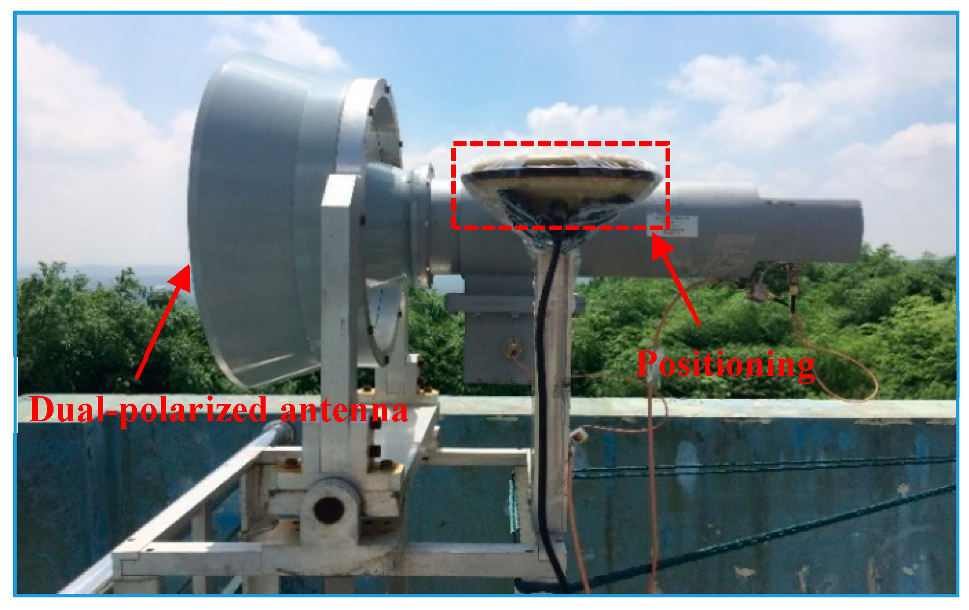
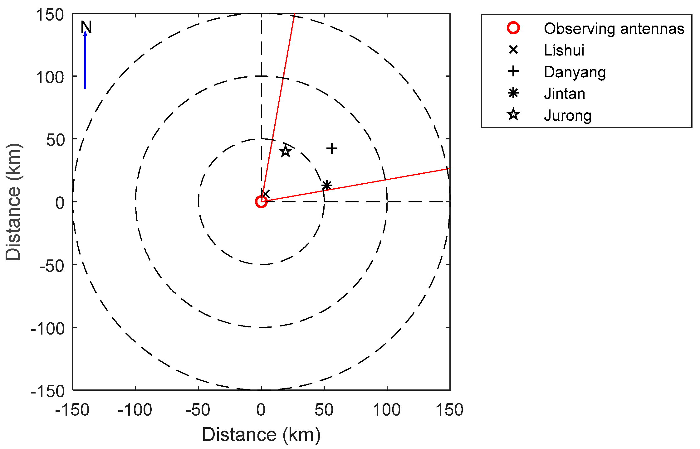
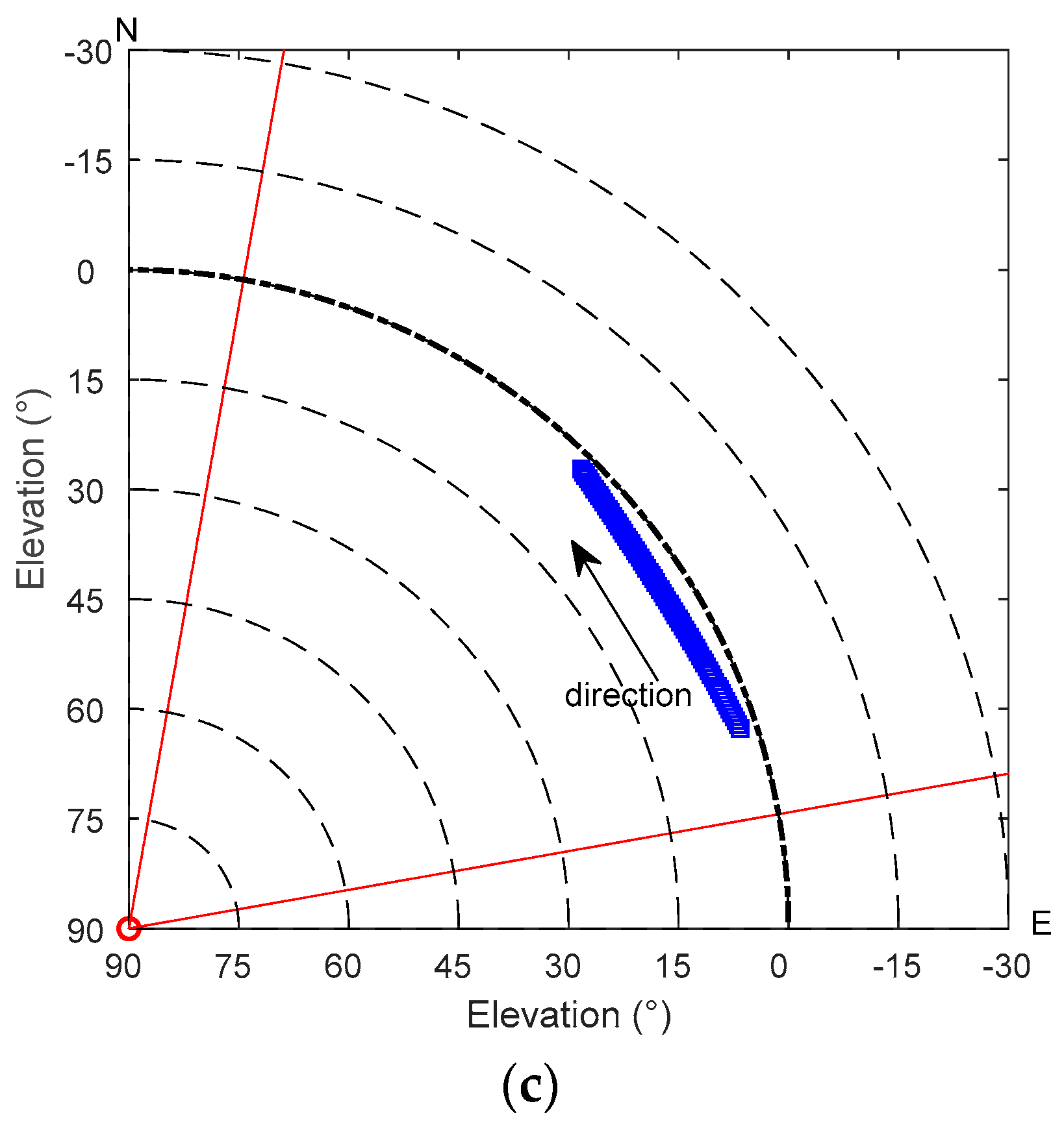
Since the shapes of falling raindrops are always nonspherical, the depolarization of GNSS signals is inevitable when it passes through rain area [25]. Polarimetric phase shift, which is used to describe depolarization characteristic, is defined as

$$\Delta \varphi ={\varphi }_h-{\varphi }_v$$

(1)

where ${\varphi }_h$ and ${\varphi }_v$ is the horizontally and vertically polarized phases, respectively. In theory, the polarimetric phase shift, can be obtained from

$$\Delta \varphi ={\displaystyle {\int }_L{K}_{DP}dl}$$

(2)

where L is the path length through rain area; $K_{DP}$ is the specific differential phase, which is related to rain rate and more specifically to the characteristics of rain particles. However, the $K_{DP}$ here comes from forward-scattering of particles rather than back-scattering of particles. For a polarimetric weather radar, whose signals are always in S-, C-, or X-band, its $K_{DP}$ can be observed [8,9]. Here, the detectability of $K_{DP}$ from L-band signals is uncertain. Thus, an experiment is necessary and essential.

2.2. Experiments

From Equation (1), it can be seen that the horizontally and vertically polarized phases of GNSS signals should be received. However, there is no relevant equipment on the market now. Therefore, some devices have to be designed to receive dual-polarized GNSS signals with higher accuracy of phase measurement. Since receiving technology of GPS signals is relatively mature and its L1 (1.57542 GHz) is larger, L1 signal is regarded as our signal resource. A GNSS dual-polarized rain detection system is fabricated for the experiment, which consists of a GNSS dual-polarized receiving antenna, a dual-polarized receiver and a positioning antenna. The dual-polarized antenna is a conical horn antenna, developed by National Space Science Center, Chinese Academy of Science (NSSC-CAS) (see Figure 1) based on two vertical waveguides to receive horizontally and vertically polarized GNSS signals, respectively. Under this structure, the antenna patterns of horizontal polarization and vertical polarization have good consistency. The dual-polarized receiver is also supplied by NSSC-CAS, which is similar to the receiver of its GNSS occultation sounder (GNOS) onboard the FengYun 3 series C satellite [27]. The carrier phase and signal amplitude of horizontally and vertically polarized GPS signals can be obtained separately based on this kind of receiver. The positioning antenna is an ordinary omni-directional antenna produced by the manufacturer NovAtel in order to get accurate location of the receiving antenna.

This experiment is implemented at a mountain in Nanjing where heavy rain occurs frequently during annual rainy season. Fortunately, a weather radar station is at the top of the mountain, where has an S-band dual-polarized doppler weather radar. The receiver and receiving terminal (computer and receiving software) are sheltered in a room, not far from the antenna. The dual-polarized antenna points to the northeast horizon, which can track all visible satellites simultaneously in the north-east field of view from 10° to 80° of azimuth and −3° to 45° of elevation (see Figure 2, enclosed by red dashed line). Through the view, the antenna can receive signals from 22 GPS satellites (G1, G3, G7, G8, G9, G10, G11, G12, G13, G15, G16, G21, G22, G23, G24, G25, G26, G27, G28, G29, G30, G32) almost every day. However, observing period of each day is almost the same for a satellite but different for 22 satellites, ranging from several minutes to several hours. In Figure 2, the pointing triangle and downward pointing triangle represent ascending and descending GPS satellite respectively. The experiment is carried out twice, one from June to September in 2015 and the other one from July to November in 2016.

2.3. Data Processing Algorithm

2.3.1. Observation Equation

Observation from our GPS receiver is pseudo-range and carrier phase. However, data from horizontally and vertically polarized (H-pol, V-pol) signals are observed independently by the dual-polarized antenna and tracked separately by the receiver. The polarimetric phase shift is the carrier phase difference between H-pol and V-pol phase. The observation equation of carrier phase can be expressed as [24]

$$\varphi (t)=\rho (t)+{\rho }_{atm}(t)+{\rho }_{hyd}^{}(t)+{\rho }_{ion}(t)+m(t)+d+C(t)+b$$

(3)

where $\rho$ is the geometry distance between GPS satellite and the receiver, which is equal for H-pol and V-pol signals; ${\rho }_{atm}$ represents the phase delay induced by neutral atmosphere (the same for H-pol and V-pol signals); ${\rho }_{hyd}$ denotes the phase delay due to hydrometeors along the transmission path; ${\rho }_{ion}$ is the ionospheric delay; m denotes local multipath effect on each signal; d represents the hardware effect; C refers to the clock drifts and errors of the satellite; the term b denotes phase ambiguity, which is an arbitrary initial constant for each signal; t is the time.

Therefore, the carrier phase difference is

$$\Delta \varphi (t)={\varphi }_H(t)-{\varphi }_V(t)={\rho }_{hyd}^H(t)-{\rho }_{hyd}^V(t)+\Delta m+\Delta d+\Delta b$$

(4)

where $\Delta m=m^H-m^V$, $\Delta d=d^H-d^V$, $\Delta b=b^H-b^V$.

Based on Equation (4), the geometry distance and effect of neutral atmosphere, ionosphere, clock drifts and errors can be eliminated. However, those problems such as hardware effect, phase ambiguity and multipath effect should be further solved.

2.3.2. Method to Solve Hardware Effect and Phase Ambiguity

The hardware effect, namely the effect of transmitter and receiver, is basically the same during a process of receiving GPS signals. Thus, ∆d is a constant for an observation process. The ambiguity is also constant during a continuous period of data record, and then that Δb is constant [24]. Due to the fact that the observation of phase is not absolute, but relative to the initial value, the GPS receiver cannot get real phase value [28]. Furthermore, when its track is lost, the GPS receiver starts again with a new arbitrary initial value. Therefore, the longest continuous sequence in every day is used.

The orbital period of a GPS satellite is one sidereal day, which means that the satellite will be in the same position after a sidereal day. Thus, we can convert time series of observing data into elevation or azimuth series. Then, the same elevation or azimuth can be selected to ensure consistency of the initial data in every day. This transformation makes the data only depends on the position of GPS satellite. Since the absolute values of each data sequence depend on its initial value, each sequence minus its own mean is considered in order to compare different observing data [24]. At the same time, the hardware effect and phase ambiguity can be cancelled out using the following equation:

$$\Delta {\varphi }^{\prime }\left(\beta \right)=\Delta \varphi \left(\beta \right)-\langle \Delta \varphi \left(\beta \right)\rangle$$

(5)

where $\beta$ represents the trajectory of the GPS satellite defined by its elevation and azimuth.

2.3.3. Method to Deal with Multipath Effect

Multipath effect is a source of error for GNSS applications, which affects carrier phase measurements [29]. If GNSS signal falls on the ground before reaching a receiver, the reflection occurs. Thus, this signal may arrive at an antenna finally. In this situation, the receiver combines records of direct signals with multipath artefacts [30]. Since our polarized antenna is on the ground and its gazing angle is at the horizontal direction, multipath effect is inevitable.

The multipath effect is related to the environment in which the GPS receiver is located. Thus, the characteristic of multipath effect on the signal is stable in the same condition. This means that the term ∆m of a satellite should repeat after a sidereal day. Therefore, the ∆m can be regarded as background data. Its feature can be shown by average and standard deviation, which can be calculated as a function of angle $\beta$ from no-rain days. To get more accurate multipath feature, all the no-rain days’ data are used. Here, multipath effect can be removed by

$$\Delta {\varphi }^{″}\left(\beta \right)=\Delta {\varphi }^{\prime }\left(\beta \right)-\overline{\Delta m\left(\beta \right)}$$

(6)

where the mean ∆m over a sidereal day is obtained over the period of non-rainy days, which depends on the trajectory of the satellite and the surrounding of the instrument [24].

2.3.4. Method to Identify Phase Shift Induced by Raindrops

For each satellite, data from rainy days also suffers from multipath effect. We compare each $\Delta {\varphi }^{\prime }(\beta )$ with the standard deviation of Δm (${\sigma }_{\Delta m}$) to analyze the effect of hydrometeors. Here, we use “$2\sigma$” principle to obtain phase shift: 95% of the data should be within $\pm 2\sigma$ in statistics, the other 5% ought to exceed $\pm 2\sigma$ [24]. Since there is no absolute reference for phase shift, $\pm 2\sigma$ is a threshold. The minimal value where the difference is between $\Delta {\varphi }^{″}(\beta )$ and $-2\sigma$ can be calculated. Then, compute each $\Delta {\varphi }^{″}(\beta )$ by the equation:

$$\Delta {\varphi }_C(\beta )=\Delta {\varphi }^{″}(\beta )-{\left(\Delta {\varphi }^{″}(\beta )+2\sigma (\beta )\right)}_{\min }$$

(7)

Here, considering $+2\sigma$ as the no-rain noise level, the $\Delta {\varphi }_C(\beta )$ can be understood as corrected phase shift. Its value that surpass $+2\sigma$ is regarded as phase shift induced by hydrometeors and can be obtained from:

$$\Delta {\varphi }_{+}(\beta )=\{\begin{array}{ll}\Delta {\varphi }_C(\beta )-2\sigma (\beta )& \Delta {\varphi }_C(\beta )>2\sigma (\beta )\\ 0& \Delta {\varphi }_C(\beta )\le 2\sigma (\beta )\end{array}$$

(8)

where $\Delta {\varphi }_{+}(\beta )$ is a relative phase shift beyond the no-rain noise level. Its positive value comes from the contribution of hydrometeors, which includes not only raindrops but also ice crystals and melting particles. From our previous research, due to the fact that the number concentration of ice particles is often sparse at high altitude, the effect of ice crystals along the path is quite weak, which can be neglected [25]. Compared with the effect of larger and more concentrated raindrops, the melting particles have some effect but not that obvious. Besides, the effect of ionosphere has been also assessed. Its phase delays, Faraday rotation and Cotton–Mouton effects all have no influence on our measurements [25].

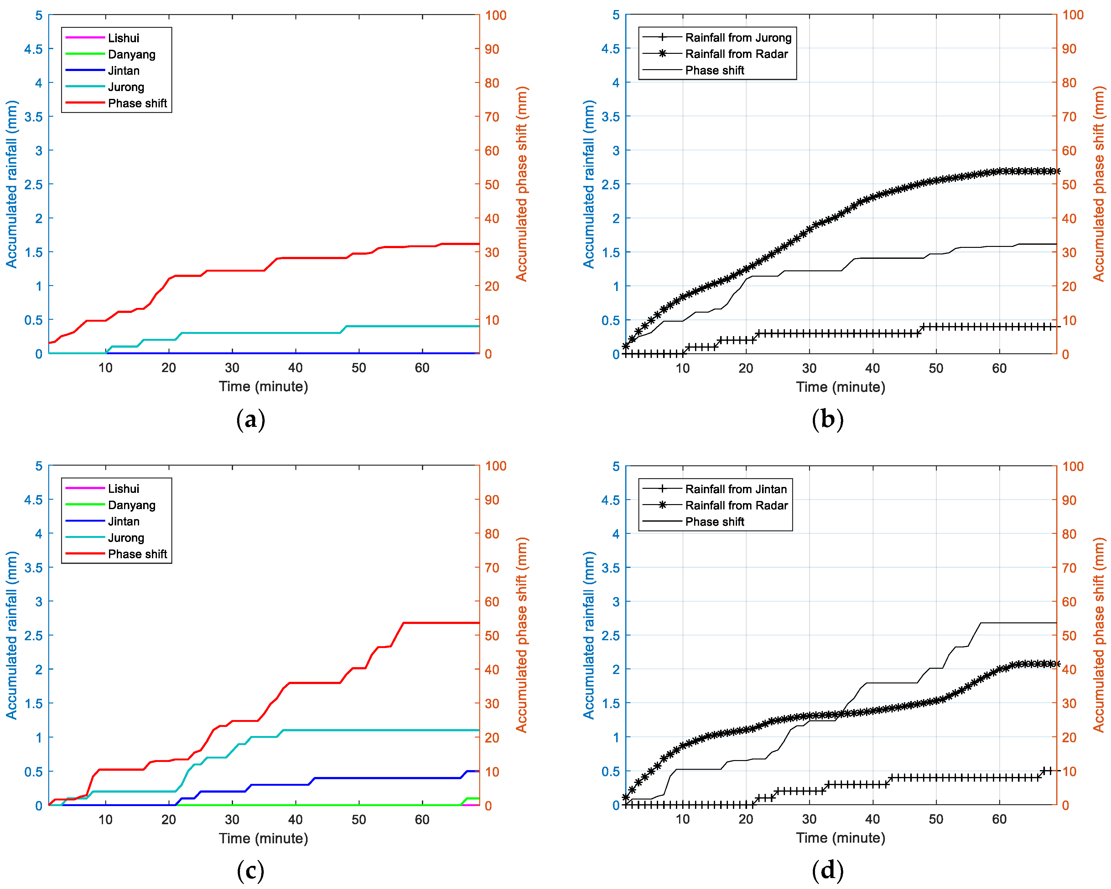
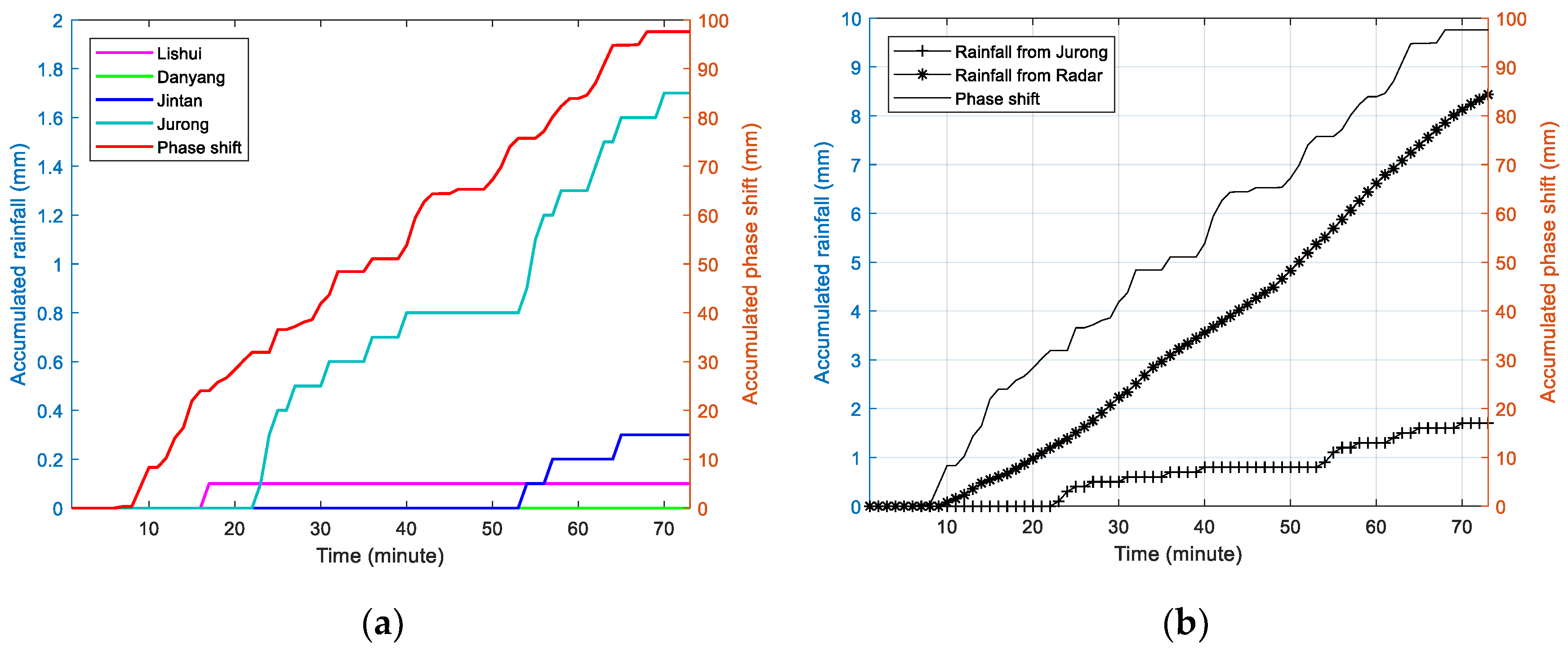
2.3.5. Comparison with Multi-Source Data

From Equation (8), the $\Delta {\varphi }_{+}(\beta )$ is expected to be caused by rain. Whether there are some raindrops just along the path requires other observations to verify. The data of the S-band weather radar is collected at the same time, which works at volume scanning pattern including 14 layers with a period of 8 min. In order to compare, firstly, the phase shift and radar reflectivity should match in time and space. The carrier phase is collected per second since the data sampling rate is 1 Hz, while the radar reflectivity covering its detection zone needs 8 min. In initial quality control procedure, the carrier phase is averaged in every minute. Thus, we can get a GPS path and a phase shift per minute. We assume the rain cells are unchanged during a volume scanning. Then, the radar reflectivity can be interpolated into the same position of a GPS signal path with a space resolution of 1 × 1 × 0.5 km in a grid of 300 × 300 × 10 km (0.5 km, 10 km referring to height). Finally, the path-averaged rain rate is also computed using the radar reflectivity based on empirical Z-R relation [31].

Also, data from national weather stations is used in this study. Four nearby stations Lishui, Danyang, Jintan and Jurong are selected, since they are all in the field of view, which is shown in Figure 3. Besides, they are not far from the observing antenna (7 km, 70.4 km, 53.6 km, and 44.4 km, respectively). By calculation, it is found that the GPS signals can pass through these stations to the observing antenna. These stations supply temperature, relative humidity and accumulated precipitation. Especially, their precipitation data is very helpful due to its high time resolution (1 min).

3. Results and Discussion

This experiment is conducted with the same instruments in 2015 and 2016. Since multipath effect may vary due to the property variation of the vegetation and soil on nearby surface, data of the same satellite from 2015 and 2016 cannot be connected together to analyze. Therefore, their results are discussed separately.

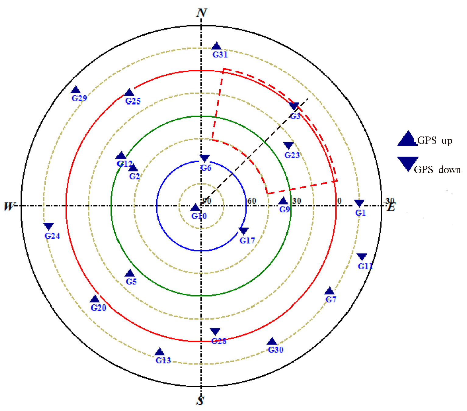
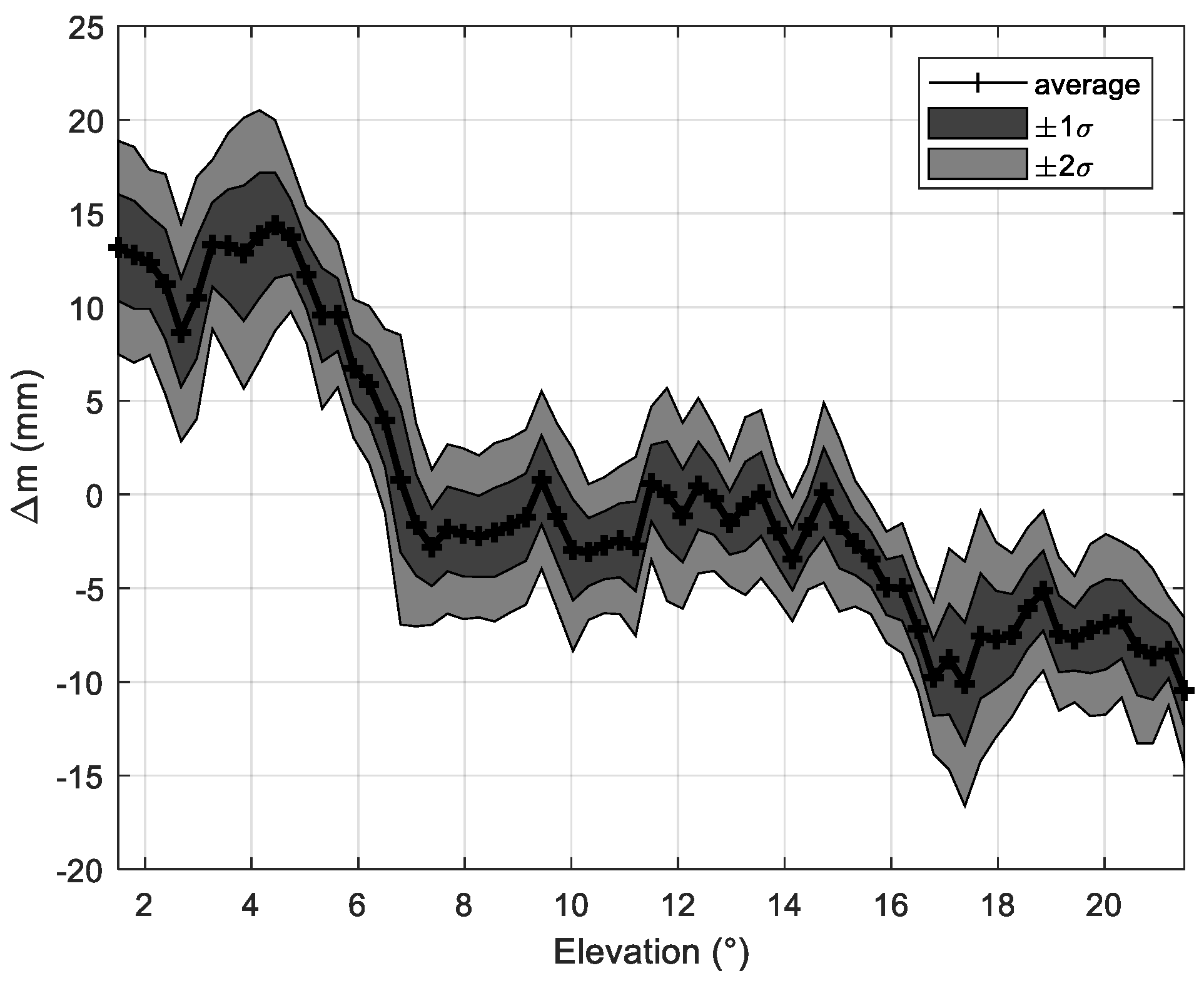
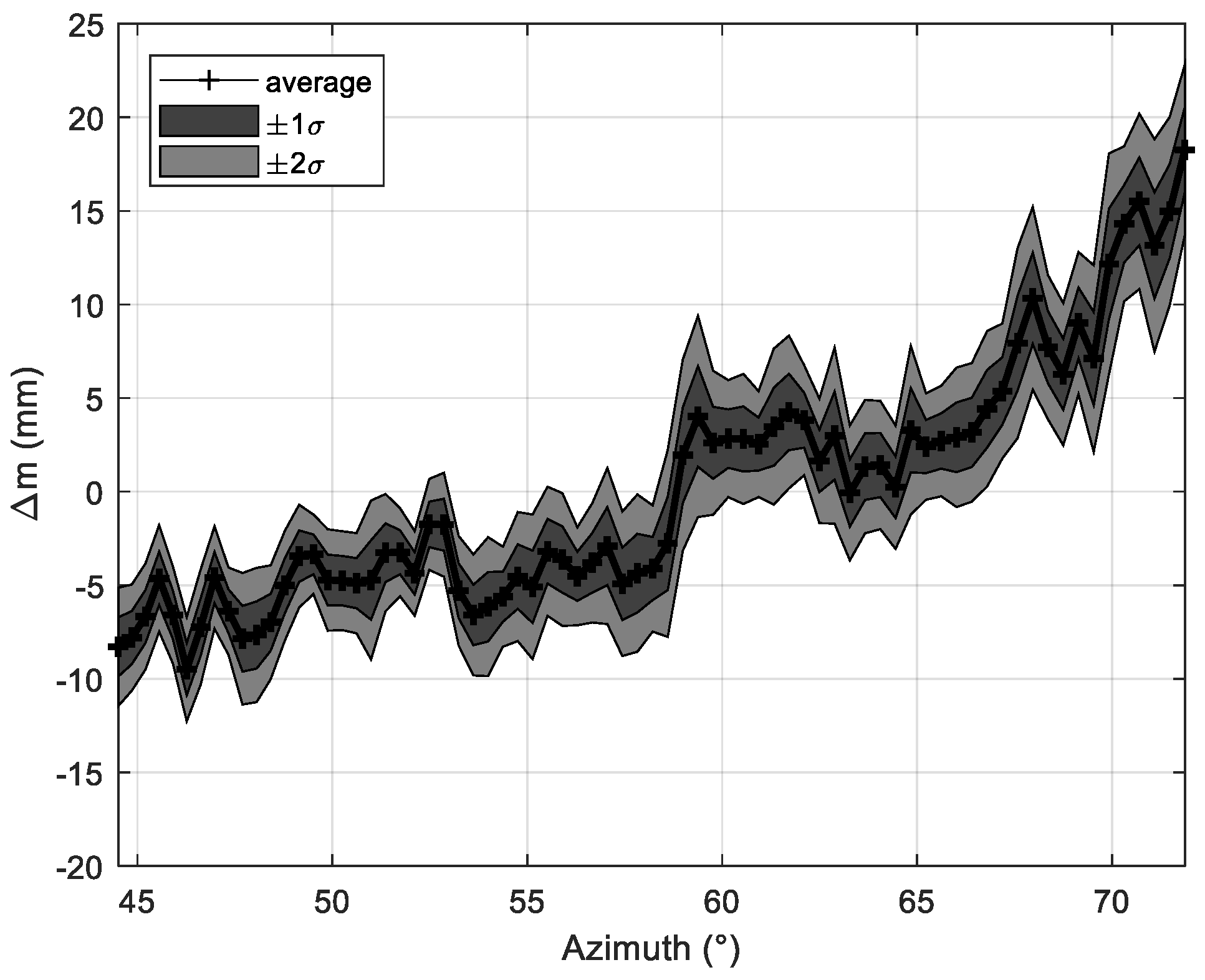
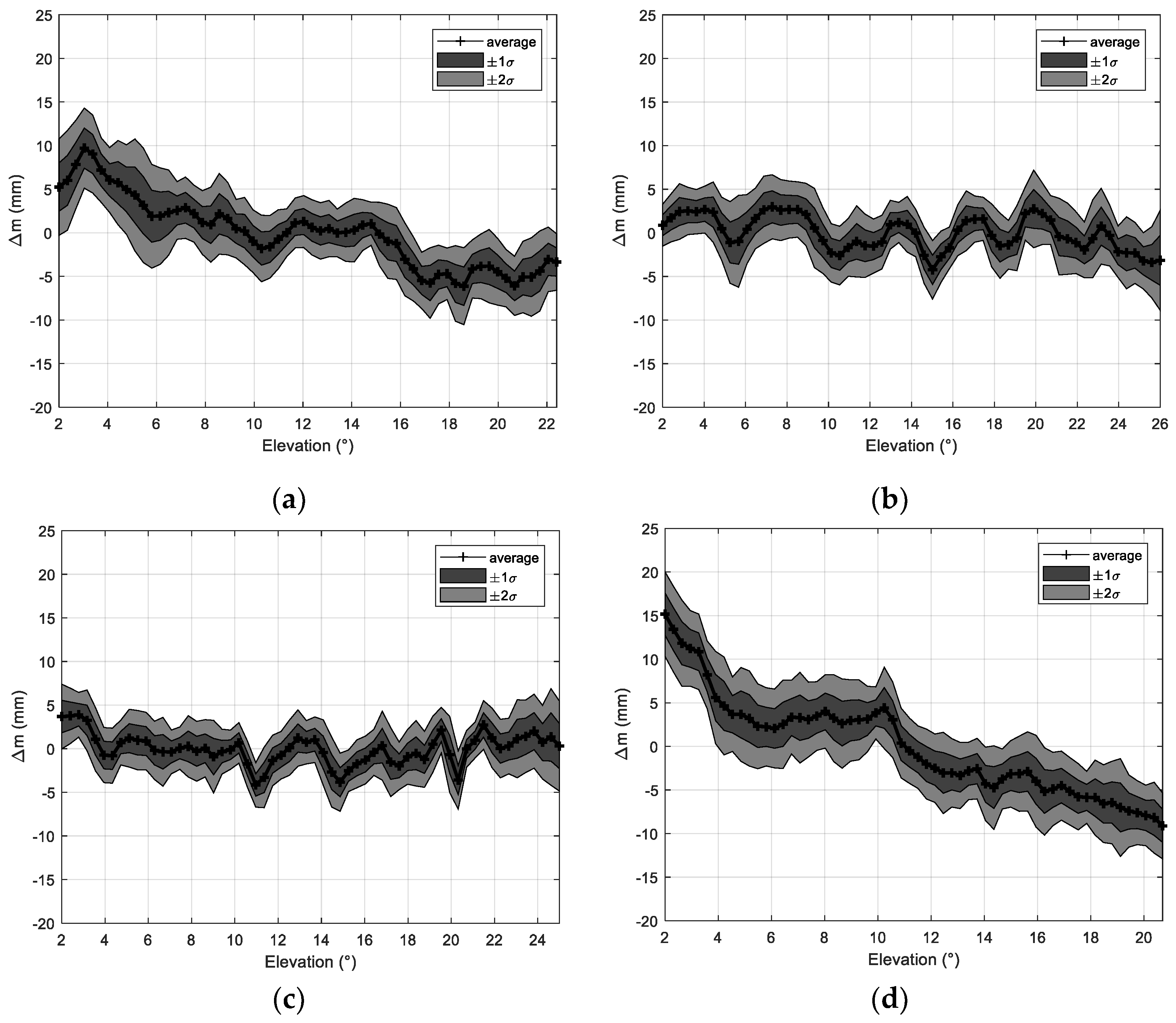
3.1. Statistical Results of G27 Satellite in 2015

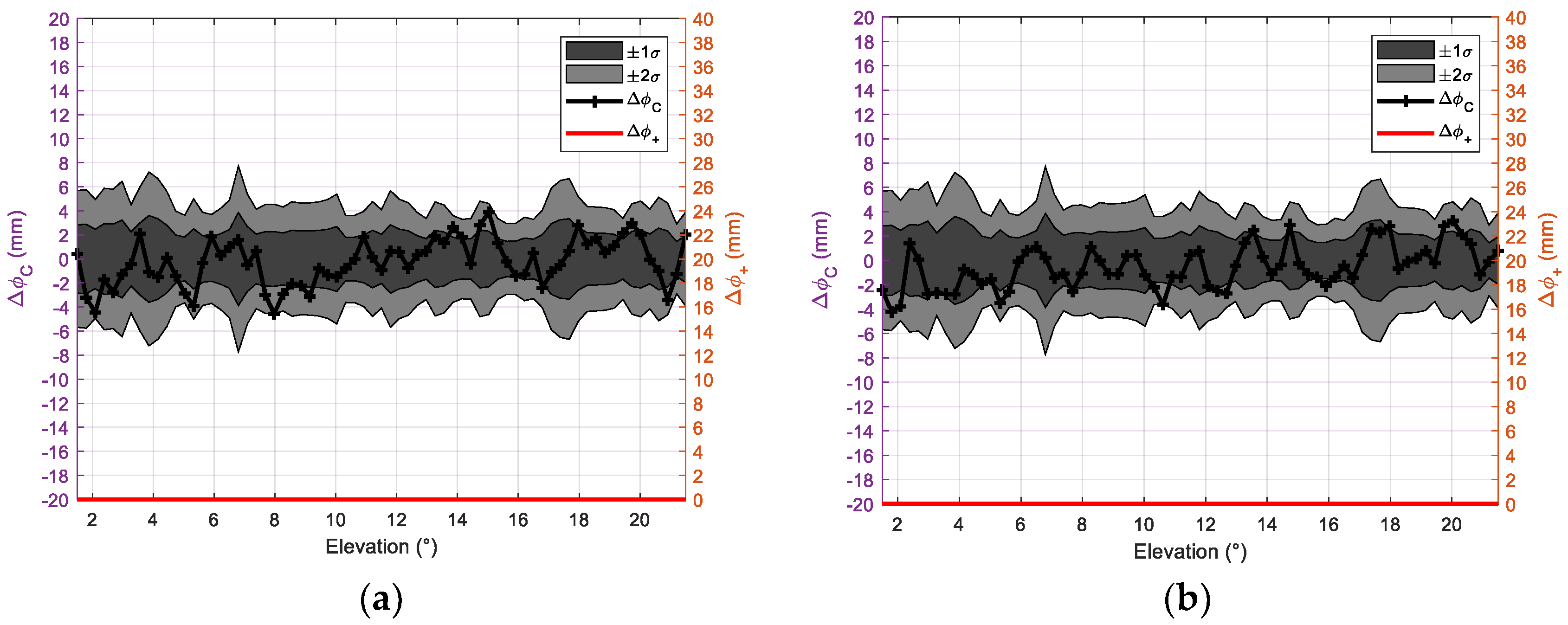
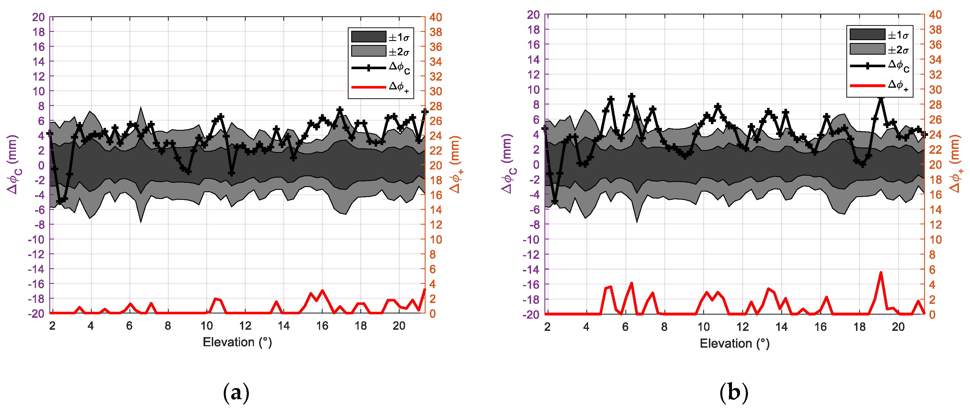
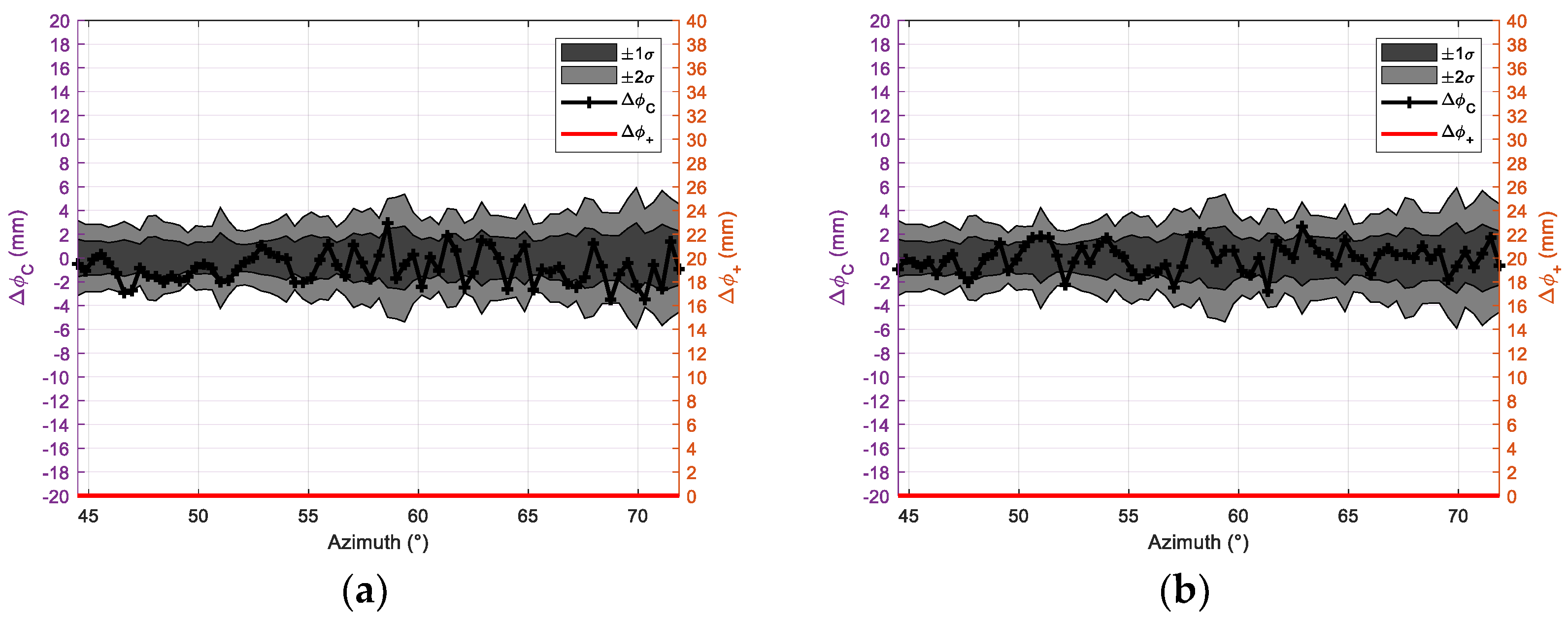
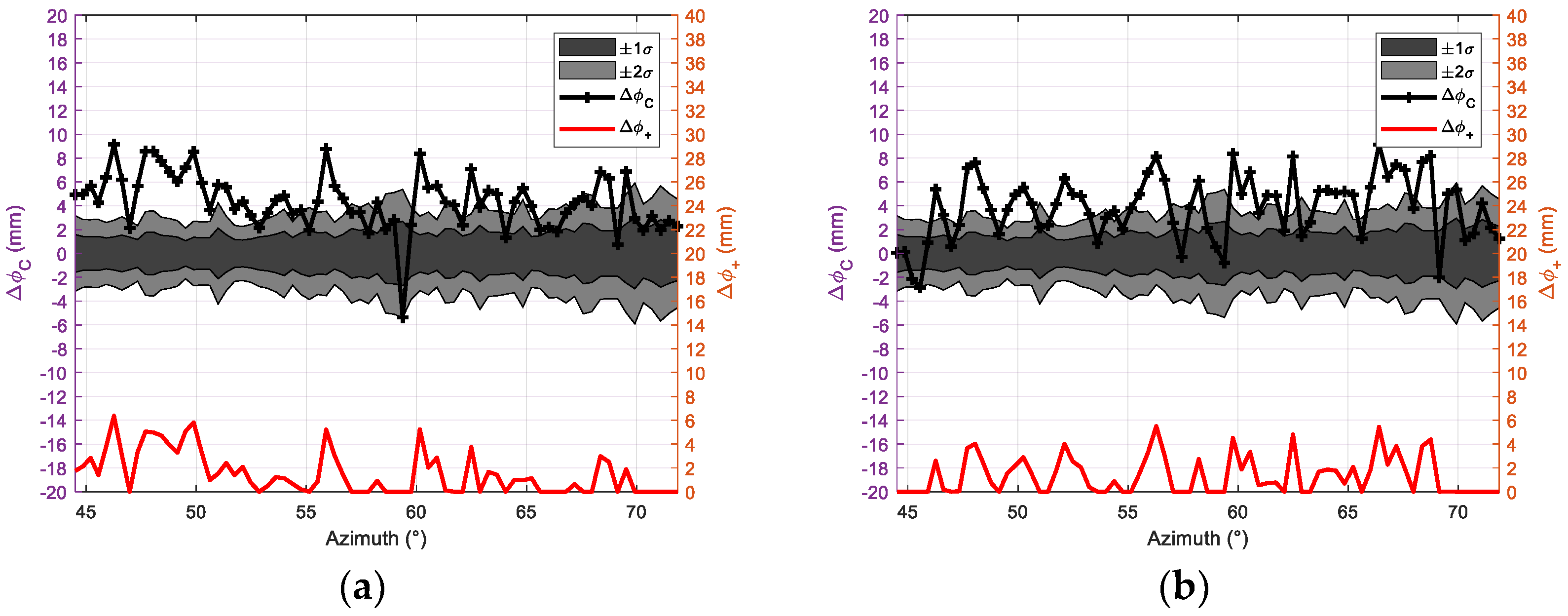
3.1.1. Phase Shift in No-Rain and Rainy Days

No-rain days are judged by the weather radar echo and the weather record. It refers to the day when the nearby stations have no record of rain during the observing period and the weather radar reflectivity of GNSS ray crossed under 1 km is 0 dBZ. Considering the availability and integrality, data from G27 is processed based on the above algorithms (Equations (4)–(8)). For our observation site, this satellite is on a descending trajectory, which makes the receiver less lock lose at the beginning of being tracked. After converting time series into elevation series, it is found that some days’ data suffers from lock lose at lower elevations. In fact, lower elevation can induce more serious phase shift [26]. Thus, in order to do statistical analysis, data with elevations ranging from 1.5° to 21.5° is selected. It is shown that usable data comes from 72 days, of which four are rainy days. In addition, daily data lasts 69 min in this elevation range. By computing the data from no-rain days, the average $\overline{\Delta m}$ and standard deviation ${\sigma }_{\Delta m}$ can be obtained, which can be seen in Figure 4.

From Figure 4, it can be seen that the average $\overline{\Delta m}$ (“black+” line) varies with the elevation. The 1 and $2{\sigma }_{\Delta m}$ thresholds are marked in dark grey and light grey, respectively. Since the carrier phase is recorded by units of length, the phase delay is obtained in mm, which is more convenient to analyze the relationship between phase delay and rain rate. The standard deviation is less than 4 mm, ranging from 1.42 mm to 3.84 mm, which indicates that the data on no-rain days has good consistency. This also implies that the multipath effect on G27 is basically stable. Furthermore, the mean of standard deviations is 2.32 mm, which is consistent with the experimental results of Padullés et al. [24].

Figure 5 presents the variations of corrected phase shift with elevation (“black+” line), whose value can be seen according to the left vertical axis. Additionally, the $\Delta {\varphi }_{+}(\beta )$ is shown by red line and its value is based on the right vertical axis. It is obvious that their $\Delta {\varphi }_C(\beta )$ are both within $\pm 2\sigma$, even their majority are in the range of $\pm 1\sigma$. Therefore, the $\Delta {\varphi }_{+}(\beta )$ are all zero, which is well matched with the fact that there is no rain during the observation period. Due to space limitation, we only take these two cases for example. But the other no-rain days’ data has the same feature.

Phase shift of two rainy days is reported in Figure 6. Since some corrected phase shifts are beyond $2\sigma$, phase shift $\Delta {\varphi }_{+}(\beta )$ are not all zero, which can be seen in red line. In addition, its maximum is more than 5 mm. By verification, it is found that there are precipitation clouds on the GPS signals’ passing area during their receiving periods (13:46–14:55 on 6 July 11:24–12:33 on 10 August). This reveals preliminarily that signals of G27 is probably affected by raindrops, resulting in creating phase shift, which still requires further research.

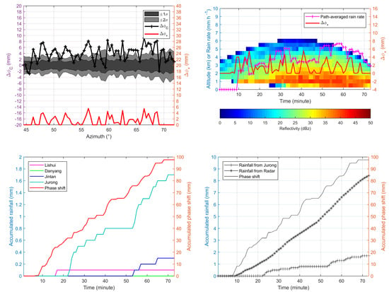
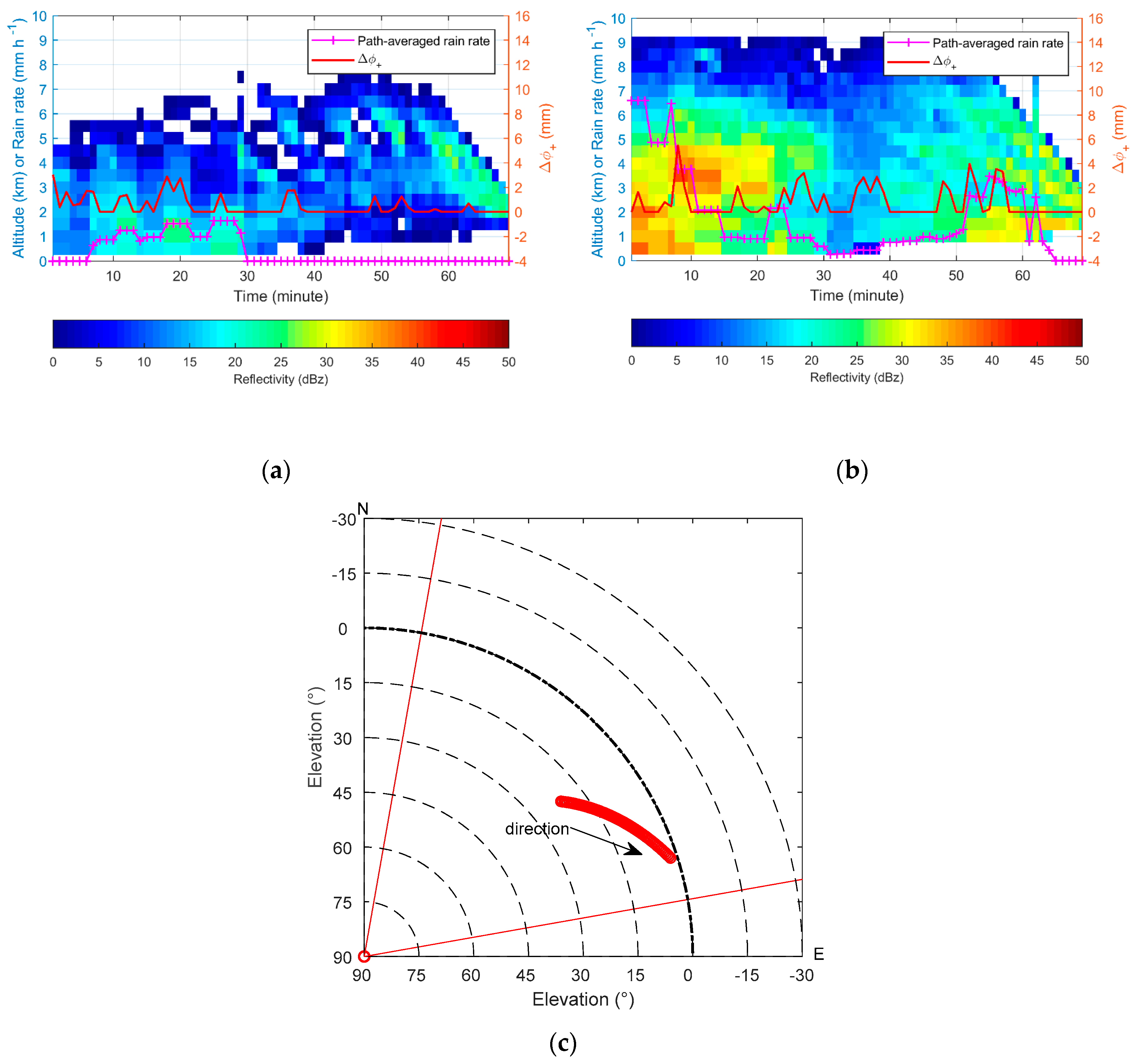
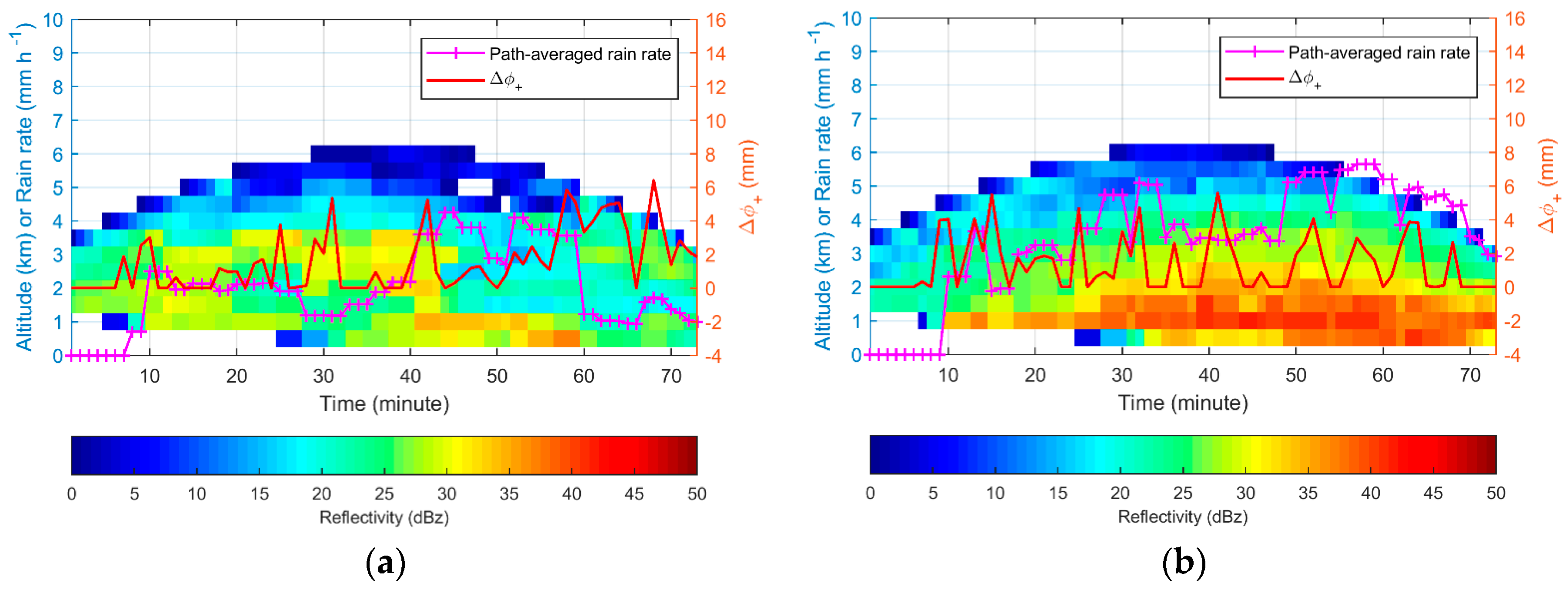
3.1.2. Comparison with Weather Radar

In order to verify the reliability of phase shift, the weather radar data in the same period is compared and analyzed.

In Figure 7a,b, each GPS ray is shown by minute and every point along the ray can be identified by its height (in km); radar reflectivity is interpolated along GPS rays, which is shown by color scale. Here, the GPS rays are assumed to be straight line propagating through rain area. The “pink+” line is the path-averaged rain rate (in mm h⁻¹) from radar reflectivity (left y axis) and phase shift $\Delta {\varphi }_{+}(\beta )$ is plotted as a red solid line with the values indicated by the right y axis. The rain rate from radar is computed using the radar reflectivity under 1 km based on a typical empirical Z-R relation ($R={\left(Z/200\right)}^{1/1.6}$) [31]. Figure 7c shows the sky view of G27 at this selected time. It has to be mentioned that once the satellite comes into the observed area (see Figure 2, enclosed by red dashed line), its signals can be tracked and received.

In the case of 6 July, it can be seen that when the phase shift is not zero, there is radar reflectivity along the GPS ray path though the radar reflectivity is weak. Moreover, the phase shift is quite obvious during 6–30 min, when the path-averaged rain rate is not zero. The case of 10 August has the similar feature. Generally, when the radar reflectivity is stronger, the maximum phase shift is larger. However, the phase shift is not obviously positive correlation with radar reflectivity. This may be due to the fact that phase shift induced by nonspherical raindrops is offseted by the difference of canting angles along GPS ray path [25]. Here, the phase shift is expected to be obtained by experiment. Fortunately, it is detected in rainy days after the above calculation.

3.1.3. Comparison with Weather Station

Figure 8a,c show the comparison between accumulated phase shift with accumulated rainfall observed from four nearby weather stations (Lishui, Danyang, Jintan and Jurong). In Figure 8a, it is obvious that only Jurong has rain during the GPS signals receiving period. Moreover, the trend of Jurong’s data is somewhat similar to that of accumulated phase shift with a correlation coefficient of 0.9709. In Figure 8c, their correlation coefficients with the data from these weather stations Lishui, Danyang, Jintan, and Jurong are 0, 0.3039, 0.9433, and 0.9114, respectively. This indicates that their accumulations have some relations, even though rain gauge is a point observation while phase shift is a linear measurement. The correlation coefficient here refer to the Person correlation coefficient, whose formula is

$$R_{XY}=\frac{{\displaystyle \sum _{i=1}^n\left(X_i-\overline{X}\right)\left(Y_i-\overline{Y}\right)}}{\sqrt{{\displaystyle \sum _{i=1}^n{\left(X_i-\overline{X}\right)}^2}}\sqrt{{\displaystyle \sum _{i=1}^n{\left(Y_i-\overline{Y}\right)}^2}}}$$

(9)

where n is the number of sample X.

It is obvious that the rain gauges variation of rain is only temporal, but for the phase the location and extension of precipitation also plays an important role. If the rain gauge is close to GPS ray and rain area, and this area is not large and sparse, the rain rate from rain gauge can represent the whole area’s rain rate. Otherwise, error is inevitable and the comparison is complex. For example, in the case of 6 July 2015, the rain area covers Jurong station during the observing period, and the GPS rays come across this rain area, getting close to Jintan station. However, there is no rain in the other three stations. Thus, Jurong station’s correlation coefficient is highest, up to 0.9433. In the case of 10 August 2015, there is no rain in Lishui station and Danyang station during the observing time. When GPS ray is close to Jintan station, it is found that the rain area covers this station from radar echoes. Therefore, Jintan station’s result is the best. When checking each GPS ray with radar precipitation echo, it can be found that the weather station, showing the best result, is basically more close to GPS ray. Therefore, the distribution of rain has an effect on this comparison analysis.

Comparisons of accumulated phase shift and accumulated rainfall obtained by different methods (retrieved from radar reflectivity and the best result of rain gauges from four weather stations) can be seen in Figure 8b,d. Though the rain rate from radar is path-averaged, which is obtained from the average of path radar reflectivity, it can also reflect the feature of rain along the GNSS ray. The correlation coefficient between accumulated phase shift and accumulated rainfall from radar is up to 0.9745 in Figure 8b and 0.9519 in Figure 8d, which are both better than the results with rain gauges. This is due to the fact that rainfall from radar is accumulation of path-averaged rain rate, which matches with GPS signals in space.

3.2. Statistical Results of G22 Satellite in 2015

3.2.1. Phase Shift in No-Rain and Rainy Days

Data from G22 is also analyzed. For the GPS antenna, this satellite’s elevation fluctuates mainly between 0° and 3°, which makes it difficult to translate its time series into elevation series. Since its azimuth varies significantly, we consider converting time series into azimuth series. Here, data with azimuth from 44° to 72° is selected. By calculation, data of 67 days are available, of which five days have rain. In addition, daily data lasts 73 min in this azimuth range. By computing no-rain days’ data, the average $\overline{\Delta m}$ and standard deviation ${\sigma }_{\Delta m}$ can be obtained, shown in Figure 9.

In Figure 9, its standard deviation ranges from 1.06 mm to 2.95 mm, with a mean of 1.78 mm, which is also quite small [24]. This reveals that the multipath effect on G22 is basically stable. Furthermore, by statistical analysis, the $\Delta {\varphi }_{+}(\beta )$ of G22 are all zero on no-rain days while not zero on rainy days.

Figure 10 displays the variations of corrected phase shift and with azimuth (“black+” line), whose value can be seen according to left vertical axis. Also, the value of $\Delta {\varphi }_{+}(\beta )$ (red line) can be seen from right vertical axis. As shown in this figure, since their $\Delta {\varphi }_C(\beta )$ are both within $\pm 2\sigma$, their $\Delta {\varphi }_{+}(\beta )$ are zero, which also coincides with the facts. Additionally, the other no-rain days’ results are similar with these two cases.

Figure 11 shows the results of two rainy days. It is obvious that their phase shift exists, whose maximum can be up to 6 mm. However, whether there are raindrops along the GPS rays still needs further research based on other data.

3.2.2. Comparison with Weather Radar

For comparison, weather radar data is also processed and analyzed. Path-averaged rain rate is also calculated from radar reflectivity. Figure 12a,b displays the results from two rainy cases, which is obtained by the same method of Figure 7a,b. In these two figures, white corresponds to “no data”. Since GPS ray does not come across cloud in this area, there is no data there. Figure 12c presents the sky view of G22 at this selected time. It is found that there are raindrops along the GPS rays, when the phase shift exists. In the case of 10 August, it is found that the radar reflectivity is quite strong. Especially, after 9 min, the path-averaged rain rate and phase shift appears almost at the same time. Furthermore, their values have some consistency. Therefore, this result still needs to be studied further.

3.2.3. Comparison with Weather Station

In Figure 13a, the tendency of accumulated rainfall from Jurong is similar with that of accumulated phase shift. Thus, their correlation coefficient is largest, up to 0.9631. From Figure 13b, the trend of accumulated rainfall from radar is well consistent with that of accumulated phase shift. Furthermore, their correlation coefficient reaches 0.9818, which is better than that with Jurong. This is also due to the fact that the path-averaged rainfall matches with GPS signals’ ray in space, while rainfall from weather station is just a point.

3.3. Statistical Results in 2016

For statistical and comparative analysis, the minimum elevation of every GPS satellite is set to 2° and the length of their data is set to one hour. Then, by calculation, it is found that the observing time of G8, G10, G11, G15, G16, G21, G26, G28, G29 is not long enough to get one-hour data, while data from other 12 GPS satellites (G1, G3, G7, G9, G12, G13, G22, G23, G24, G25, G27, G30) can be used to analyze. Their data from no-rain days is also calculated by the above processing algorithm. Some statistical results are shown in Figure 14.

From Figure 14, it is obvious that their standard deviations of the four GPS satellites’ data are small and stable, which is well consistent with the features of G22 and G27 from 2015. Besides, the other satellites’ data has the same characteristics. In order to compare, their statistical results for the no-rain days are displayed in

Table 1. Statistical results of different GPS satellites.

Satellite	Minimum Elevation (°)	Maximum Elevation (°)	Maximum Standard Deviation (mm)	Minimum Standard Deviation (mm)	Mean Standard Deviation (mm)	Number of Rainfall Cases
G1	2	22.4	3.28	1.24	1.98	4
G3	2	26.5	2.40	1.01	1.55	3
G7	2	11.2	3.63	1.08	2.0	2
G9	2	24.3	2.57	1.13	1.62	3
G12	2	26	2.87	1.15	1.73	3
G13	2	20.8	2.75	1.34	1.96	4
G22	2	25	2.77	1.03	1.63	1
G23	2	18.4	2.48	0.69	1.59	1
G24	2	23.2	2.82	1.19	1.81	1
G25	2	26.7	2.57	1.03	1.63	1
G27	2	20.7	2.81	1.49	2.17	2
G30	2	17.2	2.54	0.94	1.67	2

.

Since each satellite has its own orbit, their maximum elevations with the same minimum elevation (2°) and lasting the same time (one hour) are different, which can be seen in Table 1. Besides, obviously in Table 1, other statistics, such as maximum, minimum and mean standard deviations are reported. Statistical results on no-rain days show that the maximum standard deviation of all the satellites is 3.36 mm (G7), the minimum is low to 0.69 mm (G23), and the mean value of standard deviations from different satellites is less than 2.2 mm, with the majority within 2 mm. Besides, the samples from different satellites for statistics are all more than 80 (no-rain days). Compared with the results in Padullés et al. [24], these standard deviations here are almost the same, some even better, which demonstrates the consistency of observed data on no-rain days and the reliability of phase shift background values. This also reveals the stability of experimental equipment and feasibility of the data processing algorithm.

In Table 1, rainfall cases refer to the cases obtained by matching the phase shift of rainy day with the rain gauges. In these cases, rainfall information is detected by rain gauges. Here, some cases are shown in Figure 15.

In Figure 15, R1, R2, R3, and R4 represent the correlation coefficient between accumulated phase shift and accumulated rainfall from Lishui, Danyang, Jintan and Jurong weather stations, respectively. It can be easily seen that the tendency of each accumulated phase shift is quite similar to at least one weather stations’ rainfall data. In these cases, the optimal correlation coefficients of a case all exceed 0.96, even some up to 0.99. These results reveal the validity of the data processing algorithm and the reliability of the calculated phase shift.

4. Conclusions

This paper continues to study the feasibility of rain monitoring from polarimetric GNSS signals by performing a ground-based experiment. Firstly, based on previous theoretical research [12,25], the experiment was designed, including experimental equipment, conditions, site, and time. Especially, the key instrument, a conical horn dual-polarized GNSS antenna, was developed and used for the first time. Then, to solve some problems such as quality control, unlocking, hardware effect, phase ambiguity, multipath effect, some methods were provided successively mainly following Padullés et al. method [24], which has been applied to this ground-based experimental data. Since the multipath effect was inevitable for ground-based experiment, the method to eliminate its effect and extract phase shift proposed by Padullés et al. [24] was used. According to this data processing algorithm, experimental data in 2015 and 2016 was processed to obtain phase shift in rainy days. Finally, the phase shift was validated by weather radar and weather station data.

By analyzing data from 2 GPS satellites in 2015 and 12 GPS satellites in 2016, the results show that phase shift doesn’t exist on no-rain days. Furthermore, the standard deviations of the term ∆m induced by multipath effect are small, which is well matched with the results of Padullés et al. [24]. Fortunately, the experimental system catches some rainy cases and the rain-induced phase shift is obtained. These results verifies the feasibility of this experimental system and the data processing algorithm. They also reveal that phase shift can be observed in rainy days.

Compared with radar data, it is found that there are radar echoes along the GPS ray when phase shift occurs. In addition, by examining individual cases, the trends of accumulated phase shift and accumulated rainfall from one or more rain gauges are very similar, with some correlation coefficients up to 0.99. However, accumulated rainfall retrieved from radar reflectivity shows a more consistent trend with accumulated phase shift. This is due to the fact that rain gauge is just a point while radar can match with GPS rays in space. These comparison further demonstrates the reliability of the obtained phase shift.

Since this rain monitoring method is still in an initial phase, more research can be carried out. In this ground-based experiment, due to the effect of phase ambiguity and multipath effect, the phase shift is just relative, not absolute. Therefore, a spaceborne experiment is necessary, in which the phase ambiguity and multipath effect are easy to be solved. Our research here can provide experiment system and data processing methods for the future spaceborne experiment.

References

1. Wallace, J.M.; Hobbs, P.V. Atmospheric Science: An Introductory Survey; Academic Press: Burlington, MA, USA, 2006; pp. 1–10. [Google Scholar]
2. Baez-Villanueva, O.M.; Zambrano-Bigiarini, M.; Ribbe, L.; Nauditt, A.; Giraldo-Osorio, J.D.; Thinh, N.X. Temporal and spatial evaluation of satellite rainfall estimates over different regions in Latin-America. Atmos. Res. 2018, 213, 34–50. [Google Scholar] [CrossRef]
3. Goovaerts, P. Geostatistical approaches for incorporating elevation into the spatial interpolation of rainfall. J. Hydrol. 2000, 228, 113–129. [Google Scholar] [CrossRef]
4. Kunkel, K.E.; Andsager, K.; Easterling, D.R. Long-Term Trends in Extreme Precipitation Events over the Conterminous United States and Canada. J. Clim. 1999, 12, 2515–2527. [Google Scholar] [CrossRef] [Green Version]
5. Ricciardelli, E.; Di Paola, F.; Gentile, S.; Cersosimo, A.; Cimini, D.; Gallucci, D.; Geraldi, E.; Larosa, S.; Nilo, S.T.; Ripepi, E.; et al. Analysis of Livorno Heavy Rainfall Event: Examples of Satellite-Based Observation Techniques in Support of Numerical Weather Prediction. Remote Sens. 2018, 10, 1549. [Google Scholar] [CrossRef]
6. Gabella, M.; Speirs, P.; Hamann, U.; Germann, U.; Berne, A. Measurement of Precipitation in the Alps Using Dual-Polarization C-Band Ground-Based Radars, the GPM Spaceborne Ku-Band Radar, and Rain Gauges. Remote Sens. 2017, 9, 1147. [Google Scholar] [CrossRef]
7. Woldemeskel, F.M.; Sivakumar, B.; Sharma, A. Merging gauge and satellite rainfall with specification of associated uncertainty across Australia. J. Hydrol. 2013, 499, 167–176. [Google Scholar] [CrossRef]
8. Chandrasekar, V.; Bringi, V.N.; Balakrishnan, N.; Zrnic, D.S. Error structure of multiparameter radar and surface measurements of rainfall. Part III: Specific differential phase. J. Atoms. Ocean. Tech. 1990, 7, 621–629. [Google Scholar] [CrossRef]
9. English, M.; Kochtubajda, B.; Barlow, F.D.; Holt, A.R.; McGuinness, R. Radar measurement of rainfall by differential propagation phase: A pilot experiment. Atmos. Ocean 1991, 29, 357–380. [Google Scholar] [CrossRef] [Green Version]
10. Notaroš, B.M.; Bringi, V.N.; Kleinkort, C.; Kennedy, P.; Huang, G.-J.; Thurai, M.; Newman, A.J.; Bang, W.; Lee, G. Accurate Characterization of Winter Precipitation Using Multi-Angle Snowflake Camera, Visual Hull, Advanced Scattering Methods and Polarimetric Radar. Atmosphere 2016, 7, 81. [Google Scholar] [CrossRef]
11. Jameson, A.R. The meteorological parameterization of specific attenuation and polarization differential phase shift in rain. J. Appl. Meteorol. 1993, 32, 1741–1750. [Google Scholar] [CrossRef]
12. Yan, W.; An, H.; Fu, Y.; Han, Y.; Wang, X.; Ai, W. A method for estimating rain rate from polarimetric GNSS measurements: Preliminary analysis. Atmos. Res. 2014, 149, 70–76. [Google Scholar] [CrossRef]
13. Joyce, R.J.; Janowiak, J.E.; Arkin, P.A.; Xie, P. CMORPH: A method that produces global precipitation estimates from passive microwave and infrared data at high spatial and temporal resolution. J. Hydrometeorol. 2004, 5, 487–503. [Google Scholar] [CrossRef]
14. Huffman, G.J.; Bolvin, D.T.; Nelkin, E.J.; Wolff, D.B.; Adler, R.F.; Gu, G.; Stocker, E.F. The TRMM Multisatellite Precipitation Analysis (TMPA): Quasi-global, multiyear, combined-sensor precipitation estimates at fine scales. J. Hydrometeorol. 2007, 8, 38–55. [Google Scholar] [CrossRef]
15. Kubota, T.; Shige, S.; Hashizume, H.; Aonashi, K.; Takahashi, N.; Seto, S.; Iwanami, K. Global precipitation map using satellite-borne microwave radiometers by the GSMaP project: Production and validation. IEEE Trans. Geosci. Remote. Sens. 2007, 45, 2259–2275. [Google Scholar] [CrossRef]
16. Atlas, D.; Ulbrich, C.W. Path-and area-integrated rainfall measurement by microwave attenuation in the 1–3 cm band. J. Appl. Meteorol. 1977, 16, 1322–1331. [Google Scholar] [CrossRef]
17. Taur, R.R. Rain Depolarization Measurements on a Satellite-Earth Propagation Path at 4 GHz. IEEE Trans. Antennas Propag. 1975, 23, 854–858. [Google Scholar] [CrossRef]
18. Messer, H.; Zinevich, A.; Alpert, P. Environmental Monitoring by Wireless Communication Networks. Science 2006, 312, 713. [Google Scholar] [CrossRef]
19. Overeem, A.; Leijnse, H.; Uijlenhoet, R. Country-wide rainfall maps from cellular communication networks. Proc. Natl. Acad. Sci. USA 2013, 110, 2741–2745. [Google Scholar] [CrossRef] [Green Version]
20. Van Leth, T.C.; Overeem, A.; Leijnse, H.; Uijlenhoet, R. A measurement campaign to assess sources of error in microwave link rainfall estimation. Atmos. Meas. Tech. 2018, 11, 4645–4669. [Google Scholar] [CrossRef] [Green Version]
21. Asgarimehr, M.; Zavorotny, V.; Wickert, J.; Reich, S. Can GNSS Reflectometry Detect Precipitation Over Oceans? Geophys. Res. Lett. 2018, 45, 12–585. [Google Scholar] [CrossRef]
22. Cardellach, E.; Rius, A.; Cerezo, F. Polarimetric GNSS Radio-Occultations for Heavy Rain Detection. In Proceedings of the 2010 IEEE International Geoscience and Remote Sensing Symposium, Honolulu, HI, USA, 25–30 July 2010; pp. 3841–3844. [Google Scholar]
23. Cardellach, E.; Tomás, S.; Oliveras, S.; Padullés, R.; Rius, A.; de la Torre-Juarez, M.; Joseph Turk, F.; Ao, C.O.; Kursinski, E.R.; Schreiner, B.; et al. Sensitivity of PAZ LEO Polarimetric GNSS Radio-Occultation Experiment to Precipitation Events. IEEE Trans. Geosci. Remote Sens. 2015, 53, 190–206. [Google Scholar] [CrossRef]
24. Padullés, R.; Cardellach, E.; de la Torre Juárez, M.; Tomás, S.; Turk, F.J.; Oliveras, S.; Rius, A. Atmospheric polarimetric effects on GNSS radio occultations: The ROHP-PAZ field campaign. Atmos. Chem. Phys. 2016, 16, 635–649. [Google Scholar] [CrossRef]
25. An, H.; Yan, W.; Huang, Y.; Ai, W.; Wang, Y.; Zhao, X.; Huang, X. GNSS Measurement of Rain Rate by Polarimetric Phase Shift: Theoretical Analysis. Atmosphere 2016, 7, 101. [Google Scholar] [CrossRef]
26. Cardellach, E.; Oliveras, S.; Rius, A.; Tomás, S.; Ao, C.O.; Franklin, G.W.; de la Torre Juárez, M. Sensing heavy precipitation with GNSS polarimetric radio occultations. Geophys. Res. Lett. 2019, 46, 1024–1031. [Google Scholar] [CrossRef]
27. Sun, Y.Q.; Bai, W.H.; Liu, C.L.; Liu, Y.; Du, Q.F.; Wang, X.Y.; Yang, G.L.; Liao, M.; Yang, Z.D.; Zhang, X.X.; et al. The FengYun-3C radio occultation sounder GNOS: A review of the mission and its early results and science applications. Atmos. Meas. Tech. 2018, 11, 5797–5811. [Google Scholar] [CrossRef]
28. Blewitt, G. Carrier phase ambiguity resolution for the Global Positioning System applied to geodetic baselines up to 2000 km. J. Geophys. Res. 1989, 94, 10187–10203. [Google Scholar] [CrossRef] [Green Version]
29. Bilich, A.; Larson, K.M. Mapping the GPS multipath environment using the signal-to-noise ratio (SNR). Radio Sci. 2007, 42, RS6003. [Google Scholar] [CrossRef]
30. Yedukondalu, K.; Sarma, A.D.; Srinivas, V.S. Estimation and mitigation of GPS multipath interference using adaptive filtering. Progr. Electromagn. Res. M 2011, 21, 133–148. [Google Scholar] [CrossRef]
31. Krajewski, W.F.; Smith, J.A. On the estimation of climatological Z–R relationships. J. Appl. Meteor. 1991, 30, 1436–1445. [Google Scholar] [CrossRef]
Figure 1. Outdoor antenna section of the Global Navigation Satellite System (GNSS) dual-polarized rain detection system.
Remotesensing 11 02293 g001
Figure 2. Sky view of Global Positioning System (GPS) satellites related to the experimental site (31.6°N, 119°E) at 21:54 on 3 June 2015 and receiving area of the dual-polarized antenna (enclosed by red dashed line).
Remotesensing 11 02293 g002
Figure 3. The geographical distribution of the weather stations with respect to the observing antennas and the radar station (same with the observing antenna). The field view of the dual-polarized receiving antenna is between the two red lines in the northeast area. The radar’s detecting distances is shown by the maximum dotted circle.
Remotesensing 11 02293 g003
Figure 4. Statistical characteristics of G27 data in all no-rain days.
Remotesensing 11 02293 g004
Figure 5. Examples of phase shift from two no-rain days: (a) on 8 June 2015; (b) on 3 August 2015.
Remotesensing 11 02293 g005
Figure 6. Examples of phase shift from two rainy days: (a) on 6 July 2015; (b) on 10 August 2015.
Remotesensing 11 02293 g006
Figure 7. Examples of phase shift (red solid line with values indicated by the right y axis) from two rainy days compared with radar reflectivity (interpolated along GPS rays, whose value is shown by color scale and height is represented by left y axis) and path-averaged rain rate (“pink+” line with values indicated by the left y axis) calculated from radar reflectivity: (a) on 6 July 2015; (b) on 10 August 2015; (c) sky plot of G27 at this selected time.
Remotesensing 11 02293 g007
Figure 8. Cases of accumulated phase shift compared with accumulated rainfall observed from four weather stations and calculated from radar, respectively: (a,b) on 6 July 2015; (c,d) on 10 August 2015.
Remotesensing 11 02293 g008
Figure 9. Statistical characteristics of G22 data in all no-rain days.
Remotesensing 11 02293 g009
Figure 10. Examples of phase shift from two no-rain days: (a) on 15 June 2015; (b) on 30 August 2015.
Remotesensing 11 02293 g010
Figure 11. Examples of phase shift from two rainy days: (a) on 27 June 2015; (b) on 10 August 2015.
Remotesensing 11 02293 g011
Figure 12. Examples of phase shift from two rainy days compared with radar reflectivity and path-averaged rain rate calculated from radar reflectivity: (a) on 27 June 2015; (b) on 10 August 2015; (c) sky plot of G22 at this selected time.
Remotesensing 11 02293 g012aRemotesensing 11 02293 g012b
Figure 13. Case of accumulated phase shift on 10 August 2015 compared with accumulated rainfall observed from four weather stations and calculated from radar, respectively: (a) comparison results with data from four weather stations; (b) comparison results with data from Jurong weather station and radar.
Remotesensing 11 02293 g013
Figure 14. Statistical characteristics of four GPS satellite data in all no-rain days: (a) G1; (b) G12; (c) G22; (d) G27.
Remotesensing 11 02293 g014
Figure 15. Cases of accumulated phase shift from different GPS satellites compared with accumulated rainfall observed from four nearby weather stations: (a) G1 in Oct. 2; (b) G3 in Sep. 15; (c) G3 in Nov. 7; (d) G9 in Nov. 7; (e) G11 in Oct. 2; (f) G13 in Oct. 21; (g) G22 in Nov. 7; (h) G23 in Nov. 7; (i) G24 in Oct. 21.
Remotesensing 11 02293 g015aRemotesensing 11 02293 g015b