Determination of Global Geodetic Parameters Using Satellite Laser Ranging Measurements to Sentinel-3 Satellites

 , , , , and
Abstract
:
1. Introduction
1.1. Satellite Laser Ranging to Low Earth Orbiters
1.2. Goal and Objectives of This Study
2. Materials and Methods
2.1. Sentinel-3A/3B Mission Overview
2.2. Sentinel-3A/3B Orbits
2.3. Methodology
2.4. Solution Constraining Scenarios
2.5. The Issue of Reference Frame Differences
3. Results
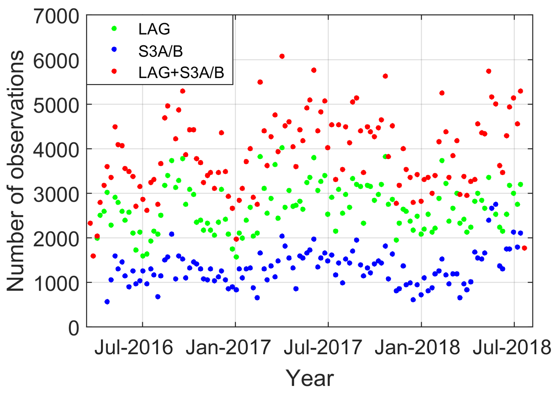
3.1. Solution Statistics
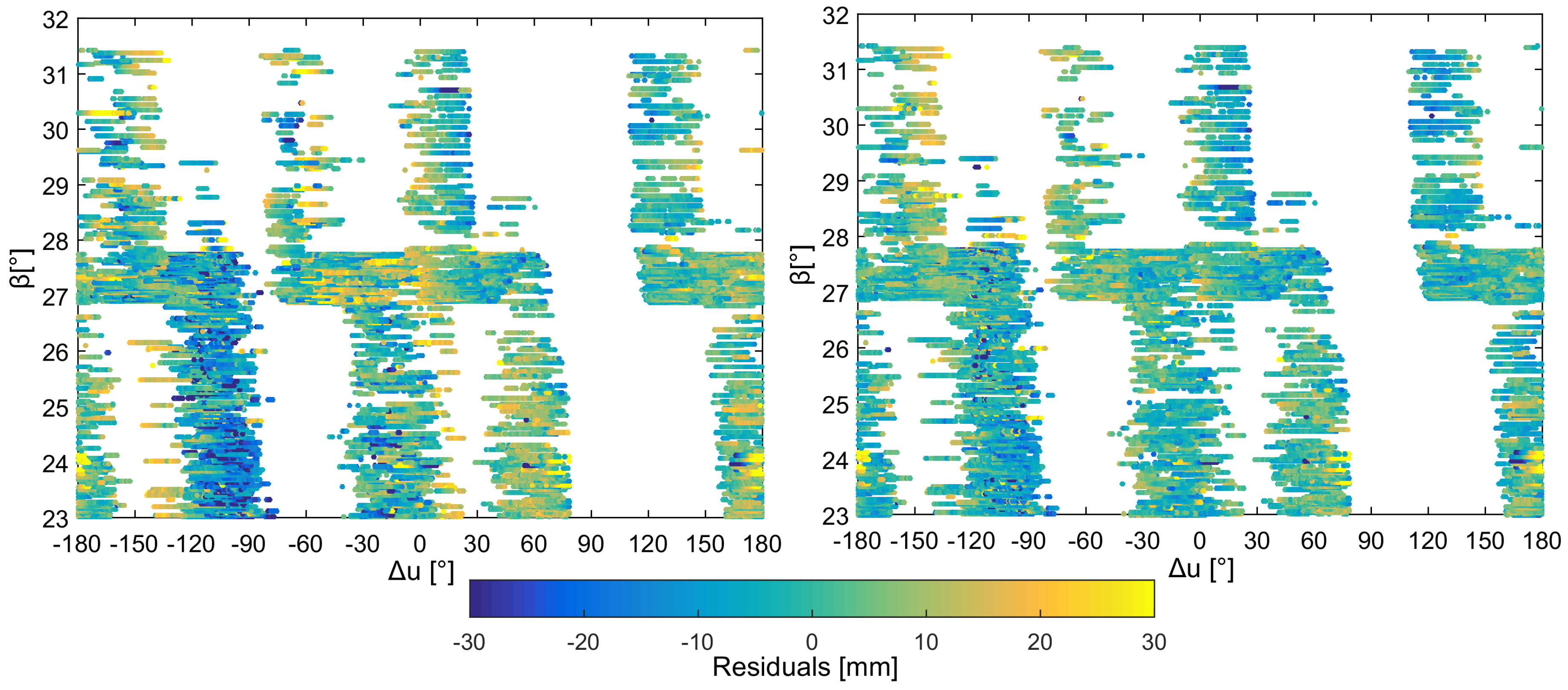
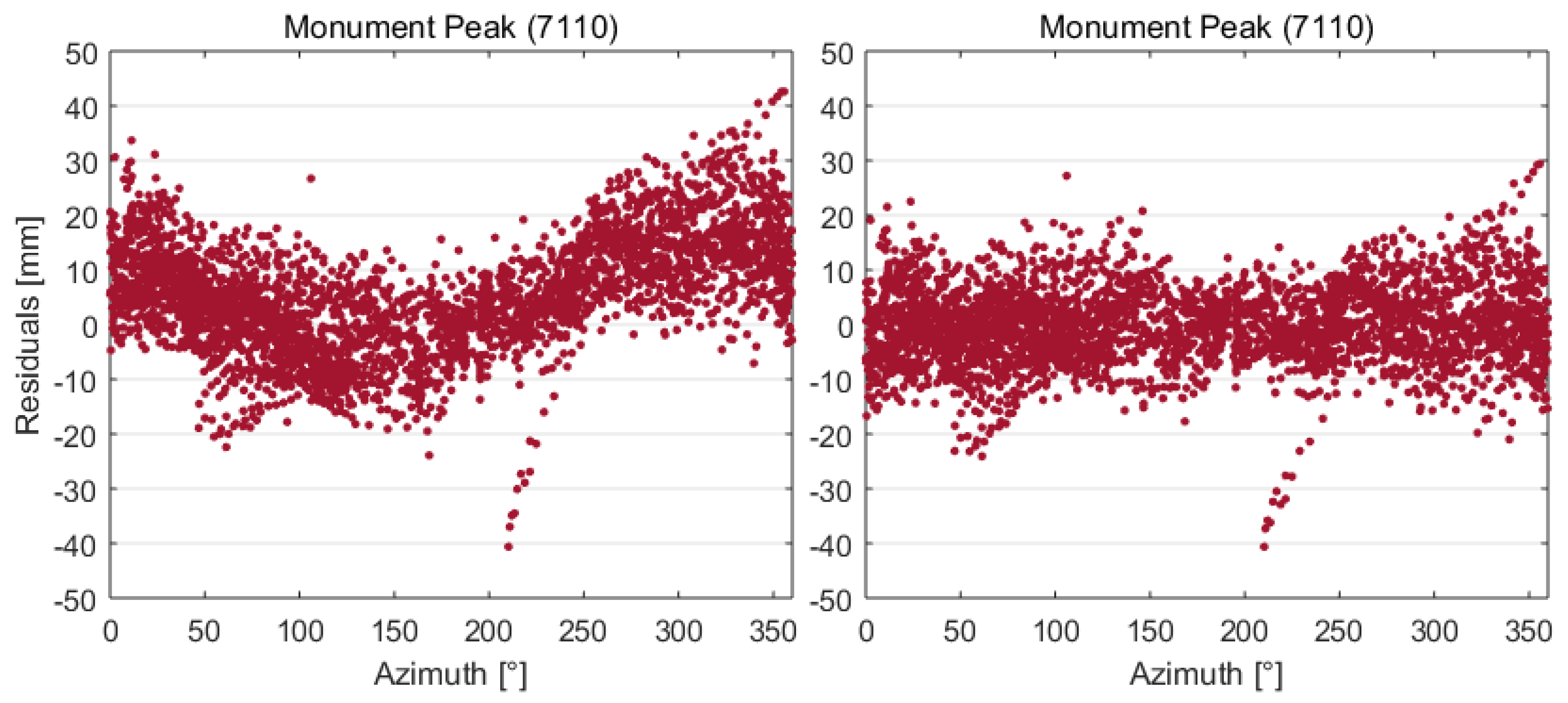
3.2. Significance of Proper Handling of Station Biases
3.3. Sentinel-3 Solution Scenario Tests
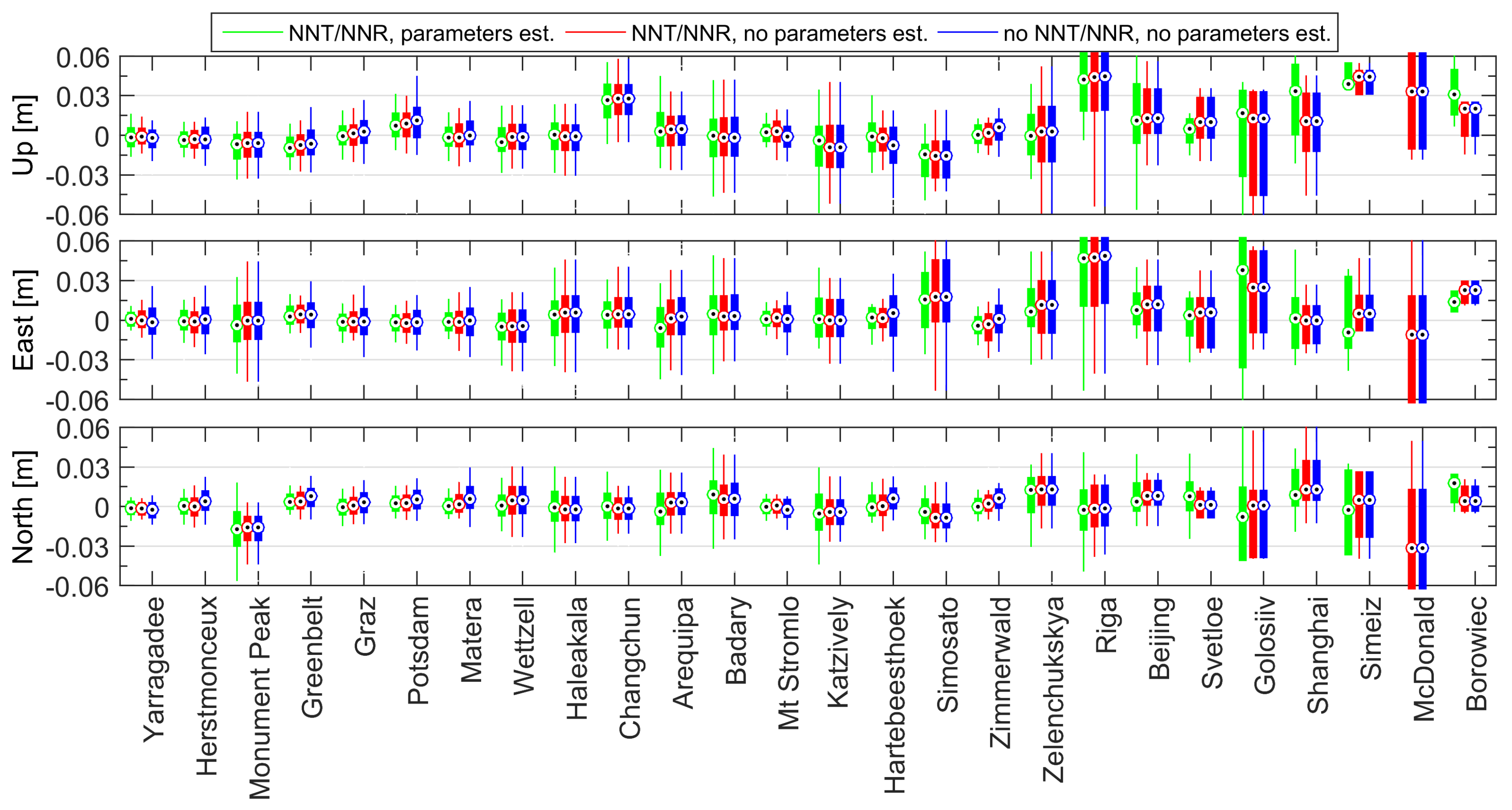
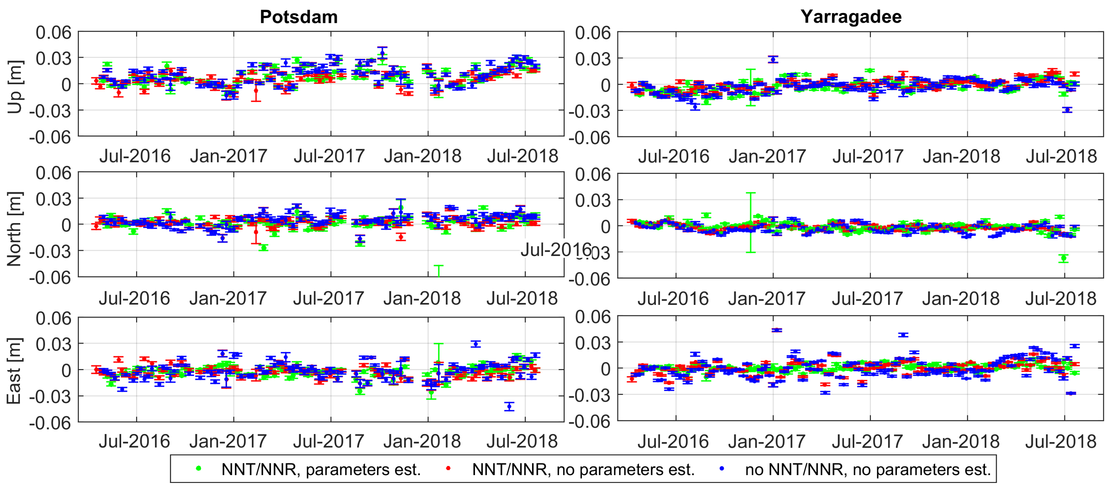
3.3.1. Station Coordinates
3.3.2. Influence of the Number of NPs on Coordinate Residual Values
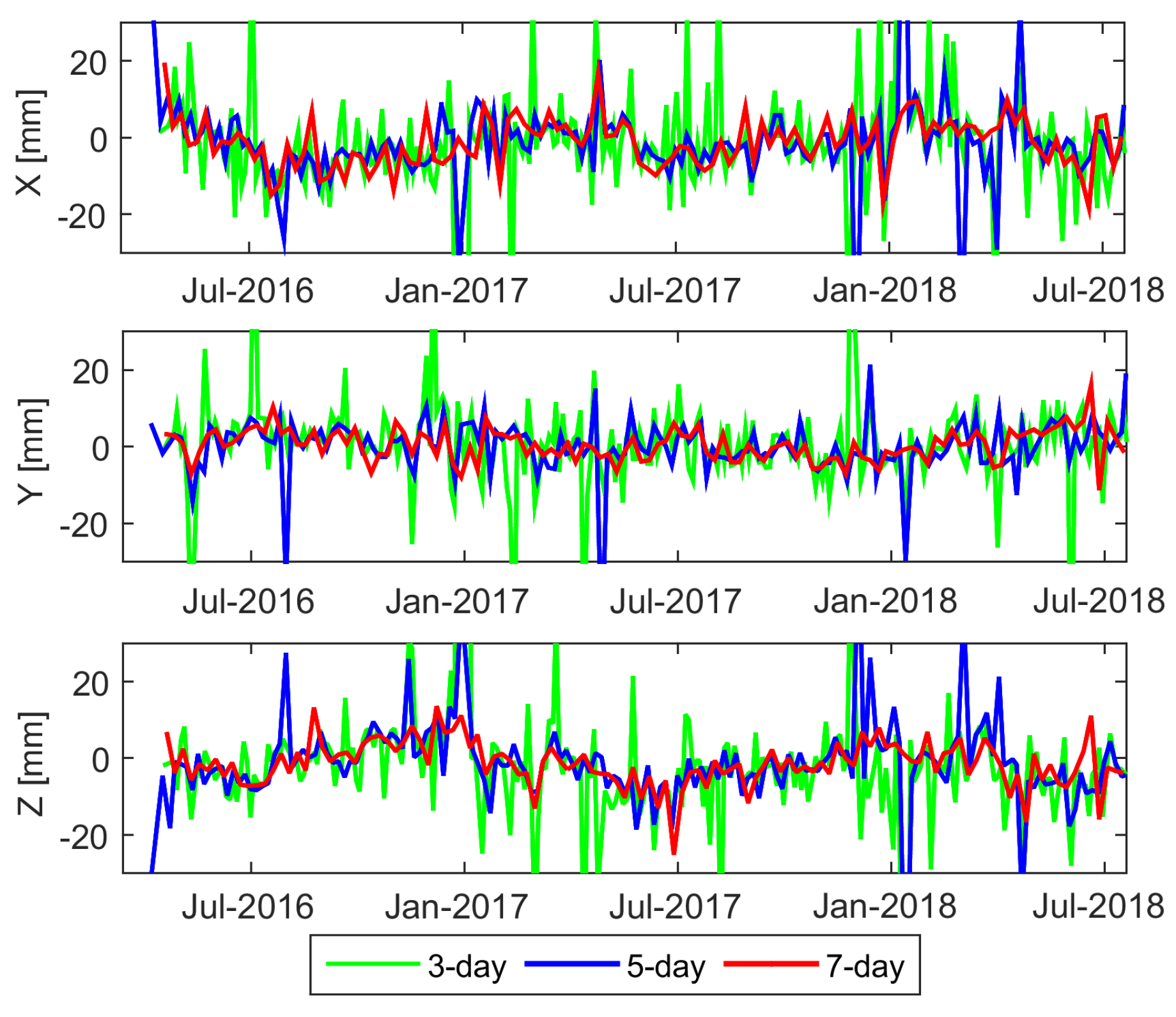
3.4. Different Numbers of Stacked 1-day Solutions
3.4.1. Station Coordinates
3.4.2. Geocenter Coordinates
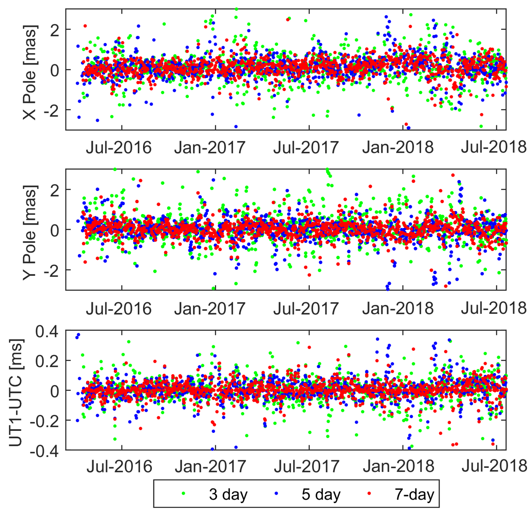
3.4.3. Earth Rotation Parameters
3.5. Combined Sentinel+LAGEOS Solutions
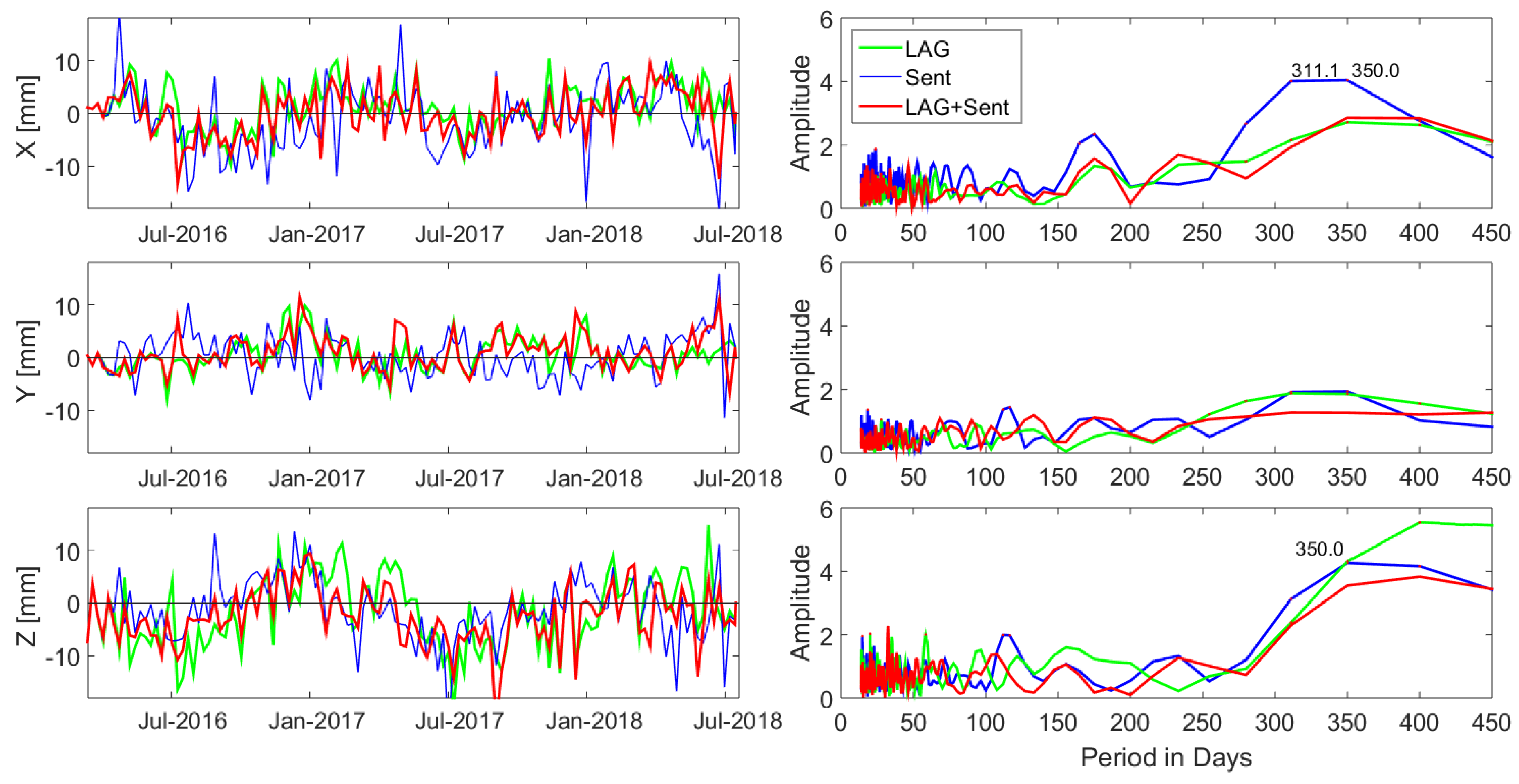
3.5.1. Geocenter from the Combined LAGEOS+Sentinel Solutions
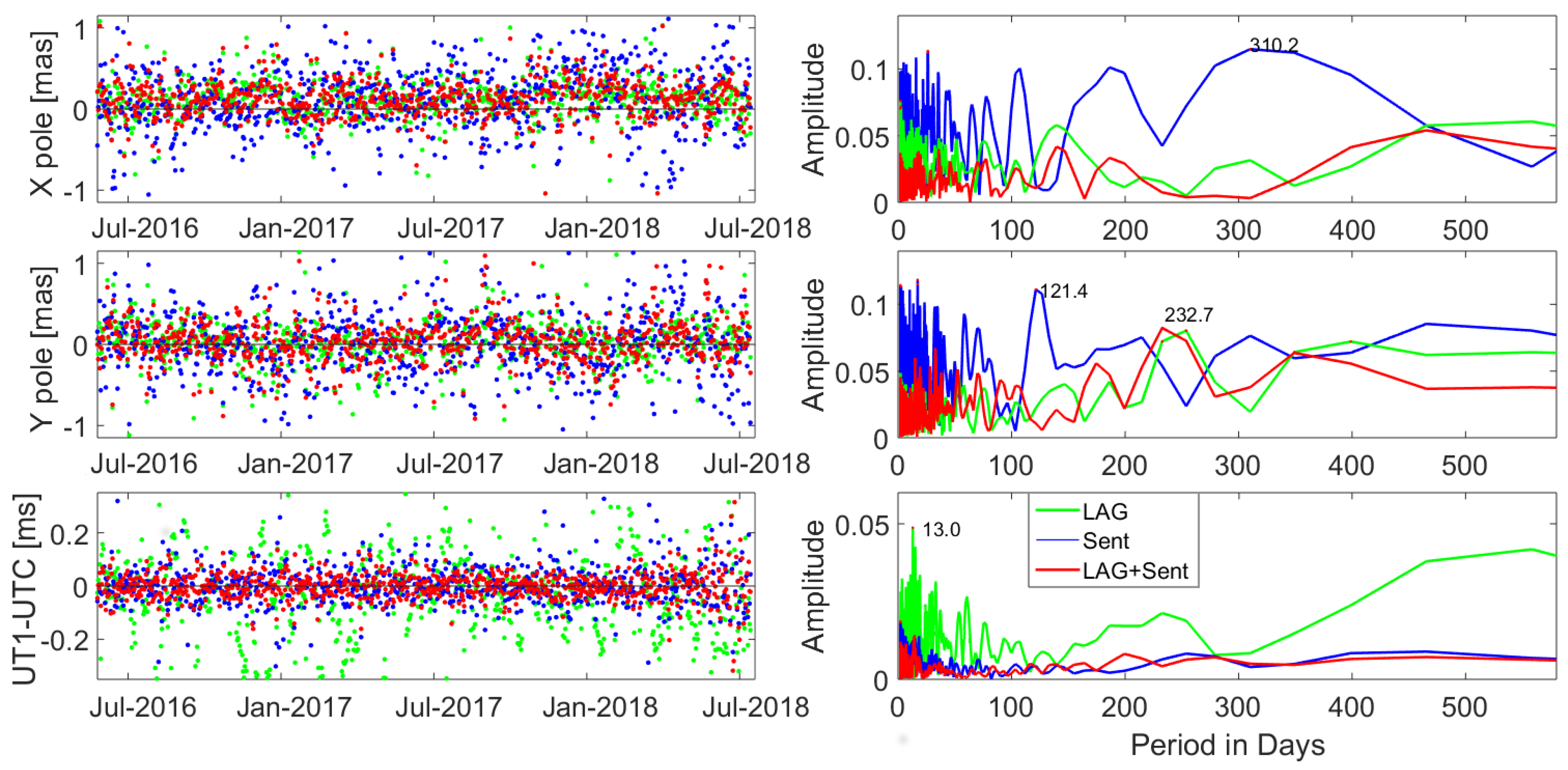
3.5.2. ERP from the Combined LAGEOS+Sentinel Solutions
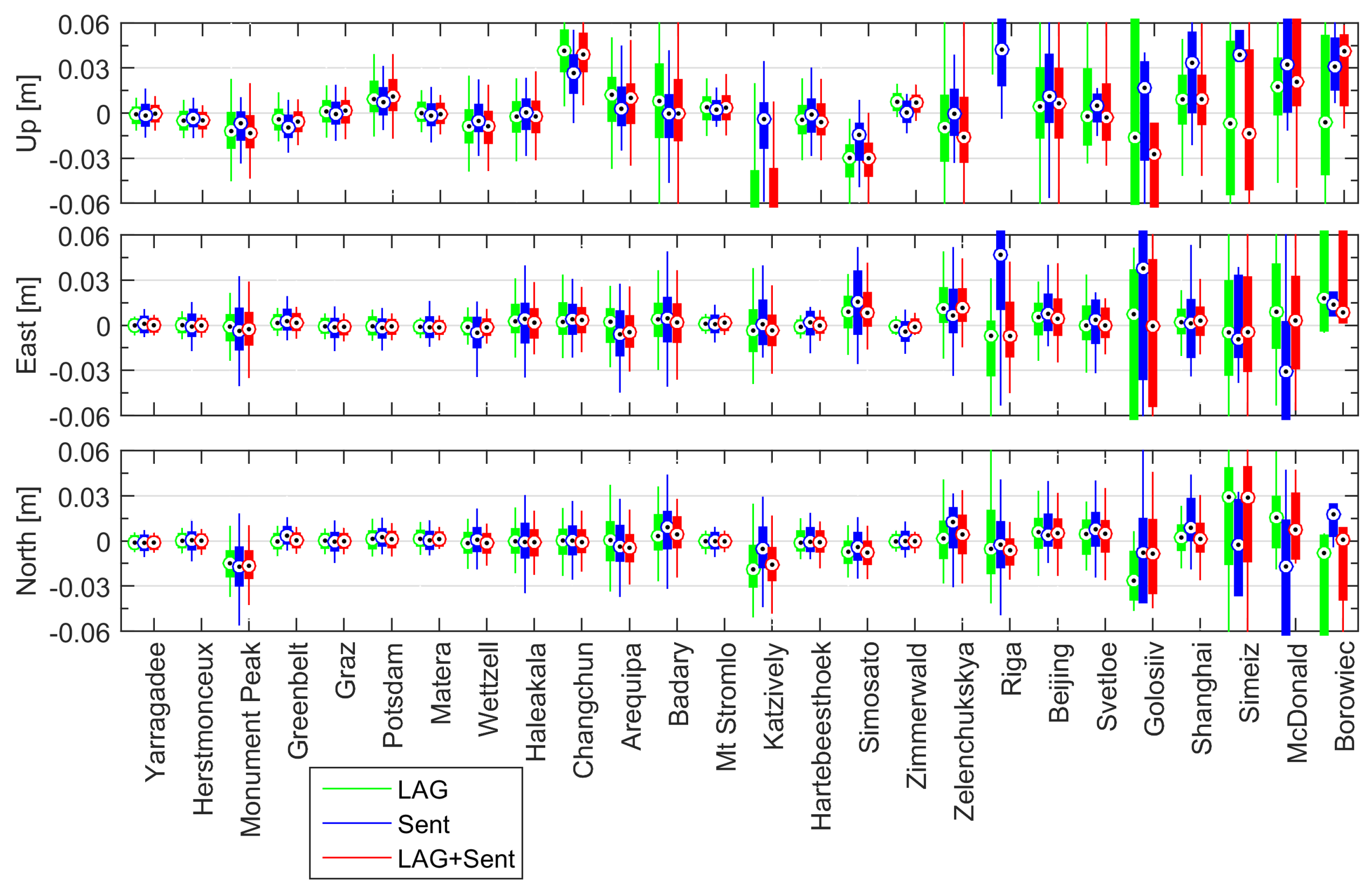
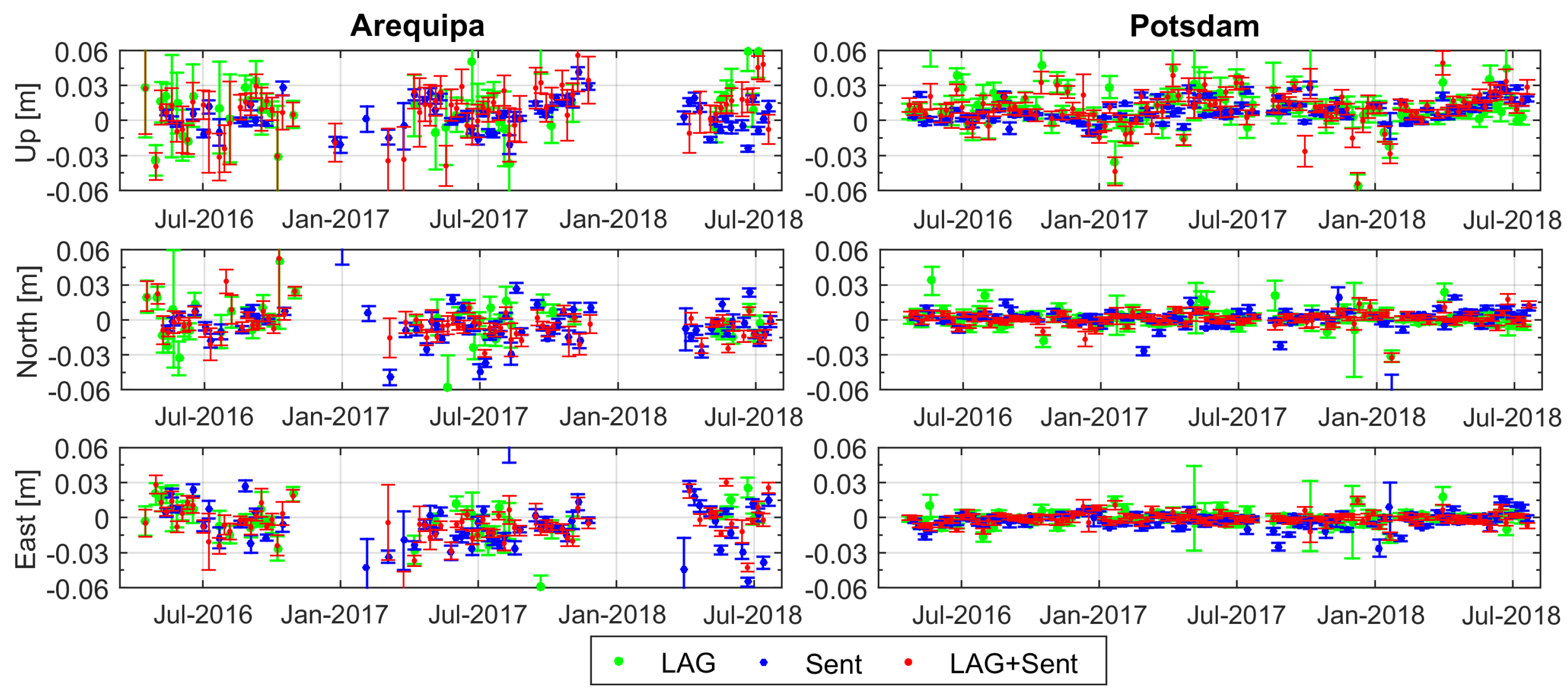
3.5.3. Station Coordinates from the Combined LAGEOS+Sentinel Solutions
4. Discussion
5. Conclusions
Author Contributions
Funding
Acknowledgments
Conflicts of Interest
Abbreviations
| S3A/B | Sentinel-3A/3B |
| SLR | Satellite Laser Ranging |
| GPS | Global Positioning System |
| ERPs | Earth Rotation Parameters |
| GNSS | Global Navigational Satellite Systems |
| LEOs | Low Earth Orbiters |
| MEO | Medium Earth Orbiters |
| DORIS | Doppler Orbitography and Radiopositioning Integrated by Satellite |
| ILRS | International Laser Ranging Service |
| POD | Precise Orbit Determination |
| AIUB | Astronomical Institute of the University of Bern |
| LRR | Laser Retroreflectors |
| CPOD | Copernicus POD Service |
| IGS | International GNSS Service |
| SLRF | Satellite Laser Ranging Frame |
| ITRF | International Terrestrial Reference Frame |
| NPs | Normal Points |
| CoM | Center of Mass |
| CoF | Center of Figure |
| NNR | No Net Rotation |
| NNT | No Net Translation |
| PPP | Precise Point Positioning |
| LAG | LAGEOS |
| IQR | Interquartile Range |
| RMS | Root Mean Square Error |
References
- Pearlman, M.; Arnold, D.; Davis, M.; Barlier, F.; Biancale, R.; Vasiliev, V.; Ciufolini, I.; Paolozzi, A.; Pavlis, E.; Sośnica, K.; et al. Laser geodetic satellites: A high accuracy scientific tool. J. Geod. 2019, 1–14. [Google Scholar] [CrossRef]
- Drinkwater, M.R.; Haagmans, R.; Muzi, D.; Popescu, A.; Floberghagen, R.; Kern, M.; Fehringer, M. The GOCE gravity mission: ESA’s first core explorer. In Proceedings of the 3rd International GOCE User Workshop, Frascati, Italy, 6–8 November 2006; pp. 1–3, ISBN 92-9092-938-3. [Google Scholar]
- Tapley, B.D.; Bettadpur, S.; Ries, J.C.; Thompson, P.F.; Watkins, M.M. GRACE Measurements of Mass Variability in the Earth System. Science 2004, 305, 503–505. [Google Scholar] [CrossRef] [PubMed] [Green Version]
- Reigber, C.; Lühr, H.; Schwintzer, P. Status of the CHAMP Mission. In Towards an Integrated Global Geodetic Observing System (IGGOS), (International Association of Geodesy Symposia, 120); Rummel, R., Drewes, H., Bosch, W., Hornik, H., Eds.; Springer: Berlin, Germany, 1998; pp. 63–65. [Google Scholar]
- Friis-Christensen, E.; Lühr, H.; Knudsen, D.; Haagmans, R. Swarm—An Earth Observation Mission investigating Geospace. Adv. Space Res. 2008, 41, 210–216. [Google Scholar] [CrossRef]
- Buckreuss, S.; Balzer, W.; Muhlbauer, P.; Werninghaus, R.; Pitz, W. The terraSAR-X satellite project. In Proceedings of the IGARSS 2003. 2003 IEEE International Geoscience and Remote Sensing Symposium. Proceedings (IEEE Cat. No.03CH37477), Toulouse, France, 21–25 July 2003; Volume 5, pp. 3096–3098. [Google Scholar] [CrossRef]
- Krieger, G.; Moreira, A.; Fiedler, H.; Hajnsek, I.; Werner, M.; Younis, M.; Zink, M. TanDEM-X: A Satellite Formation for High-Resolution SAR Interferometry. IEEE Trans. Geosci. Remote Sens. 2007, 45, 3317–3341. [Google Scholar] [CrossRef] [Green Version]
- Lambin, J.; Morrow, R.; Fu, L.L.; Willis, J.K.; Bonekamp, H.; Lillibridge, J.; Perbos, J.; Zaouche, G.; Vaze, P.; Bannoura, W.; et al. The OSTM/Jason-2 Mission. Mar. Geod. 2010, 33 (Suppl. 1), 4–25. [Google Scholar] [CrossRef]
- Donlon, C.; Berruti, B.; Buongiorno, A.; Ferreira, M.H.; Féménias, P.; Frerick, J.; Goryl, P.; Klein, U.; Laur, H.; Mavrocordatos, C.; et al. The Global Monitoring for Environment and Security (GMES) Sentinel-3 mission. Remote Sens. Environ. 2012, 120, 37–57. [Google Scholar] [CrossRef]
- Bao, L.; Gao, P.; Peng, H.; Jia, Y.; Shum, C.K.; Lin, M.; Guo, Q. First accuracy assessment of the HY-2A altimeter sea surface height observations: Cross-calibration results. Adv. Space Res. 2015, 55, 90–105. [Google Scholar] [CrossRef]
- Scharroo, R.; Bonekamp, H.; Ponsard, C.; Parisot, F.; Von Engeln, A.; Tahtadjiev, M.; De Vriendt, K.; Montagner, F. Jason continuity of services: Continuing the Jason altimeter data records as Copernicus Sentinel-6. Ocean Sci. 2016, 12, 471–479. [Google Scholar] [CrossRef]
- Arnold, D.; Montenbruck, O.; Hackel, S.; Sośnica, K. Satellite laser ranging to low Earth orbiters: Orbit and network validation. J. Geod. 2018. [Google Scholar] [CrossRef]
- Pearlman, M.; Degnan, J.; Bosworth, J. The International Laser Ranging Service. Adv. Space Res. 2002, 30, 135–143. [Google Scholar] [CrossRef]
- Hackel, S.; Gisinger, C.; Balss, U.; Wermuth, M.; Montenbruck, O. Long-Term Validation of TerraSAR-X and TanDEM-X Orbit Solutions with Laser and Radar Measurements. Remote Sens. 2018, 10. [Google Scholar] [CrossRef]
- Montenbruck, O.; Hackel, S.; van den Ijssel, J.; Arnold, D. Reduced dynamic and kinematic precise orbit determination for the Swarm mission from 4 years of GPS tracking. GPS Solut. 2018, 22, 79. [Google Scholar] [CrossRef]
- Guo, J.; Wang, Y.; Shen, Y.; Liu, X.; Sun, Y.; Kong, Q. Estimation of SLR station coordinates by means of SLR measurements to kinematic orbit of LEO satellites. Earth Planets Space 2018, 70, 201. [Google Scholar] [CrossRef] [Green Version]
- Zelensky, N.P.; Lemoine, F.G.; Ziebart, M.; Sibthorpe, A.; Beckley, B.D.; Klosko, S.M.; Chinn, D.S.; Rowlands, D.D.; Luthcke, S.B.; Pavlis, D.E.; et al. DORIS/SLR POD modeling improvements for Jason-1 and Jason-2. Adv. Space Res. 2010, 46, 1541–1558. [Google Scholar] [CrossRef]
- Couhert, A.; Mercier, F.; Moyard, J.; Biancale, R. Systematic Error Mitigation in DORIS-Derived Geocenter Motion. J. Geophys. Res. Solid Earth 2018, 123, 10142–10161. [Google Scholar] [CrossRef]
- Švehla, D.; Rothacher, M. Kinematic Orbit Determination of LEOs Based on Zero or Double-difference Algorithms Using Simulated and Real SST GPS Data. In Vistas for Geodesy in the New Millennium; Ádám, J., Schwarz, K.P., Eds.; Springer: Berlin/Heidelberg, Germany, 2002; pp. 322–328. [Google Scholar]
- Schutz, B.E.; Tapley, B.D.; Abusali, P.A.M.; Rim, H.J. Dynamic orbit determination using GPS measurements from TOPEX/POSEIDON. Geophys. Res. Lett. 1994, 21, 2179–2182. [Google Scholar] [CrossRef]
- Wu, S.C.; Yunck, T.P.; Thorton, C.L. Reduced-dynamic technique for precise orbit determination of low earth satellites. J. Guidance Control Dyn. 1991, 14, 24–30. [Google Scholar] [CrossRef]
- Hackel, S.; Montenbruck, O.; Steigenberger, P.; Balss, U.; Gisinger, C.; Eineder, M. Model improvements and validation of TerraSAR-X precise orbit determination. J. Geod. 2017, 91, 547–562. [Google Scholar] [CrossRef]
- Jäggi, A.; Hugentobler, U.; Beutler, G. Pseudo-Stochastic Orbit Modeling Techniques for Low-Earth Orbiters. J. Geod. 2006, 80, 47–60. [Google Scholar] [CrossRef] [Green Version]
- Fernández, J.; Peter, H.; Calero, E.J.; Berzosa, J.; Gallardo, L.J.; Féménias, P. Sentinel-3A: Validation of Orbit Products at the Copernicus POD Service. In International Association of Geodesy Symposia; Springer: Berlin/Heidelberg, Germany, 2019; pp. 1–8. [Google Scholar]
- Fletcher, K. Sentinel 3: ESA’s Global Land and Ocean Mission for GMES Operational Services, ESA SP-1322/3; ESA Communications: Noordwijk, The Netherlands, 2012. [Google Scholar]
- Fernández, J.; Fernández, C.; Féménias, P.; Peter, H. The Copernicus Sentinel-3 mission. In Proceedings of the ILRS Workshop 2016. pp. 1–4. Available online: https://cddis.nasa.gov/lw20/docs/2016/papers/P32-Fernandez{_}paper.pdf (accessed on 10 October 2018).
- GMV Consortium. Copernicus POD Regular Service Review Jun-Sep 2018. Tech. Rep.. 2018. Available online: https://sentinels.copernicus.eu/documents/247904/3372484/Copernicus-POD-Regular-Service-Review-Jun-Sep-2018.pdf (accessed on 10 October 2018).
- Dach, R.; Lutz, S.; Walser, P.; Fridez, P. Bernese GNSS Software Version 5.2. User Manual; University of Bern, Bern Open Publishing: Bern, Switzerland, 2015. [Google Scholar] [CrossRef]
- Dach, R.; Schaer, S.; Arnold, D.; Prange, L.; Sidorov, D.; Stebler, P.; Villiger, A.; Jaeggi, A. CODE ultra-rapid product series for the IGS; Tech. Rep.; Astronomical Institute, University of Bern: Bern, Switzerland, 2018. [Google Scholar] [CrossRef]
- Jäggi, A.; Dach, R.; Montenbruck, O.; Hugentobler, U.; Bock, H.; Beutler, G. Phase center modeling for LEO GPS receiver antennas and its impact on precise orbit determination. J. Geod. 2009, 83, 1145. [Google Scholar] [CrossRef]
- Luceri, V.; Pavlis, E.C.; Pace, B.; Kuźmicz-Cieślak, M.; König, M.; Bianco, G.; Evans, K. The ILRS Contribution to the Development of the ITRF2014. In Proceedings of the 26th IUGG General Assembly, Prague, Czech Republic, 22 June–2 July 2015. [Google Scholar]
- Bizouard, C.; Lambert, S.; Gattano, C.; Becker, O.; Richard, J.Y. The IERS EOP 14C04 solution for Earth orientation parameters consistent with ITRF 2014. J. Geod. 2018. [Google Scholar] [CrossRef]
- Sośnica, K.; Bury, G.; Zajdel, R.; Strugarek, D.; Drożdżewski, M.; Kazmierski, K. Estimating global geodetic parameters using SLR observations to Galileo, GLONASS, BeiDou, GPS, and QZSS. Earth Planets Space 2019, 71, 20. [Google Scholar] [CrossRef] [Green Version]
- Mendes, V.B.; Pavlis, E.C. High-accuracy zenith delay prediction at optical wavelengths. Geophys. Res. Lett. 2004, 31. [Google Scholar] [CrossRef] [Green Version]
- Rebischung, P.; Schmid, R. IGS14/igs14.atx: A new Framework for the IGS Products. In AGU Fall Meeting Abstracts; American Geophysical Union: San Francisco, CA, USA, 2016. [Google Scholar]
- Strugarek, D.; Sośnica, K.; Jäggi, A. Characteristics of GOCE orbits based on Satellite Laser Ranging. Adv. Space Res. 2019, 63, 417–431. [Google Scholar] [CrossRef]
- Altamimi, Z.; Rebischung, P.; Métivier, L.; Collilieux, X. ITRF2014: A new release of the International Terrestrial Reference Frame modeling nonlinear station motions. J. Geophys. Res. Solid Earth 2016, 121, 6109–6131. [Google Scholar] [CrossRef] [Green Version]
- Rodriguez-Solano, C.J.; Hugentobler, U.; Steigenberger, P.; Bloßfeld, M.; Fritsche, M. Reducing the draconitic errors in GNSS geodetic products. J. Geod. 2014, 88, 559–574. [Google Scholar] [CrossRef]
- Lutz, S.; Meindl, M.; Steigenberger, P.; Beutler, G.; Sośnica, K.; Schaer, S.; Dach, R.; Arnold, D.; Thaller, D.; Jäggi, A. Impact of the arc length on GNSS analysis results. J. Geod. 2016, 90, 365–378. [Google Scholar] [CrossRef]
- Cheng, M.; Ries, J. The unexpected signal in GRACE estimates of C20. J. Geod. 2017, 91, 897–914. [Google Scholar] [CrossRef]
- Jäggi, A.; Bock, H.; Prange, L.; Meyer, U.; Beutler, G. GPS-only gravity field recovery with GOCE, CHAMP, and GRACE. Adv. Space Res. 2011, 47, 1020–1028. [Google Scholar] [CrossRef]
- Sośnica, K.; Bury, G.; Zajdel, R. Contribution of Multi-GNSS Constellation to SLR-Derived Terrestrial Reference Frame. Geophys. Res. Lett. 2018, 45, 2339–2348. [Google Scholar] [CrossRef]
- Štěpánek, P.; Rodriguez-Solano, C.J.; Hugentobler, U.; Filler, V. Impact of orbit modeling on DORIS station position and Earth rotation estimates. Adv. Space Res. 2014, 53, 1058–1070. [Google Scholar] [CrossRef]
- Moreaux, G.; Capdeville, H.; Kuzin, S.; Otten, M.; Štěpánek, P.; Willis, P.; Ferrage, P. The International DORIS Service contribution to the 2014 realization of the International Terrestrial Reference Frame. Adv. Space Res. 2016, 58, 2479–2504. [Google Scholar] [CrossRef]
- Štěpánek, P.; Hugentobler, U.; Buday, M.; Filler, V. Estimation of the Length of Day (LOD) from DORIS observations. Adv. Space Res. 2018, 62, 370–382. [Google Scholar] [CrossRef]


| 1cSolution Scenario | Network and Parameter Constraints | ||||||
|---|---|---|---|---|---|---|---|
| NNT [m] | NNR [rad] | Scale [mm] | Geocenter crd [m] | UT1-UTC [ms] | Pole Crds [µas] | Range Bias [m] | |
| 1. NNT/NNR parameters est. | - | - | 2 | 30 | |||
| 2. NNT/NNR no parameters est. | - | ||||||
| 3. no NNT/NNR no parameters est. | - | - | - | ||||
| LAGEOS | - | - | |||||
| Sites | Solution Scenario | North | East | Up | |||
|---|---|---|---|---|---|---|---|
| Median | IQR | Median | IQR | Median | IQR | ||
| All sites | 1. NNT/NNR, all parameters est. | 0.0 | 11.7 | 0.2 | 13.4 | -0.8 | 16.3 |
| 2. NNT/NNR, no global par. est. | 0.3 | 11.5 | 1.1 | 15.2 | −0.3 | 16.9 | |
| 3. no NNT/NNR, no global par. est. | 1.7 | 14.4 | 1.4 | 19.8 | 0.0 | 18.3 | |
| Top sites | 1. NNT/NNR, all parameters est. | 0.5 | 7.8 | −0.4 | 9.1 | −1.6 | 11.9 |
| 2. NNT/NNR, no global par. est. | 1.1 | 8.5 | 0.2 | 11.4 | −0.6 | 12.3 | |
| 3. no NNT/NNR, no global par. est. | 3.2 | 11.6 | 0.4 | 16.9 | −0.7 | 13.4 | |
| Solution | X | Y | Z | |||
|---|---|---|---|---|---|---|
| Mean | RMS | Mean | RMS | Mean | RMS | |
| LAG | 1.0 | 4.3 | 0.5 | 3.1 | −1.6 | 6.8 |
| Sent | −1.0 | 6.2 | 0.3 | 4.0 | −1.2 | 6.0 |
| LAG+Sent | 0.0 | 4.5 | 0.9 | 3.4 | −2.3 | 5.9 |
| 1cSolution | X pole | Y pole | UT1-UTC | |||
|---|---|---|---|---|---|---|
| mean | RMS | mean | RMS | Mean | RMS | |
| LAG | 0.128 | 0.134 | 0.047 | 0.166 | −0.098 | 0.107 |
| Sent | 0.109 | 0.320 | 0.040 | 0.314 | −0.002 | 0.063 |
| LAG+Sent | 0.134 | 0.138 | 0.044 | 0.189 | −0.011 | 0.067 |
| 2cSolution | North | East | Up | ||||
|---|---|---|---|---|---|---|---|
| median | IQR | median | IQR | median | IQR | ||
| All sites | LAG | −0.9 | 12.7 | 0.5 | 11.1 | −0.8 | 24.6 |
| Sent | 0.0 | 11.7 | 0.2 | 13.4 | −0.8 | 16.3 | |
| LAG+Sent | −1.0 | 12.4 | 0.3 | 11.4 | −1.3 | 26.3 | |
| Top sites | LAG | −0.1 | 5.3 | 0.0 | 5.0 | −0.4 | 12.5 |
| Sent | 0.5 | 7.8 | −0.4 | 9.1 | −1.6 | 11.9 | |
| LAG+Sent | −0.2 | 5.2 | −0.1 | 5.2 | −0.7 | 12.3 | |
© 2019 by the authors. Licensee MDPI, Basel, Switzerland. This article is an open access article distributed under the terms and conditions of the Creative Commons Attribution (CC BY) license (http://creativecommons.org/licenses/by/4.0/).
Share and Cite
Strugarek, D.; Sośnica, K.; Arnold, D.; Jäggi, A.; Zajdel, R.; Bury, G.; Drożdżewski, M. Determination of Global Geodetic Parameters Using Satellite Laser Ranging Measurements to Sentinel-3 Satellites. Remote Sens. 2019, 11, 2282. https://doi.org/10.3390/rs11192282
Strugarek D, Sośnica K, Arnold D, Jäggi A, Zajdel R, Bury G, Drożdżewski M. Determination of Global Geodetic Parameters Using Satellite Laser Ranging Measurements to Sentinel-3 Satellites. Remote Sensing. 2019; 11(19):2282. https://doi.org/10.3390/rs11192282
Chicago/Turabian StyleStrugarek, Dariusz, Krzysztof Sośnica, Daniel Arnold, Adrian Jäggi, Radosław Zajdel, Grzegorz Bury, and Mateusz Drożdżewski. 2019. "Determination of Global Geodetic Parameters Using Satellite Laser Ranging Measurements to Sentinel-3 Satellites" Remote Sensing 11, no. 19: 2282. https://doi.org/10.3390/rs11192282
APA StyleStrugarek, D., Sośnica, K., Arnold, D., Jäggi, A., Zajdel, R., Bury, G., & Drożdżewski, M. (2019). Determination of Global Geodetic Parameters Using Satellite Laser Ranging Measurements to Sentinel-3 Satellites. Remote Sensing, 11(19), 2282. https://doi.org/10.3390/rs11192282