The Potential for Discriminating Microphysical Processes in Numerical Weather Forecasts Using Airborne Polarimetric Radio Occultations

Abstract

Accurate representation of cloud microphysical processes in numerical weather and climate models has proven challenging, in part because of the highly specialized instrumentation required for diagnosing errors in simulated distributions of hydrometeors. Global Navigation Satellite System (GNSS) polarimetric radio occultation (PRO) is a promising new technique that is sensitive to hydrometeors and has the potential to help address these challenges by providing microphysical observations that are relevant to larger spatial scales, especially if this type of observing system can be implemented on aircraft that can target heavy precipitation events. Two numerical experiments were run using a mesoscale model configured with two different microphysical parameterization schemes for a very intense atmospheric river (AR) event that was sampled by aircraft deploying dropsondes just before it made landfall in California, during the CalWater 2015 field campaign. The numerical experiments were used to simulate profiles of airborne polarimetric differential phase delay observations. The differential phase delay due to liquid water hydrometeors below the freezing level differed significantly in the two experiments, as well as the height of the maximum differential phase delay due to all hydrometeors combined. These results suggest that PRO observations from aircraft have the potential to contribute to validating and improving the representation of microphysical processes in numerical weather forecasts once these observations become available.

1. Introduction

Accurate representation of cloud microphysical processes has been challenging for numerical models of the atmosphere. Overcoming this challenge is critical because accumulated precipitation at the ground is dependent on microphysical processes in the atmosphere above. This problem has been approached within the framework of microphysical parameterizations, as it is not computationally feasible to explicitly resolve the complex microphysical processes that occur among hydrometeors in the atmosphere at sub-meter scales, such as collision and coalescence. Much work has been dedicated to improving microphysical parameterizations, from the inclusion of more hydrometeor species (e.g., the work by the authors of [1]), to the development of double moment schemes (e.g., the works by the authors of [2,3,4]).

The available observations of cloud microphysics used to validate numerical models and the microphysical parameterizations that they depend on have come from two main sources: (1) in situ observations and (2) radar reflectivity. In situ observations can provide detailed measurements of individual hydrometer types and size distributions. Although the sampling from in situ observations has been limited to direct aircraft and surface observation platforms, they have proven crucial in validation of microphysical parameterizations (e.g., the work by the authors of [5]) and satellite retrievals (e.g., the work by the authors of [6]), as well as in the development of forward operators for polarimetric radar (e.g., the work by the authors of [7]). Remote sensing using radar can provide observations in a much larger three dimensional volume. With conventional single polarization radar observations, what is actually measured is a combination of both the size and concentration of hydrometeors that is heavily weighted toward the largest hydrometeors (e.g., the work by the authors of [8] and references therein). Polarimetric radar observations can provide characteristics of individual hydrometeor types (e.g., the work by the authors of [9]) and drop size distributions can be derived from these observations (e.g., the work by the authors of [10]). Radar reflectivity has most commonly been used to validate numerical forecasts at single levels (e.g., the work by the authors of [11]), and for vertical profiles at a single point through time (e.g., the work by the authors of [12]). However, more recently the full vertical structure of simulated convection has been compared to radar observations [13], and dual polarization observations have been utilized to distinguish different types of hydrometeors in numerical simulations [14].

A new method for the remote sensing of precipitation has been proposed based on the detection of polarimetric effects on Global Navigation Satellite System (GNSS) radio occultation (RO) signals [15]. The GNSS RO technique is based on the principle that L-band radio navigation signals from a GNSS satellite to a receiver on a low Earth orbiting satellite or aircraft are refracted significantly when the signal is occulted by the Earth’s atmosphere [16,17]. As the GNSS satellites set or rise relative to the receiver local horizon, the signal ray path passes through successively deeper layers of the atmosphere, and a profile of refractivity with typical vertical resolution of 200–600 m can be derived from the bending angle of the ray path (see the work by the authors of [18,19] for detailed explanations of the retrieval technique). Atmospheric refractivity in the neutral atmosphere depends on moisture, temperature and pressure, with smaller effects due to liquid water, ice, and aerosols, such as dust and ash [18,20] that are usually neglected in standard retrievals for temperature and moisture profiles. Measurements from the existing constellations of spaceborne RO platforms (see the work by the authors of [21] for a review) have proven useful for observational studies of thermodynamic structure and the boundary layer (e.g., the work by the authors of [22]), the upper troposphere and lower stratosphere (e.g., the work by the authors of [23]), and routine assimilation into operational numerical weather models (e.g., the works by the authors of [24,25]).

Although the radio frequencies used in GNSS were chosen so they would be relatively insensitive to clouds and precipitation, there is a small phase delay associated with the liquid water and ice contribution to refractivity. Polarimetric RO (PRO) aims to detect the differential phase delay that hydrometeors induce in the circularly polarized electromagnetic waves using two independent and orthogonal linearly polarized antennas. The differential phase delay is mainly due to the larger amount of liquid water sampled by the horizontal component than the vertical component for oblate shaped hydrometeors, in particular, large raindrops, as is the case for weather polarimetric radars.

Although not as straightforward as polarimetric radar (e.g., with no capabilities of retrieving the 3D hydrometeor concentrations), the GNSS RO measurements have an attractive advantage in that they produce water vapor observations in the same measurement geometry and over the same spatial extent as the hydrometeor measurements, with good vertical resolution. They, thus, have the potential for testing whether the microphysical parameterization selected for a given numerical simulation is consistent with both the height dependent moisture field and the associated height distribution of hydrometeors.

The initial sensitivity studies supported the ability of the PRO technique to detect precipitation [15,26]. However, the results from a ground-based field campaign suggested that frozen particles could induce differential phase delays comparable to and larger than those predicted for large raindrops [27]. Simulations including frozen hydrometeors showed that typical ice particle concentrations can induce significant differential phase shifts if these are horizontally oriented. The complete contribution from all forms of ice is difficult to simulate, due to the limited knowledge of ice orientation in clouds. However, the results from the field campaign are consistent with significant phase delays observed well above the freezing level.

Recently, the PRO technique has been demonstrated by the Radio Occultation and Heavy Precipitation experiment on board the PAZ satellite (ROHP-PAZ), launched in May 2018 by the Institute of Space Sciences (ICE, IEEC, and CSIC) in Catalonia [28]. Overall, the first results of this previous study have shown good correlation of increased polarimetric phase delay in the presence of heavy precipitation at vertical levels consistent with the height of convective cloud tops. However, it is difficult to colocate independent observations with the ROHP-PAZ observations of sufficient density, which is required to carry out a detailed assessment of the quality of the polarimetric observations or to make a comprehensive evaluation of the polarimetric simulations. For this purpose, an airborne PRO system would be useful because it could provide targeted observations in a desired location.

Geographic sampling from spaceborne RO is relatively sparse in both time and space. To increase the sampling of a phenomenon of interest, airborne radio occultation (ARO) techniques have been developed and used in field campaigns, with promising results [29,30,31,32]. The ARO occultation profiles are concentrated within 350 km of the storm reconnaissance flight track, so many observations are available within the storm of interest. This work investigates the potential for using an aircraft platform for performing PRO measurements. An important future application of the technique is to use the information gathered about the vertical distribution of hydrometeors to validate the microphysical parameterizations used in numerical models. Here, we present a basic forward operator similar to the 2D nonlocal excess phase operator [33,34] that we modify to simulate PRO phase delays from mesoscale model output. The resulting PRO profiles are used to compare analyses and forecasts using competing microphysical parameterizations. Section 2 describes the case chosen for this study, an atmospheric river event that impacted northern California in 2015. Section 3 describes the design of the numerical experiment, the numerical forecasts of the heavy precipitation event used for the sensitivity study, and the forward operator used for the airbone PRO simulations. Section 4 describes the results, comparing the polarimetric simulations from the two numerical experiments that differ only by the microphysical parameterization scheme employed. A discussion of the applicability and limitations of the simulation results is provided in Section 5, and the conclusions and future perspectives are summarized in Section 6.

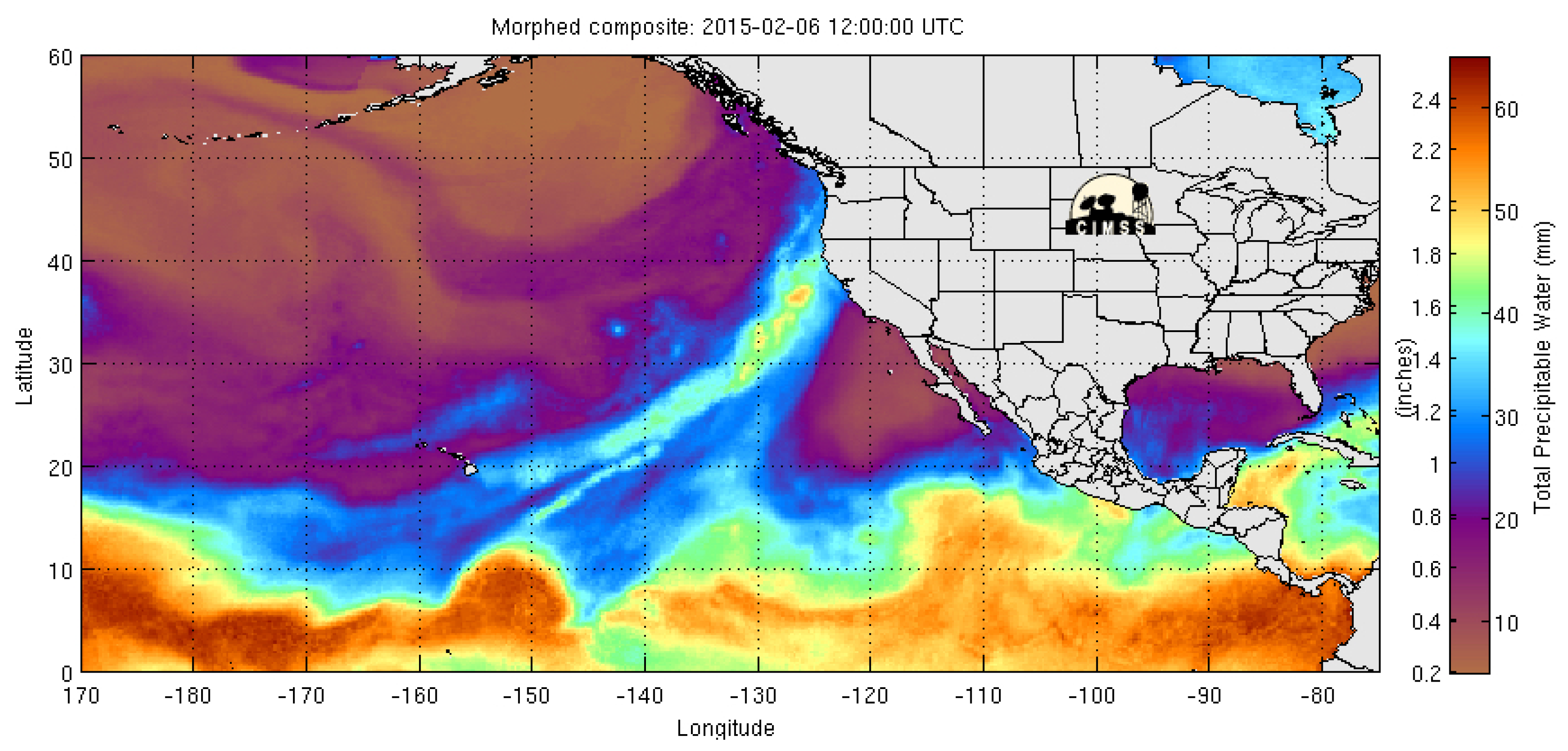
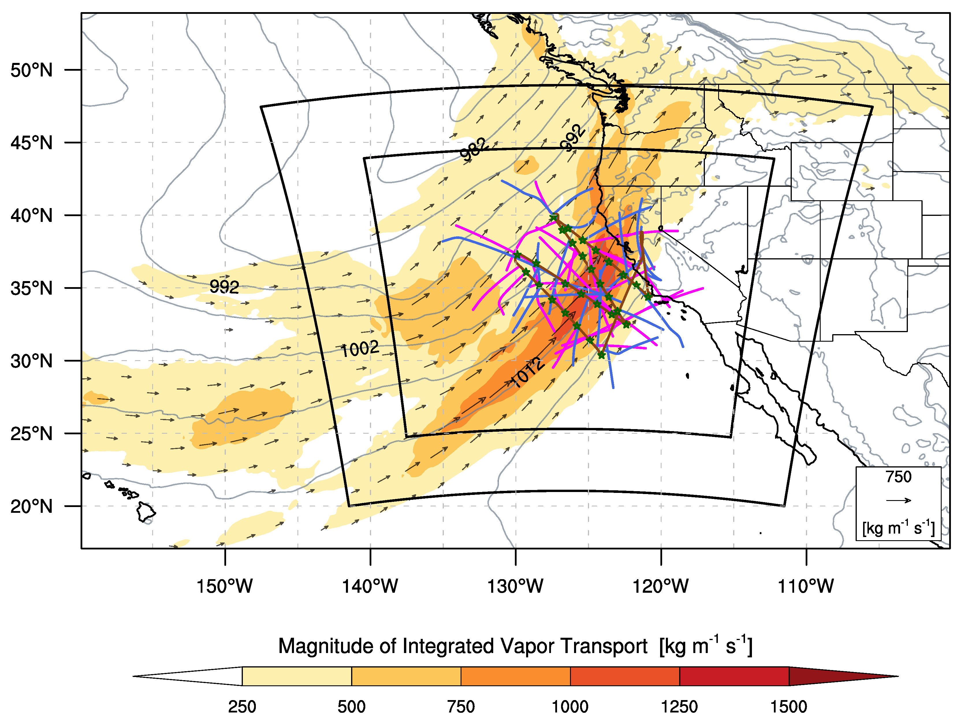
2. Atmospheric River Case Study

Atmospheric rivers (AR) are narrow, elongated plumes of moisture that are associated with a low-level jet in the warm sector of mid-latitude frontal systems [35,36]. Approximately 80–90% of the total meridional moisture flux to the mid-latitudes is provided by these features, which cover less than 10% of Earth’s circumference [37,38]. They impact predominantly the west coast of continents, including the Antarctic peninsula [38], and are exceptionally frequent in the Pacific northwestern US, Britain (e.g., the work by the authors of [39]), and Chile (e.g., the work by the authors of [40]). ARs are defined as atmospheric features having greater than 250 kg m${}^{-1}$ s${}^{-1}$ of integrated vapor transport (IVT), more than 20 mm of integrated water vapor (IWV), and having length > 2000 km and width < 1000 km [36,41], and thus have a striking signature in microwave images of integrated water vapor (i.e., Figure 1). Interaction of ARs with the coastal mountain ranges in California produces orographic precipitation that can extend for 1–5 days, in some cases causing extreme flooding [42]. For example, a series of ARs made landfall in northern California during the anomalously wet winter of 2016–2017, culminating in an intense AR that impacted the Sierra Nevada mountains in early February. The extreme precipitation led to a rapid increase in water levels on Lake Oroville, and required the use of an emergency spillway and the evacuation of nearly 200,000 people [41,43]. Flooding is recurrent in the coastal mountain ranges of northern California, and has been studied in detail in the Russian River watershed, which experienced record-breaking streamflow during the 1996 flood of Pescadero Creek [44]. The worst case to date is considered to be the historical flood of the Sacramento Valley of California in 1861–1862, which has served as the basis for extreme flooding scenarios for hazard mitigation planning [45].

AR events are an important source of precipitation, contributing 20 to 50% of the annual total in California [46]. This includes helping to build up the snowpack in Sierra Nevada, where 30–40% of the seasonal total snow water equivalent is attributed to ARs [47], providing important water resources throughout California. Whether this precipitation falls as rain or snow has a significant impact on the timing of water resource availability and distribution during the water year, and is one of the motivations for investigating microphysical processes and modeling of these storm systems [46,48]. Uplift and condensation can occur offshore within the frontal system, as well as during orographic uplift as the AR moves onshore and interacts with the topography [49,50]. Strong vertical variations associated with saturated and dry layers that are triggering and inhibiting the formation of precipitation are closely linked to the microphysical processes that determine the vertical distribution of hydrometeors as the air is uplifted.

As part of the initiative to improve mesoscale forecasting of precipitation in atmospheric river events in California, the Center for Western Weather and Water Extremes (CW3E) has developed the WestWRF regional model, oriented to the special requirements for managing water resources and the flood risk posed by extreme precipitation (https://cw3e.ucsd.edu/iwv-and-ivt-forecasts). WestWRF is an implementation of the Weather Research and Forecasting (WRF) model [51] at a spatial resolution sufficient (3 km) to represent the steep topography of the Pacific Coast of the United States (PACUS) [52]. The microphysical parameterization scheme employed in WestWRF has not yet been objectively optimized to improve the height dependent and spatially variable accumulated precipitation in the Pacific Coast and Sierra Nevada mountain ranges of California.

The 5–8 February 2015 atmospheric river event produced significant accumulated precipitation, greater than >8 cm day${}^{-1}$ for extensive regions of northern California. The atmospheric river made landfall on 6 February (Figure 1). Precipitation was measured to be greater than 20 cm at select locations in the coast ranges. The National Centers for Environmental Prediction’s (NCEP) Global Forecast System (GFS) ensembles did not pick up on the probable AR event until 30 January 2015. Precipitation was overestimated in the GFS forecasts until approximately the 60 h forecast. Considerable uncertainty in the model forecasts was due to multiple poorly defined low pressure centers and uncertainty in the trough position 3 1/2 days out, as well as uncertainty regarding the optimal microphysical and convective parameterizations for the simulations. This AR was classified retrospectively as AR 5, the highest level on the AR scale, which is considered hazardous [41].

The CalWater 2015 campaign focused on gathering observations of the structure and intensity of atmospheric rivers (ARs) over the northeastern Pacific, quantifying the moisture transport within atmospheric rivers offshore prior to landfall, and relating it to the accumulated precipitation over California [53]. Four aircraft and a research vessel participated in this multi-agency project, supported by the National Science Foundation (NSF), National Oceanic and Atmospheric Administration (NOAA), National Aeronautics and Space Administration (NASA), California Department of Water Resources (DWR), and the Department of Energy (DOE). The mission of the NOAA Gulfstream IV (G-IV) aircraft was to fly above the tropopause (~14 km) and release dropsondes to measure the moisture flux offshore in cross-sections perpendicular to the atmospheric river. The research flight used for this case study took place from 18:15 UTC 6 February to 00:45 UTC 7 February 2015 and collected dropsonde and airborne radio occultation (non-polarimetric) observations of this very intense AR while it was just offshore of northern California (Figure 2 and Figure 3). The dropsondes were released from the aircraft at regular intervals and recorded in situ observations of temperature, moisture, winds, and pressure during their descent to the surface.

Observations of accumulated precipitation are provided by the National Centers for Environmental Prediction’s (NCEP) Stage IV precipitation analysis [54]. This quantitative precipitation estimate (QPE) product is provided on a curvilinear grid (polar stereographic map projection) at ~4 km horizontal resolution over the land areas of the United States. A common rectilinear grid at a resolution of 0.05${}^{\circ }$× 0.05${}^{\circ }$ (∼4 km) was generated to ease comparison of this analysis to the numerical experiments. All precipitation fields presented herein (both model and observations) are interpolated using local area-conservative binning from their native grid to this common rectilinear grid.

3. Materials and Methods

3.1. Numerical Modeling Experiments

Two numerical experiments that differ only by their microphysical parameterization scheme are performed using the Weather Research and Forecasting (WRF) model with the Advanced Research WRF (ARW) dynamical core, version 3.7.1 [51]. The equation set used by the model is fully compressible, Euler nonhydrostatic with a terrain following hydrostatic pressure vertical coordinate. The model configuration is summarized in

Table 1. The WRF-ARW mesoscale model configuration.

Parameter	Domain 1	Domain 2
Horizontal resolution (km)	9	3
Mesh size (grid points)	360 × 350	736 × 721
Vertical layers (total #)	45	45
Time step (s)	45	15
Cumulus parameterization	Kain-Fritsch	None
Longwave radiation	RRTMG	RRTMG
Shortwave radiation	RRTMG	RRTMG
Land surface model	NOAH	NOAH
Planetary boundary layer	YSU	YSU
Surface layer	MM5 similarity	MM5 similarity

. The WRF model was configured with two nested Lambert conformal grids with horizontal resolutions of 9 km and 3 km and corresponding mesh sizes of 360 × 350 and 763 × 721 grid points, respectively (Figure 2). A two-way interactive communication occurs between the nested grids, and each grid contains 45 layers in the vertical with the finest resolution in the lowest 2 km, and with the top of the model set at 50 hPa. Computational time steps of 45 and 15 s are used on the outer and innermost grids, respectively. Physical parameterization schemes selected for use within WRF include the Kain–Fritsch convective parameterization [55], the Noah land surface model [56], the Yonsei University (YSU) planetary boundary layer scheme [57], the MM5 similarity surface layer scheme based on Monin-Obhukov similarity theory [58], and the Rapid Radiative Transfer Model for Global Climate Models (RRTMG) long wave and short wave schemes [59,60].

The initial and boundary conditions used as forcing for the numerical experiments are the European Centre for Medium-Range Weather Forecasts (ECMWF) Operational Analysis, which is available every 6 h (see http://rda.ucar.edu/datasets/ds113.0/). This product is available at much higher horizontal spatial resolution (0.141${}^{\circ }$× 0.141${}^{\circ }$ or ∼15–16 km) than other global products during this time period. A study of mesoscale forecasts initialized with various analysis products found those initialized with the ECMWF Operational Analysis to have the most accurate vertical profiles and rainfall forecasts compared to observations [61], because of better representation of temperature and moisture as compared to infrared satellite soundings.

The microphysical parameterizations used in the two numerical experiments are the WRF double moment 6-class (WDM6 [3]) and Morrison double moment [2] microphysics schemes. Both of these schemes partition condensed water into five hydrometeor species: (1) rain, (2) snow, (3) graupel, (4) cloud water droplets, and (5) cloud ice. Only a subset of these hydrometeor species have their number concentration resolved within the microphysical parameterization, and the two schemes differ on which species. Although both schemes include the number concentration of rain, the WDM6 scheme additionally includes that of cloud droplets and cloud condensation nuclei, whereas the Morrison scheme additionally includes number concentrations of the three frozen hydrometeors: snow, graupel, and cloud ice. These schemes produce variability in the characteristics of convection that is typical within mesocale simulations. Both numerical experiments were initialized at 00:00 UTC 5 February and ended at 18:00 UTC 8 February 2015.

All results presented in the following sections show standard model output variables from the WRF model with the exception of equivalent radar reflectivity, which is a derived variable calculated using the National Center for Atmospheric Research (NCAR) Command Language (NCL), and is also available from NCAR’s WRF-Python package. The NCL & WRF-Python functions (wrf_dbz and wrf.dbz, respectively) are based on the same algorithm and calculate the equivalent radar reflectivity at each grid point from the mixing ratios of rain, snow, and graupel output by the WRF model, assuming spherical hydrometeors of constant density with exponential size distributions.

3.2. Analysis of Numerical Experiments

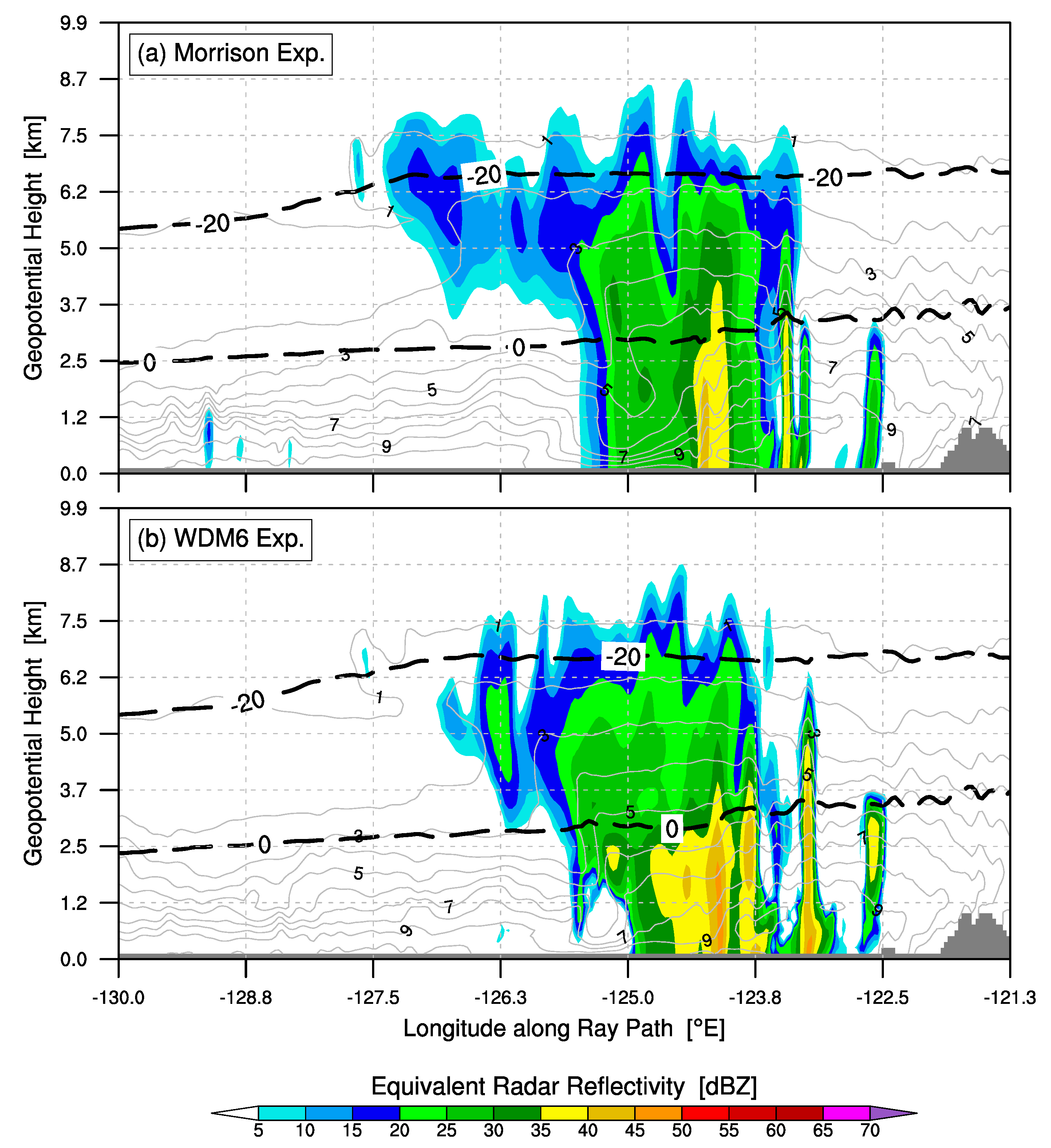
3.2.1. Equivalent Radar Reflectivity

To examine the characteristics of the simulated convection associated with the AR, the composite (i.e., columnar maximum) equivalent radar reflectivity on the innermost domain for both of the numerical experiments was calculated for 18:00 UTC 6 February 2015 (Figure 4).

This time corresponds to when the AR was making landfall in northern California and also when the rising occultation g03r from the Global Positioning System (GPS) constellation occurred. The WDM6 experiment has a larger region of composite reflectivity exceeding 30 dBZ associated with the AR compared to the Morrison experiment. These high composite reflectivity values span a larger region both along and perpendicular to the axis of the AR, from 31${}^{\circ }$N, 130${}^{\circ }$W to the northern edge of the mesoscale grid.

The geometry for all the occultations is illustrated in Figure 2 for the GPS (pink) and GLONASS (blue) satellites, with the flight track shown in brown and the dropsondes shown with green stars (see Figure 1 of the work by the authors of [29] for an illustration of the airborne RO geometry). In Figure 3, the occultations are labeled with “g” for GPS and “r” for GLONASS (the Russian equivalent of GPS), followed by the satellite number and “r” for rising and “s” for setting occultations. Figure 4 shows gray lines for the line-of-sight ray path from the aircraft to the rising GPS satellite and the corresponding pink tangent point profile. The midpoint of the longest gray line is the location of the lowest tangent point closest to the Earth surface (the end point of the pink tangent point profile line). The midpoint of the shortest gray line is the tangent point at 10 km (near the other end point of the pink tangent point profile line), and the midpoint of the middle gray line is the tangent point at 5 km. The ray paths intersect the core of the AR at approximately 38${}^{\circ }$N, as indicated in Figure 4.

To examine the vertical structure of the simulated convection, a cross section of equivalent radar reflectivity perpendicular to the axis of the atmospheric river was extracted for both numerical experiments (Figure 5). The cross section is parallel to the occultation plane (line-of-sight) of the lowest ray path of g03r. Although the WDM6 experiment has higher composite reflectivity values than the Morrison experiment across the core of the AR, approximately 123–125${}^{\circ }$W, the reflectivity values greater than 40 dBZ are concentrated below 3.5 km. In the Morrison experiment, values of reflectivity over 40 dBZ extend to a much higher vertical level, 6 km, though the maximum value is not as high as the WDM6 experiment and they occupy a much narrower band. The convection in the WDM6 experiment is shallower with large radar reflectivity returns below the freezing level at approximately 3 km, where warm rain precipitation processes dominate. The convection in the Morrison experiment extends well above the freezing level into the mixed phase region (from 0 to −20 ${}^{\circ }$C) where precipitation processes involving ice can become important.

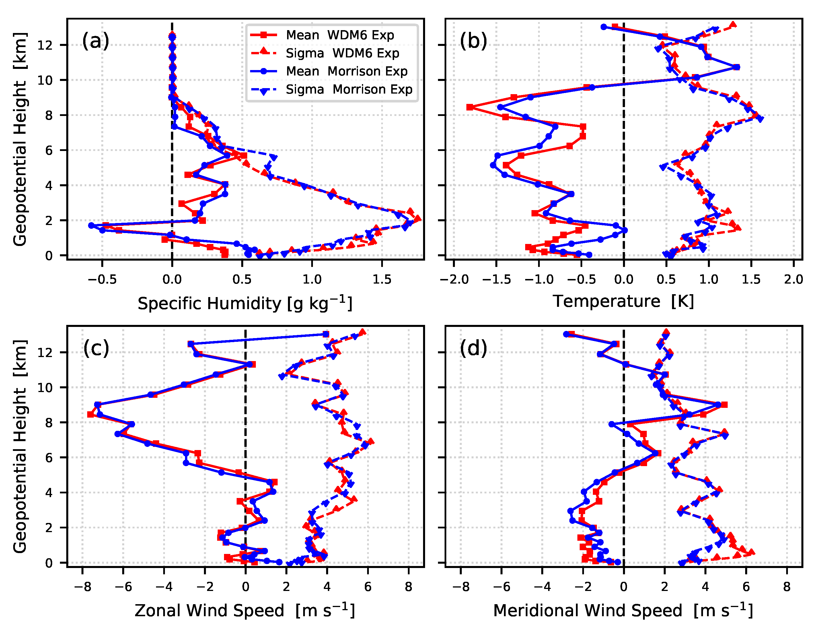
3.2.2. Comparison with Dropsonde Observations

The dropsondes released from the research flight sampled temperature, moisture, and winds in the core of the AR as it was making landfall in northern California (Figure 2 and Figure 3; green stars). These dropsonde observations are used to quantify the accuracy of the two numerical experiments in the core of the AR, by taking the mean over all dropsondes of the difference between the model value and the observations at each level in the model (Figure 6). The mean difference in specific humidity (Figure 6a) shows that both numerical experiments have 0.2–0.5 g kg${}^{-1}$ too much moisture at all levels, except at and just below 2 km in height, where both experiments are 0.5 g kg${}^{-1}$ too dry compared to the observations and the standard deviation of this difference reaches its maximum value of 1.75 g kg${}^{-1}$. This abrupt change in the profile of moisture differences may be caused by the model underestimating the depth of the moist low-level jet within the AR, with observational studies commonly identifying the top of the moisture transport at 2.25 km (e.g., the work by the authors of [62]). The largest differences between the experiments are less moisture in the lowest 1 km and more moisture at 5–8 km in the WDM6 compared to the Morrison experiment.

The mean difference in modeled minus observed temperature (Figure 6b) shows that both numerical experiments are too warm above 10 km and too cold below. The temperature difference with the observations below 10 km is 0.5–1.5 K too cold in both experiments, except at approximately 2 km in the Morrison experiment. The Morrison experiment is warmer on average than the WDM6 experiment in the lowest 2 km, and from 4 to 8 km the WDM6 is warmer than Morrison. The mean difference in winds (Figure 6c,d) shows large departures from observations in the middle to upper troposphere. The mean difference in zonal wind is much smaller between 0 and 5 km, but still up to 2 m s${}^{-1}$ in the meridional wind speed. Below 2 km, the Morrison experiment has lower wind speeds, and the WDM6 experiment has lower wind speed between 2 and 5 km.

The main difference between the thermodynamic variables in the numerical experiments is that the Morrison experiment has a warmer more moist low-level environment, along with a cooler middle troposphere than that of the WDM6 experiment. These differences between experiments lead to greater instability and an environment that is more conducive to the deeper convection in the Morrison experiment.

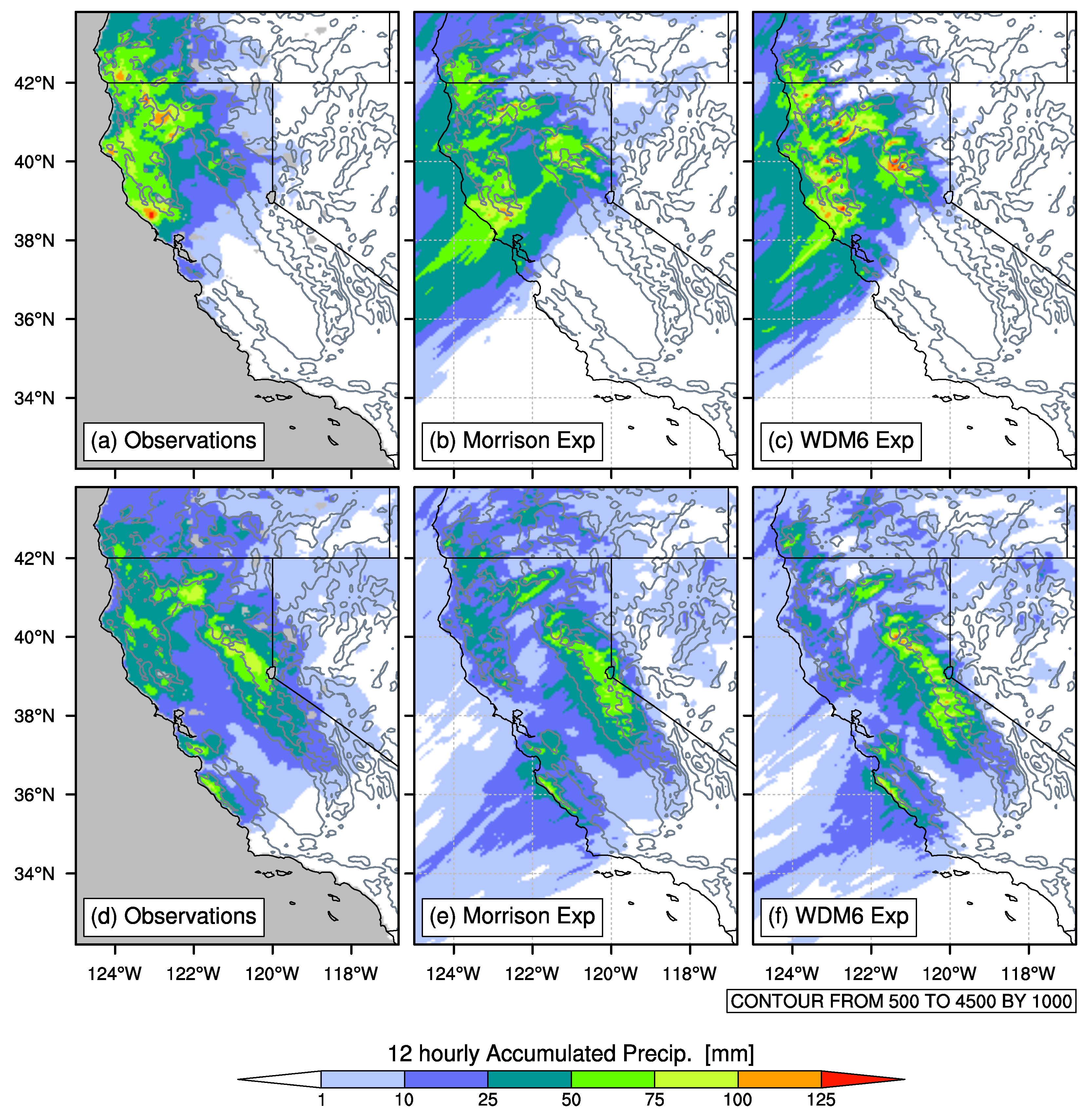
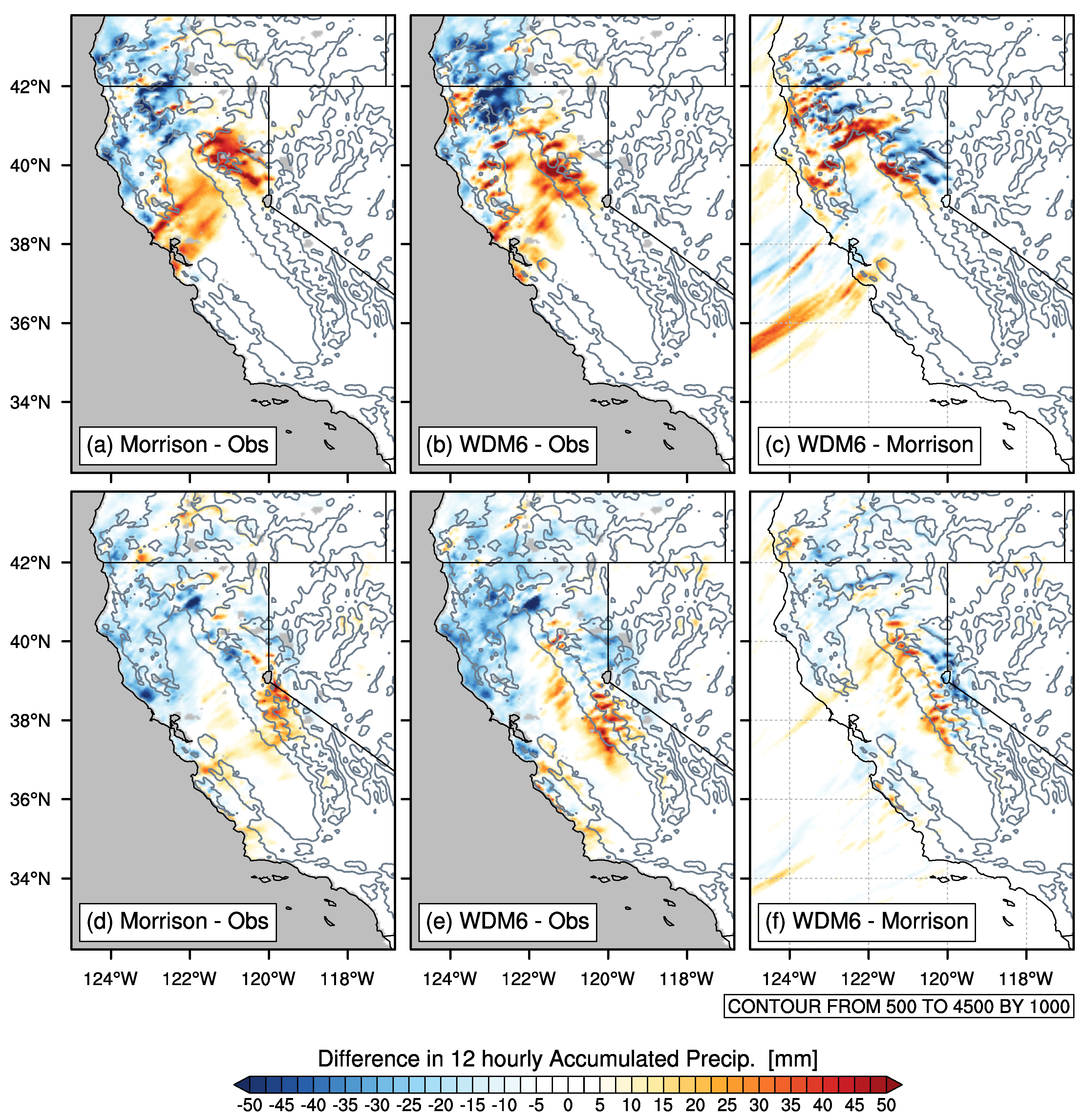
3.2.3. Accumulated Precipitation

The accumulated precipitation over the period when the atmospheric river made landfall in California is shown in Figure 7. The precipitation is divided into two 12-h accumulation periods beginning at 12:00 UTC 6 February (Figure 7a–c) and 00:00 UTC 7 February 2015 (Figure 7d–f). During the first of these 12-h periods (Figure 7a), the AR had moved into northern California and high precipitation accumulations exceeding 50 mm are found along the coastlines of southern Oregon and northern California, and in the adjacent coastal mountain ranges, with maximum exceeding 125 mm. Much less precipitation is found over the Sierra Nevada mountain range (which starts at ∼ 40${}^{\circ }$N, 121${}^{\circ }$W running southeastward to ∼ 36${}^{\circ }$N, 118${}^{\circ }$W, see terrain contours in Figure 7) in this period, with only a small part of the northernmost section of the range receiving over 25 mm of precipitation, and with little to no precipitation south of 37${}^{\circ }$N.

During the second 12-h period (Figure 7d), the AR moved further inland and the maximum in observed precipitation shifts to the Sierra Nevada range near the border with Nevada. Precipitation accumulations are lower and smaller in spatial extent during this period with maxima of less than 100 mm. The southern extent of the precipitation expands further south along the coast, where accumulations greater than 50 mm are found down to 36${}^{\circ }$N. Overall, the pattern of precipitation over the region generally follows the orography, with highest accumulations along the coast ranges, and in the higher elevations of the Sierra Nevada range. Generally lower accumulations are found between these mountain ranges in the Central Valley, though much of the northern part of the Central Valley has values above 20 mm.

The corresponding accumulated precipitation forecasts from the two numerical experiments during the first 12-h period (Figure 7b,c) shows that the model underestimates accumulation in the coast ranges and overestimates accumulation in the Sierra Nevada range. The difference in precipitation between the experiments and observations is approximately 25–50 mm over the northern Sierra Nevada as well as in the northern part of coast ranges (Figure 8a,b), and exceeds 20 mm over parts of the northern Central Valley. The clear difference in accumulated precipitation between the Morrison and WDM6 experiments is over the northern Sierra Nevada (roughly 40${}^{\circ }$N, 121${}^{\circ }$W), where the WDM6 experiment has higher accumulations on the western slopes of the Sierras, whereas the Morrison experiment has higher accumulations on the higher elevation parts of this region (Figure 8c). Other regions of difference between the numerical experiments are found in the coast ranges to the north of the San Francisco Bay area (39–40${}^{\circ }$N, 122–123${}^{\circ }$W) and also on the mountains adjacent to the northern end of the Central Valley, where the WDM6 experiment has accumulations 30–50 mm greater than that of the Morrison experiment.

The numerical experiments again follow the pattern of underestimating precipitation accumulations in the coast ranges and overestimating in the Sierra Nevada range during the second 12-h period (Figure 7e,f). Both experiments produce precipitation too far south in the Sierra Nevada, where accumulations are overpredicted between approximately 37–39${}^{\circ }$N, 121${}^{\circ }$W (Figure 8d,e). Again, the difference in accumulated precipitation between the experiments themselves is that the WDM6 experiment generates higher accumulations over the western slopes of the Sierra Nevada, whereas the Morrison experiment generates higher accumulations in the higher elevations (Figure 8f). These differences could be related to differences in hydrometeor types, with frozen particles being transported higher up slope than the heavier liquid water precipitation; however, this is dependent on the winds and other potential factors.

3.3. Polarimetric Simulation Method

The objective of this part of the work is to use the WRF mesoscale model to simulate precipitation in an atmospheric river event and to provide hydrometeor fields that can be used to estimate the range of expected values of polarimetric delay in the GNSS signals.

3.3.1. Refractivity Effects of Vapor, Liquid Water, and Ice

Usually the contribution of the neutral atmosphere to the refractive index at the L-band frequencies of GPS signals at L1 = 1.2276 and L2 = 1.57542 GHz is assumed to depend only on pressure (P), temperature (T), and water vapor pressure (e). However, refractivity includes small contributions from hydrometeors, described by relations of the more general form [18,20]:

$$N=(n-1)\times {10}^6=a_1\frac{P}{T}+a_2\frac{e}{T^2}+a_w{W}_w+a_i{W}_i$$

(1)

where $a_1=77.6$ K hPa${}^{-1}$, $a_2=3.73\times {10}^5$ K${}^2$ hPa${}^{-1}$, and $W_w$ and $W_i$ are liquid and ice content (g m${}^{-3}$), respectively, and $a_w$ and $a_i$ are $1.4$ and 0.6 (g${}^{-1}$ m${}^3$), respectively. The dispersive ionospheric effects are removed using observations on two frequencies, and the higher order ionosphere term is neglected in Equation (1). Usually the smaller effects due to liquid water, $W_w$, and ice content, $W_i$, are also neglected. However, in the case of heavy precipitation the effects of liquid water and ice on refractivity can be significant. The effect of rain rate on propagation delay, for example, is estimated to be as much as 12 mm km${}^{-1}$ of path through the rain region and $3\%$ of the total refractive delay [20]. These authors also estimated the delay for other hydrometeors including hail and snow.

3.3.2. Simulation of Polarimetric Effects

The investigation of the effects of liquid water was advanced further by also considering polarization of the GNSS-RO signals for detecting the presence of large raindrops from forward scattering effects [15,63]. Assuming large nonspherical raindrops, the proposed sensitivity to heavy precipitation predicts a differential delay for H/V polarized GPS signals. Given some assumptions on the drop size distribution, the polarimetric phase shift accumulated along the ray path L is of the form

$$\Delta {\varphi }^{atm}={\int }_L{K}_{dp}\left(l\right)dl\mathrm{and}$$

(2)

$$K_{dp}=\frac{{\lambda }^2}{2\pi }\int \mathcal{R}\{f_h\left(D\right)-f_v\left(D\right)\}N\left(D\right)dD$$

(3)

where D is the particle diameter; $f_h\left(D\right)$ and $f_v\left(D\right)$ are the forward scattering amplitudes of the horizontally and vertically polarized signals, respectively; $N\left(D\right)$ is the drop size distribution; and $K_{dp}\left(l\right)$ is the specific differential phase (in mm-shift/km-rain). The real parts of the scattering amplitudes $f_h\left(D\right)$ and $f_v\left(D\right)$ in Equation (3) are numerically calculated via the T-matrix method [64] and strongly depend on the aspect ratio of the particle shape model of [65], r,

$$r={\left(1.0048+5.7\times {10}^{-4}D-2.628\times {10}^{-2}{D}^2+3.682\times {10}^{-3}{D}^3-1.677\times {10}^{-4}{D}^4\right)}^{-1}.$$

(4)

The rain rate $RR$ for the drop size distribution $N\left(D\right)$ is given by

$$RR=0.6\pi {10}^{-3}\int 3.778N\left(D\right)D^{3.67}dD$$

Then, $K_{dp}$ at each point along the observation ray path is tabulated along with the rain rate. This is used in the numerical integration along the ray path in Equation (2), to forward model the total polarimetric delay.

This approach has been applied in studies using remotely sensed rain rate data to infer a dropsize distribution and estimate the magnitude of the polarimetric delay [15,66]. They simulated the differential effect of the two orientations for raindrops compared to spherical particles integrated over different path lengths, to show that the polarimetric delays were above the detectable limit (3 mm in the absolute accuracy of the GPS phase measurement) for rain rates above 3 mm/h and path lengths greater than 25 km. This simulation method was used for planning the polarimetric RO mission for the ROHP-PAZ satellite [15,27] and in the preliminary analysis of the mission results [28].

3.3.3. Raytracing Simulation of Polarimetric Delay

We calculate the ray paths for the expected ARO signals from the positions of the NOAA G-IV aircraft and the GNSS satellite positions on that day, given by the precise orbit files of the International GNSS Service Multi-GNSS EXperiment (MGEX) [67]. The NOAA G-IV aircraft flew four transects at ~14 km altitude across the atmospheric river near the maximum in integrated vapor transport (Figure 3) releasing 27 dropsondes during the flight. The geometry of the ray paths and ARO tangent points were calculated for 28 and 23 occultations from the GPS and GLONASS constellations, respectively. The European Union’s Galileo constellation had less than five satellites available during this time period, and is therefore not considered in these simulations, though its number has since increased to 24 satellites, similar to that of GLONASS. Figure 3 shows the NOAA G-IV flight track and dropsonde locations (dark green stars).

For each occultation, the ARO tangent point is the closest point to the surface of the Earth along the ray path from the aircraft to the setting or rising GNSS satellite. The locations of the tangent points at successively lower heights (corresponding to lower elevation angle to the GNSS satellite) are shown with a pink (GPS) or blue (GLONASS) line in Figure 3 and labeled with the identifying satellite number and “r” for rising occultations and “s” for setting occultations. The highest tangent point of the occultation is located at the aircraft’s position when the satellite elevation angle is zero (horizontal), and tangent points drift farther from the aircraft as the satellite elevation angle decreases below the horizontal. As the accumulated refractive bending or delay is greatest where the atmosphere is the densest (P is greatest in Equation (1)), the measurement is most sensitive to the refractivity at the tangent point, although it samples the entire path between the GNSS satellite and aircraft. The ARO “profile” is therefore not vertical but slanted along the direction of the tangent point drift.

We determine the initial ARO ray path for the integration through the three-dimensional precipitation fields by assuming refractive bending depends, to first order, on the moisture and temperature terms in a climatological profile appropriate for the latitude [68]. Then the integration in Equation (2) is numerically calculated over that ray path, accumulating the differential delay by retrieving the relevant parameters at each point along the ray path from the three-dimensionally varying fields from the WRF model simulation.

In our implementation of the simulation method, postprocesing of the mesoscale model output provides reflectivity (in dBZ) due only to rain at every grid point of the model’s innermost domain (3 km resolution). At every point along the ray path, the reflectivity at the latitude and longitude of the point is then interpolated in the vertical from the model levels at the closest model grid point. In the first calculation we use an effective Marshall–Palmer dropsize distribution [69] that assumes all of the scattering hydrometeors are liquid water drops.

$$RR={\left(\frac{{10}^{dbZ/10}}{200}\right)}^{5/8}$$

(5)

The size distribution for the effective rain rate, $RR$, is

$$N\left(D\right)=N_0{e}^{-\Lambda D}\mathrm{where}$$

(6)

$$\Lambda =4.1R{R}^{-0.21}{\mathrm{mm}}^{-1}\mathrm{and}$$

(7)

$$N_0=8\times {10}^3{\mathrm{m}}^{-3}{\mathrm{mm}}^{-1}.$$

(8)

The relative liquid water permittivity is calculated based on the Liebe model [70] for L-band frequencies at the temperature extracted from the mesoscale model as required by the T-matrix scattering code. The scattering geometry is set to forward-scattering of horizontally incident radiation, and the real parts of the scattering amplitudes $f_h-f_v$ are calculated for each drop size D with the appropriate aspect ratio from Equation (4). Numerical integration over the dropsize distribution provides $K_{dp}$ in units of differential delay per km length at each point of the ray path. This is then numerically integrated along the ray path to get the total polarimetric phase delay (Equation (2)), which is then assigned to the tangent point height of the ray.

The effect of frozen hydrometeors is evaluated using simple approximations. The fact that GNSS works at L-band frequencies ($\lambda \sim$ 19 cm, much larger than the size of most hydrometeors) allows us to approximate the frozen particles as oblate spheroids. Furthermore, we assume that $K_{dp}$ only depends on the total mass of the hydrometeors. Assuming that most particles are horizontally oriented, we can use the linear relationship between $K_{dp}$ and ice water content (IWC) (e.g., the work by the authors of [71]):

$$K_{dp}={10}^{-3}\left(\frac{180}{\lambda }\right)C{\rho }_{x}IWC\left(1-r_x\right)$$

(9)

where ${\rho }_x$ is the particle density of the given hydrometeor x in g cm${}^{-3}$, $r_x$ is its axis ratio, C ~1.6 for Rayleigh scattering, and IWC is in g m${}^{-3}$. We use ${\rho }_{snow}$ = 0.1 and $r_{snow}$ = 0.6, and ${\rho }_{graupel}$ = 0.3 and $r_{graupel}$ = 0.8, and we assume the effect of cloud ice with axis ratio near 1 is small and can be neglected [72,73]. Such simple relationships have been shown to be valid for computing IWC for small particles, and to some extent, for larger particles (e.g., the work by the authors of [72,74]). Further investigation of the suitability of these approximations at L-band frequencies is needed, ideally with actual L-band polarimetric measurements colocated with high frequency radar observations.

4. Results

Of the numerous airbone RO occultations that occurred during the research flight (Figure 3), occultation g03r was selected for detailed analysis. This occultation is of particular interest as it has tangent points within the region of highest IVT and deepest convection within the AR, and the line-of-sight of each ray path is roughly perpendicular to the long axis of the AR (see orientation of the gray line-of-sight for the deepest tangent points in Figure 4). This would lead to the lower half of the g03r ray paths sampling across the entire width of the AR.

There is a large difference in the vertical distribution of hydrometeors between the two numerical experiments using the different microphysical schemes. This is illustrated by a vertical profile of the mixing ratio (ratio of mass of the given atmospheric constituent to the mass of dry air) for each hydrometeor species extracted from the numerical experiments at 37.71${}^{\circ }$N, −124.10${}^{\circ }$E (Figure 9). This profile is representative of the intense simulated convection sampled by g03r, given its location near the lowest point (tangent point) of the ray path of occultation g03r (see Figure 5). The Morrison experiment has a much higher mass of snow and graupel than that of WDM6 for this profile, almost 2 g kg${}^{-1}$ at $4.5$ km and almost $1.5$ g kg${}^{-1}$ at $3.5$ km, respectively. The WDM6 experiment has a much higher mass of rain, which peaks at almost 3 g kg${}^{-1}$ at a height of just below ∼1 km, whereas the Morrison experiment has the maximum rain mixing ratio of only 1 g kg${}^{-1}$ at ∼2.5 km.

This is illustrative of differences that may manifest downstream over the coast as a significantly different spatial distribution of precipitation, as the orography triggers lifting and a more complex interaction of microphysical and dynamical processes leading to precipitation. Indeed, as discussed earlier, a significant impact on the amount of accumulated precipitation that falls in the coast ranges to the north of the San Francisco bay area can be seen, potentially due to the increased liquid hydrometeors at low levels in the WDM6 simulation. Although the interpretation of the numerical experiments suggests that this could be the explanation for the significant differences, the concept of making polarimetric measurements would test this hypothesis. We now assess whether the differences in hydrometeors between the two experiments are large enough to detect with such measurements for the airborne geometry, for this significant atmospheric river event.

The full mass of each simulated hydrometeor sampled by g03r is depicted in Figure 10. The mixing ratio for each hydrometeor species is summed along the path of each individual ray, and the value is plotted as a profile at the height of the given ray’s tangent point. Recall that the profile is slanted along the direction of the drifting tangent points (see pink curve in Figure 4). The sampling of the tangent points is much higher in the vertical (typically every ∼200 m) than the spacing of vertical layers in the model (indicated by the dots in Figure 9). The purpose of illustrating the summed mixing ratio is to account for the fact that a ray path with a low tangent point height within the levels where rain is present may also sample higher levels where snow is present. The hydrometeor with the highest summed mixing ratio in the area sampled by g03r is snow in both experiments, with its peak value in the mixed phase region, near 4 km, with considerably higher values in the Morrison experiment (over 30 g kg${}^{-1}$) relative to that in the WDM6 experiment (just over 20 g kg${}^{-1}$). The remaining frozen hydrometeors—graupel and cloud ice—both have much higher mixing ratios in the WDM6 experiment, with the highest values of graupel (∼12 g kg${}^{-1}$) at the freezing level. The hydrometeor with the second highest summed mixing ratio in both experiments is rain, which reaches its peak value at just below 2 km. The summed mixing ratio for rain in the WDM6 experiment (just over 20 g kg${}^{-1}$) is approximately double that found in the Morrison experiment. The remaining liquid hydrometeor—cloud water—has much lower mixing ratios than that of rain; the two experiments have similar values (∼5 g kg${}^{-1}$), with a slight increase towards the surface for the Morrison experiment.

For each tangent point height, the accumulated polarimetric differential delay, $\Delta \varphi$ in mm, along the ray path was calculated individually for the three largest hydrometeors: rain, snow, and graupel. The smaller hydrometeors of cloud liquid water and ice are expected to be closer to axisymmetric with very small polarimetric delays. In the Morrison experiment (Figure 11a), the largest differential delay is caused by snow, with the maximum (10 mm) just above the freezing level and high values extending up to 5 km. The delay caused by graupel has a similar profile but much lower magnitude than that of snow (~4 mm). The delay caused by rain is ~3–4 mm from the surface to just below the freezing level. In the WDM6 experiment (Figure 11b), the largest differential delay is caused by graupel, with a maximum of 10 mm centered on the freezing level. The delay caused by rain is also large (6 mm) near the surface and increases to values nearly as high as that of graupel just below the freezing level, before quickly dropping to nearly zero. Snow causes the smallest differential delay in the WDM6 experiment, with a maximum of ~5 mm at a height of ~4 km.

The total polarimetric differential phase delay, the sum of all 3 of the aforementioned hydrometeors, is quite different for each numerical experiment (Figure 11c,d). The shallower convection, with higher mass of liquid hydrometeors below the freezing level found in the WDM6 experiment, leads to large differential delays in this region that are substantially higher than that of the Morrison experiment. The differential delay of the Morrison experiment minus that of the WDM6 experiment ($\Delta {\Phi }_{Morrisson}-\Delta {\Phi }_{WDM6}$) in mm (Figure 11d) exceeds the 3 mm level of expected precision for PRO observations from a height of 1 km up to the freezing level. The deeper convection with higher mass of frozen hydrometeors above the freezing level found in the Morrison experiment leads to larger differential delays above the freezing level. This difference between the two experiments exceeds the 3 mm level of precision above the freezing level only near 4 km in height. Although the Morrison experiment has a higher mass of snow, the WDM6 has much more graupel, so the combined delays from the two experiments are similar, and the most easily distinguished characteristic is the height of the maximum differential delay, at 4 km in the Morrison versus 3 km in the WDM6.

Previous simulations and experiments [15,26] have focused on the retrieval of rain rate from polarimetric differential delay observations, and have demonstrated limited impact because of the difficulty in separating the effects of individual hydrometeor types. Our results show that there is considerable potential value in the observations for resolving the differences in the applicability of the microphysical parameterizations, by comparing the total differential delay and evaluating the quality of the mesoscale simulation of hydrometeors, without the need to separate the effects in the retrieval process. In this case study, there was a large difference in rain beneath the freezing level that distinguished the two simulations and a large difference in the height of the maximum differential delay. The good vertical resolution of the limb-sounding technique is also highlighted in these simulations. Variations of rain rate can be interpreted at scales less than 1 km, for example, in both simulations the rain rate at 2 km in height is greater than that at 1 km. Referring back to the dropsonde verification plots in Figure 6 however, the bias and standard deviation of the differences between each simulation and the humidity observations are the largest at a height of 2 km. It is likely this is because the top of the moist low-level jet is lower in the observations than in the model simulations. This might affect the interpretation of the absolute height of the heavy rain from the microphysical simulations. A holistic approach to testing mesoscale simulations with as many different types of data as are available is advantageous to diagnosing and potentially improving numerical weather forecasts.

5. Discussion

The results of the numerical sensitivity study presented herein suggest that airborne radio occultation observations of polarimetric differential phase delay could be used as a diagnostic tool for validation of the microphysical processes in numerical weather models. This is due to their advantages in distinguishing the characteristics of hydrometeors generated by the microphysical parameterizations employed by numerical models, particularly in areas of intense precipitation, where radio occultation’s all-weather performance is invaluable and its high sensitivity to the vertical structure in the distribution of hydrometeors is good. Identifying deficiencies in microphysical parameterization schemes for modeling precipitation in particular environments is a crucial step in selecting or adapting the parameterizations that will provide the most improvement for forecasting accumulated precipitation. However, we mention here some considerations, given the simplified nature of this initial study.

We used simplified techniques to calculate the simulated polarimetric delays from the hydrometeors forecast by the mesoscale model, which has the potential to be greatly enhanced. For liquid hydrometeors (i.e., rain) we used a mapping from the equivalent radar reflectivity derived from mesoscale model output, and for frozen hydrometeors (i.e., snow and graupel), we used approximations to calculate the polarimetric delays directly from the mass of these hydrometeors. The theoretical techniques for simulating these effects using scattering calculations that depend directly on the dropsize distribution enable comparisons among observations and models that could be carried out directly on the mass distribution and number density of each hydrometeor type that is output from the double moment microphysical schemes available for use in the WRF model. For the current study, the simplified nature of the simulations limited the quantitative comparison of the delays of different hydrometeor types. For example, the effects of snow and graupel above the freezing level appears to be large, however more detailed simulations are necessary to quantitatively assess that result. Having airborne PRO available as an additional tool for remote verification of hydrometeors, in conjunction with intensive specialized in situ air sampling and particle observations, could be a considerable advantage going forward. This would also help address errors due to another limitation inherent to simulations, in particular, that the orientation of the frozen hydrometeors is unknown. With detailed information about particle size distributions available from a new generation of microphysical parameterization schemes, for example, spectral bin microphysics [75] and those that attempt to consider aerosols [76], there is a need for observational techniques to verify their performance. Airborne PRO combined with in situ sampling could provide additional observations to assist with this objective. Using satellites from multiple GNSS constellations increases the sampling proportionally, especially as Galileo nears completion, so developing the technology for all signals is worthwhile.

The detectability limit was set at 3 mm of differential delay as the accuracy of GNSS interferometric phase measurements, as in previous work [15,28,66]. In practice, these studies, as well as those using GNSS-reflected signals (e.g., [77]), have demonstrated that a good deal of work is required to assure that there are no biases in the RF channels for the horizontal and vertical signals. This should be further investigated to assess the feasibility of achieving the necessary calibration and target accuracy.

The nature of the observation geometry complicates the interpretation of the exact location of precipitation features that are producing the large differences in the two experiments using the different microphysical parameterizations. The ray paths of an individual observation from this limb sounding technique sample a large horizontal distance that may encompass large horizontal variability in hydrometeors, and only the integrated effects are reported. It is possible, but unlikely, that the spatial distributions of observed and modeled precipitation are vastly different but still produce the same observed and modeled polarimetric differential delays. This has been particularly challenging in studies that seek to retrieve rain rate from the polarimetric differential delays [27]. Using the forward operator to assess the model by comparing the simulated and observed polarimetric differential delays directly instead of comparing rain rate or accumulated precipitation mitigates this disadvantage for forecasting, but does not address the need for climatological descriptions of precipitation or comparison to other sensors, for example, on the Global Precipitation Mission (GPM).

In terms of complementary observations for investigating AR cases, the simulated geometry of the 7 h CalWater 2015 flight would have produced 51 PRO occultations (28 from GPS and 23 from GLONASS) within the 12${}^{\circ }$× 15${}^{\circ }$ domain encompassing the IVT plume. The COSMIC constellation that had four active low-earth orbiting satellites with GPS-only receivers in 2015 produced 14 occultations in the same domain over a 24 h period. The ROHP-PAZ satellite is the first to enable polarimetric RO observations from space, with coverage expected to be about 1/4 that of COSMIC, so would be expected to produce about 3–4 PRO profiles in 24 hours over this size area. In a similar type of AR event of 3 day duration in 2019, only one ROHP-PAZ occultation occurred within the IVT plume. The NOAA G-IV released 27 expendable dropsondes over the same 7 h duration. There are strengths and advantages for each of these methods of sensing high vertical resolution moisture information that contribute to advances in high-resolution forecasts of severe events, and the best would be a combination of all these. While the follow-on COSMIC-2 RO mission will have good equatorial coverage, at 40${}^{\circ }$N latitude, which is more typical of ARs, COSMIC-2 will provide only approximately six occultations in 24 h in a region of this size, so other RO and PRO missions with openly available data should be a priority for the community.

6. Conclusions

In conclusion, for this atmospheric river event, the choice of microphysical parameterization scheme used in the mesoscale model had a large effect on the characteristics of the simulated convection, the vertical distribution of hydrometeors, and the resulting spatial distribution of accumulated precipitation in mountainous regions. Although it has proven challenging to develop a mesoscale modeling system that can perform well in these regions, the sensitivity study presented herein has shown that polarimetric airborne radio occultation is a potential tool to be developed that can help address this problem. Microphysical parameterizations, such as the Morrison and WDM6 schemes, produced very different distributions of hydrometeors with height, which is shown through simulations to lead to a detectable difference in polarimetric differential delay as a function of height. The Morrison numerical experiment produced deeper more intense convection associated with a higher mass of frozen hydrometeors in the mixed phase region, in contrast to the WDM6 experiment that produced much shallower convection associated with higher mass of rain below the freezing level and fewer frozen hydrometeors. These clear differences in hydrometeors produced by the microphysical schemes used in the experiments have the potential to be directly validated by future polarimetric ARO observations.

References

1. Bae, S.Y.; Hong, S.Y.; Tao, W.K. Development of a Single-Moment Cloud Microphysics Scheme with Prognostic Hail for the Weather Research and Forecasting (WRF) Model. Asia-Pac. J. Atmos. Sci. 2019, 55, 233–245. [Google Scholar] [CrossRef]
2. Morrison, H.; Thompson, G.; Tatarskii, V. Impact of Cloud Microphysics on the Development of Trailing Stratiform Precipitation in a Simulated Squall Line: Comparison of One- and Two-Moment Schemes. Mon. Weather Rev. 2009, 137, 991–1007. [Google Scholar] [CrossRef] [Green Version]
3. Lim, K.; Hong, S. Development of an Effective Double-Moment Cloud Microphysics Scheme with Prognostic Cloud Condensation Nuclei (CCN) for Weather and Climate Models. Mon. Weather Rev. 2010, 138, 1587–1612. [Google Scholar] [CrossRef] [Green Version]
4. Igel, A.L.; Igel, M.R.; van den Heever, S.C. Make It a Double? Sobering Results from Simulations Using Single-Moment Microphysics Schemes. J. Atmos. Sci. 2014, 72, 910–925. [Google Scholar] [CrossRef]
5. Willis, P.T. Functional Fits to Some Observed Drop Size Distributions and Parameterization of Rain. J. Atmos. Sci. 1984, 41, 1648–1661. [Google Scholar] [CrossRef] [Green Version]
6. Wu, Z.; Zhang, Y.; Zhang, L.; Hao, X.; Lei, H.; Zheng, H. Validation of GPM Precipitation Products by Comparison with Ground-Based Parsivel Disdrometers over Jianghuai Region. Water 2019, 11, 1260. [Google Scholar] [CrossRef]
7. Kumjian, M.R.; Martinkus, C.P.; Prat, O.P.; Collis, S.; Van Lier-Walqui, M.; Morrison, H.C. A moment-based polarimetric radar forward operator for rain microphysics. J. Appl. Meteorol. Climatol. 2019, 58, 113–130. [Google Scholar] [CrossRef]
8. Villarini, G.; Krajewski, W.F. Review of the Different Sources of Uncertainty in Single Polarization Radar-Based Estimates of Rainfall. Surv. Geophys. 2010, 31, 107–129. [Google Scholar] [CrossRef]
9. Lang, T.J.; Rutledge, S.A.; Cifelli, R. Polarimetric Radar Observations of Convection in Northwestern Mexico during the North American Monsoon Experiment. J. Hydrometeorol. 2010, 11, 1345–1357. [Google Scholar] [CrossRef] [Green Version]
10. Bringi, V.N.; Williams, C.R.; Thurai, M.; May, P.T. Using Dual-Polarized Radar and Dual-Frequency Profiler for DSD Characterization: A Case Study from Darwin, Australia. J. Atmos. Ocean. Technol. 2009, 26, 2107–2122. [Google Scholar] [CrossRef]
11. Kain, J.S.; Xue, M.; Coniglio, M.C.; Weiss, S.J.; Kong, F.; Jensen, T.L.; Brown, B.G.; Gao, J.; Brewster, K.; Thomas, K.W.; et al. Assessing Advances in the Assimilation of Radar Data and Other Mesoscale Observations within a Collaborative Forecasting–Research Environment. Weather Forecast. 2010, 25, 1510–1521. [Google Scholar] [CrossRef]
12. Jankov, I.; Bao, J.W.; Neiman, P.J.; Schultz, P.J.; Yuan, H.; White, A.B. Evaluation and Comparison of Microphysical Algorithms in ARW-WRF Model Simulations of Atmospheric River Events Affecting the California Coast. J. Hydrometeorol. 2009, 10, 847–870. [Google Scholar] [CrossRef]
13. Starzec, M.; Mullendore, G.L.; Kucera, P.A. Using radar reflectivity to evaluate the vertical structure of forecast convection. J. Appl. Meteorol. Climatol. 2018, 57, 2835–2849. [Google Scholar] [CrossRef]
14. Brown, B.R.; Bell, M.M.; Frambach, A.J. Validation of simulated hurricane drop size distributions using polarimetric radar. Geophys. Res. Lett. 2016, 43, 910–917. [Google Scholar] [CrossRef]
15. Cardellach, E.; Tomás, S.; Oliveras, S.; Padullés, R.; Rius, A.; De La Torre-Juárez, M.; Turk, F.J.; Ao, C.O.; Kursinski, E.R.; Schreiner, B.; et al. Sensitivity of PAZ LEO polarimetric GNSS radio-occultation experiment to precipitation events. IEEE Trans. Geosci. Remote Sens. 2015, 53, 190–206. [Google Scholar] [CrossRef]
16. Kursinski, E.; Hajj, G.; Bertiger, W.; Leroy, S.; Meehan, T.; Romans, L.; Schofield, J.; McCleese, D.; Melbourne, W.; Thornton, C.; et al. Initial results of radio occultation observations of Earth’s atmosphere using the Global Positioning System. Science 1996, 271, 1107–1110. [Google Scholar] [CrossRef]
17. Kursinski, E.R.; Hajj, G.A.; Schofield, J.T.; Linfield, R.P.; Hardy, K.R. Observing Earth’s atmosphere with radio occultation measurements using the Global Positioning System. J. Geophys. Res. Atmos. 1997, 102, 23429–23465. [Google Scholar] [CrossRef]
18. Hajj, G.A.; Kursinski, E.R.; Romans, L.J.; Bertiger, W.I.; Leroy, S.S. A Technical Description of Atmospheric Sounding by GPS. System 2002, 64, 451–469. [Google Scholar] [CrossRef]
19. Vorob’ev, V. Estimation of the accuracy of the atmospheric refractive index recovery from Doppler shift measurements at frequencies used in the NAVSTAR system. Atmos. Ocean. Phys. 1994, 29, 602–609. [Google Scholar]
20. Solheim, F.S.; Vivekanandan, J.; Ware, R.H.; Rocken, C. Propagation delays induced in GPS signals by dry air, water vapor, hydrometeors, and other particulates. J. Geophys. Res. Atmos. 1999, 104, 9663–9670. [Google Scholar] [CrossRef]
21. Ho, S.P.; Anthes, R.A.; Ao, C.O.; Healy, S.; Horanyi, A.; Hunt, D.; Mannucci, A.J.; Pedatella, N.; Randel, W.J.; Simmons, A.; et al. The COSMIC/FORMOSAT-3 Radio Occultation Mission after 12 years: Accomplishments, Remaining Challenges, and Potential Impacts of COSMIC-2. Bull. Am. Meteorol. Soc. 2019. [Google Scholar] [CrossRef]
22. Ao, C.O.; Waliser, D.E.; Chan, S.K.; Li, J.L.; Tian, B.; Xie, F.; Mannucci, A.J. Planetary boundary layer heights from GPS radio occultation refractivity and humidity profiles. J. Geophys. Res. Atmos. 2012, 117, 1–18. [Google Scholar] [CrossRef]
23. Wang, L.; Alexander, M. Global estimates of gravity wave parameters from GPS radio occultation temperature data. J. Geophys. Res. Atmos. 2010, 115. [Google Scholar] [CrossRef]
24. Healy, S.B. Forecast impact experiment with GPS radio occultation measurements. Geophys. Res. Lett. 2005, 32, L03804. [Google Scholar] [CrossRef]
25. Cucurull, L.; Derber, J.C. Operational Implementation of COSMIC Observations into NCEP’s Global Data Assimilation System. Weather Forecast. 2008, 23, 702–711. [Google Scholar] [CrossRef]
26. Cardellach, E.; Padullés, R.; Tomás, S.; Turk, F.J.; Ao, C.O.; de la Torre-Juárez, M. Probability of intense precipitation from polarimetric GNSS radio occultation observations. Q. J. R. Meteorol. Soc. 2018, 144, 206–220. [Google Scholar] [CrossRef]
27. Padullés, R.; Cardellach, E.; De La Torre Juárez, M.; Tomás, S.; Turk, F.J.; Oliveras, S.; Ao, C.O.; Rius, A. Atmospheric polarimetric effects on GNSS radio occultations: The ROHP-PAZ field campaign. Atmos. Chem. Phys. 2016, 16, 635–649. [Google Scholar] [CrossRef]
28. Cardellach, E.; Oliveras, S.; Rius, A.; Tomás, S.; Ao, C.O.; Franklin, G.W.; Iijima, B.A.; Kuang, D.; Meehan, T.K.; Padullés, R.; et al. Sensing Heavy Precipitation With GNSS Polarimetric Radio Occultations. Geophys. Res. Lett. 2019, 46, 1024–1031. [Google Scholar] [CrossRef] [Green Version]
29. Haase, J.S.; Murphy, B.J.; Muradyan, P.; Nievinski, F.G.; Larson, K.M.; Garrison, J.L.; Wang, K.N. First results from an airborne GPS radio occultation system for atmospheric profiling. Geophys. Res. Lett. 2014, 41, 1759–1765. [Google Scholar] [CrossRef]
30. Murphy, B.J.; Haase, J.S.; Muradyan, P.; Garrison, J.L.; Wang, K.N. Airborne GPS radio occultation refractivity profiles observed in tropical storm environments. J. Geophys. Res. Atmos. 2015, 120, 1690–1709. [Google Scholar] [CrossRef]
31. Xie, F.; Adhikari, L.; Haase, J.S.; Murphy, B.; Wang, K.N.; Garrison, J.L. Sensitivity of airborne radio occultation to tropospheric properties over ocean and land. Atmos. Meas. Tech. 2018, 11, 763–780. [Google Scholar] [CrossRef] [Green Version]
32. Chen, X.M.; Chen, S.H.; Haase, J.S.; Murphy, B.J.; Wang, K.N.; Garrison, J.L.; Chen, S.Y.; Huang, C.Y.; Adhikari, L.; Xie, F. The Impact of Airborne Radio Occultation Observations on the Simulation of Hurricane Karl (2010). Mon. Weather Rev. 2018, 146, 329–350. [Google Scholar] [CrossRef]
33. Sokolovskiy, S.; Kuo, Y.H.; Wang, W. Evaluation of a linear phase observation operator with CHAMP radio occultation data and high-resolution regional analysis. Mon. Weather Rev. 2005, 133, 3053–3059. [Google Scholar] [CrossRef]
34. Chen, S.Y.; Huang, C.Y.; Kuo, Y.H.; Guo, Y.R.; Sokolovskiy, S.; Stract, A.B. Assimilation of GPS Refractivity from FORMOSAT-3 / COSMIC Using a Nonlocal Operator with WRF 3DVAR and Its Impact on the Prediction of a Typhoon Event. Terr. Atmos. Ocean. Sci. 2009, 20, 133–154. [Google Scholar] [CrossRef]
35. Ralph, F.M.; Neiman, P.J.; Wick, G.A. Satellite and CALJET aircraft observations of atmospheric rivers over the eastern North Pacific Ocean during the winter of 1997/98. Mon. Weather Rev. 2004, 132, 1721–1745. [Google Scholar] [CrossRef]
36. Neiman, P.J.; Ralph, F.M.; Wick, G.A.; Lundquist, J.D.; Dettinger, M.D. Meteorological characteristics and overland precipitation impacts of atmospheric rivers affecting the West Coast of North America based on eight years of SSM/I satellite observations. J. Hydrometeorol. 2008, 9, 22–47. [Google Scholar] [CrossRef]
37. Zhu, Y.; Newell, R.E. A Proposed Algorithm for Moisture Fluxes from Atmospheric Rivers. Mon. Weather Rev. 1998, 126, 725–735. [Google Scholar] [CrossRef]
38. Guan, B.; Waliser, D.E. Detection of atmospheric rivers: Evaluation and application of an algorithm for global studies. J. Geophys. Res. Atmos. 2015, 120, 12514–12535. [Google Scholar] [CrossRef]
39. Lavers, D.A.; Allan, R.P.; Wood, E.F.; Villarini, G.; Brayshaw, D.J.; Wade, A.J. Winter floods in Britain are connected to atmospheric rivers. Geophys. Res. Lett. 2011, 38. [Google Scholar] [CrossRef] [Green Version]
40. Viale, M.; Nuñez, M.N. Climatology of winter orographic precipitation over the subtropical central Andes and associated synoptic and regional characteristics. J. Hydrometeorol. 2018, 12, 481–507. [Google Scholar] [CrossRef]
41. Ralph, F.M.; Rutz, J.J.; Cordeira, J.M.; Dettinger, M.; Anderson, M.; Reynolds, D.; Schick, L.J.; Smallcomb, C. A scale to characterize the strength and impacts of atmospheric rivers. Bull. Am. Meteorol. Soc. 2019, 100, 269–289. [Google Scholar] [CrossRef]
42. Ralph, F.M.; Neiman, P.J.; Wick, G.A.; Gutman, S.I.; Dettinger, M.D.; Cayan, D.R.; White, A.B. Flooding on California’s Russian River: Role of atmospheric rivers. Geophys. Res. Lett. 2006, 33. [Google Scholar] [CrossRef]
43. White, A.B.; Moore, B.J.; Gottas, D.J.; Neiman, P.J. Winter storm conditions leading to excessive runoff above California’s Oroville Dam during January and February 2017. Bull. Am. Meteorol. Soc. 2019, 100, 55–70. [Google Scholar] [CrossRef]
44. Ralph, F.M.; Neiman, P.J.; Kingsmill, D.E.; Persson, P.O.G.; White, A.B.; Strem, E.T.; Andrews, E.D.; Antweiler, R.C. The impact of a prominent rain shadow on flooding in California’s Santa Cruz Mountains: A CALJET case study and sensitivity to the ENSO cycle. J. Hydrometeorol. 2003, 4, 1243–1264. [Google Scholar] [CrossRef]
45. Dettinger, M.D.; Ralph, F.M.; Hughes, M.; Das, T.; Neiman, P.; Cox, D.; Estes, G.; Reynolds, D.; Hartman, R.; Cayan, D.; et al. Design and quantification of an extreme winter storm scenario for emergency preparedness and planning exercises in California. Nat. Hazards 2012, 60, 1085–1111. [Google Scholar] [CrossRef]
46. Dettinger, M.D.; Ralph, F.M.; Das, T.; Neiman, P.J.; Cayan, D.R. Atmospheric Rivers, Floods and the Water Resources of California. Water 2011, 3, 445–478. [Google Scholar] [CrossRef]
47. Guan, B.; Molotch, N.P.; Waliser, D.E.; Fetzer, E.J.; Neiman, P.J. Extreme snowfall events linked to atmospheric rivers and surface air temperature via satellite measurements. Geophys. Res. Lett. 2010, 37. [Google Scholar] [CrossRef] [Green Version]
48. Rutz, J.J.; Steenburgh, W.J.; Ralph, F.M. Climatological characteristics of atmospheric rivers and their inland penetration over the western United States. Mon. Weather Rev. 2014, 142, 905–921. [Google Scholar] [CrossRef]
49. Martner, B.E.; Yuter, S.E.; White, A.B.; Matrosov, S.Y.; Kingsmill, D.E.; Ralph, F.M. Raindrop size distributions and rain characteristics in California coastal rainfall for periods with and without a radar bright band. J. Hydrometeorol. 2008, 9, 408–425. [Google Scholar] [CrossRef]
50. Behringer, D.; Chiao, S. Numerical Investigations of Atmospheric Rivers and the Rain Shadow over the Santa Clara Valley. Atmosphere 2019, 10, 114. [Google Scholar] [CrossRef]
51. Skamarock, W.C.; Klemp, J.B.; Dudhia, J.; Gill, D.O.; Barker, D.M.; Wang, W.; Powers, J.G. A Description of the Advanced Research WRF Version 3. NCAR Technical Note-475+ STR; Technical Report; National Center For Atmospheric Research: Boulder, CO, USA, 2008. [Google Scholar]
52. Martin, A.; Ralph, F.M.; Demirdjian, R.; DeHaan, L.; Weihs, R.; Helly, J.; Reynolds, D.; Iacobellis, S. Evaluation of Atmospheric River Predictions by the WRF Model Using Aircraft and Regional Mesonet Observations of Orographic Precipitation and Its Forcing. J. Hydrometeorol. 2018, 19, 1097–1113. [Google Scholar] [CrossRef]
53. Ralph, F.M.; Prather, K.A.; Cayan, D.; Spackman, J.R.; Demott, P.; Dettinger, M.; Fairall, C.; Leung, R.; Rosenfeld, D.; Rutledge, S.; et al. Calwater field studies designed to quantify the roles of atmospheric rivers and aerosols in modulating U.S. West Coast Precipitation in a changing climate. Bull. Am. Meteorol. Soc. 2016, 97, 1209–1228. [Google Scholar] [CrossRef]
54. Lin, Y.; Mitchell, K.E. The NCEP Stage II/IV hourly precipitation analyses: Development and applications. In Proceedings of the 19th American Meteorological Society Conference on Hydrology, San Diego, CA, USA, 9–13 January 2005; Paper 1.2. pp. 2–5. [Google Scholar]
55. Kain, J.S. The Kain–-Fritsch Convective Parameterization: An Update. J. Appl. Meteorol. 2004, 43, 170–181. [Google Scholar] [CrossRef]
56. Livneh, B.; Xia, Y.; Mitchell, K.E.; Ek, M.B.; Lettenmaier, D.P. Noah LSM Snow Model Diagnostics and Enhancements. J. Hydrometeorol. 2010, 11, 721–738. [Google Scholar] [CrossRef]
57. Hong, S.Y.; Noh, Y.; Dudhia, J. A New Vertical Diffusion Package with an Explicit Treatment of Entrainment Processes. Mon. Weather Rev. 2006, 134, 2318–2341. [Google Scholar] [CrossRef] [Green Version]
58. Jiménez, P.A.; Dudhia, J.; González-Rouco, J.F.; Navarro, J.; Montávez, J.P.; García-Bustamante, E. A Revised Scheme for the WRF Surface Layer Formulation. Mon. Weather Rev. 2012, 140, 898–918. [Google Scholar] [CrossRef] [Green Version]
59. Mlawer, E.J.; Taubman, S.J.; Brown, P.D.; Iacono, M.J.; Clough, S.A. Radiative transfer for inhomogeneous atmospheres: RRTM, a validated correlated-k model for the longwave. J. Geophys. Res. Atmos. 1997, 102, 16663–16682. [Google Scholar] [CrossRef] [Green Version]
60. Iacono, M.J.; Delamere, J.S.; Mlawer, E.J.; Shephard, M.W.; Clough, S.A.; Collins, W.D. Radiative forcing by long-lived greenhouse gases: Calculations with the AER radiative transfer models. J. Geophys. Res. 2008, 113, D13103. [Google Scholar] [CrossRef]
61. Kumar, P.; Kishtawal, C.M.; Pal, P.K. Impact of ECMWF, NCEP, and NCMRWF global model analysis on the WRF model forecast over Indian Region. Theor. Appl. Climatol. 2015. [Google Scholar] [CrossRef]
62. Ralph, F.M.; Neiman, P.J.; Rotunno, R. Dropsonde Observations in Low-Level Jets over the Northeastern Pacific Ocean from CALJET-1998 and PACJET-2001: Mean Vertical-Profile and Atmospheric-River Characteristics. Mon. Weather Rev. 2005, 133, 889–910. [Google Scholar] [CrossRef]
63. Cardellach, E.; Rius, A.; Cerezo, F.; García-Primo, M.Á.; de la Torre-Juárez, M.; Cucurull, L.; Ector, D. Polarimetric GNSS Radio-Occultations for heavy rain detection. In Proceedings of the 2010 IEEE International Geoscience and Remote Sensing Symposium, Honolulu, HI, USA, 25–30 July 2010; pp. 3841–3844. [Google Scholar]
64. Mishchenko, M.I.; Travis, L.D. Capabilities and limitations of a current FORTRAN implementation of the T-matrix method for randomly oriented, rotationally symmetric scatterers. J. Quant. Spectrosc. Radiat. Transf. 1998, 60, 309–324. [Google Scholar] [CrossRef]
65. Beard, K.V.; Chuang, C. A new model for the equilibrium shape of raindrops. J. Atmos. Sci. 1987, 44, 1509–1524. [Google Scholar] [CrossRef]
66. Padullés, R.; Cardellach, E.; Wang, K.N.; Ao, C.O.; Turk, F.J.; de la Torre-Juárez, M. Assessment of GNSS radio occultation refractivity under heavy precipitation. Atmos. Chem. Phys. 2018, 1–17. [Google Scholar] [CrossRef]
67. Montenbruck, O.; Rizos, C.; Weber, R.; Weber, G.; Neilan, R.; Hugentobler, U. Getting a grip on multi-GNSS. GPS World 2013, 24, 44–49. [Google Scholar]
68. Xie, F.; Haase, J.S.; Syndergaard, S. Profiling the Atmosphere Using the Airborne GPS Radio Occultation Technique: A Sensitivity Study. IEEE Trans. Geosci. Remote Sens. 2008, 46, 3424–3435. [Google Scholar] [CrossRef]
69. Marshall, J.S.; Palmer, W.M.K. The distribution of raindrops with size. J. Meteorol. 1948, 5, 165–166. [Google Scholar] [CrossRef]
70. Liebe, H.J.; Hufford, G.A.; Manabe, T. A model for the complex permittivity of water at frequencies below 1 THz. Int. J. Infrared Millim. Waves 1991, 12, 659–675. [Google Scholar] [CrossRef]
71. Bringi, V.N.; Chandrasekar, V. Polarimetric Doppler Weather Radar; Principles and Applications; Cambridge University Press: Cambridge, UK, 2001. [Google Scholar]
72. Ryzhkov, A.V.; Zrnić, D.S.; Gordon, B.A. Polarimetric method for ice water content determination. J. Appl. Meteorol. 1998, 37, 125–134. [Google Scholar] [CrossRef]
73. Brown, P.R.; Heymsfield, A.J. The microphysical properties of tropical convective anvil cirrus: A comparison of models and observations. Q. J. R. Meteorol. Soc. 2001, 127, 1535–1550. [Google Scholar] [CrossRef]
74. Lu, Y.; Aydin, K.; Clothiaux, E.E.; Verlinde, J. Retrieving cloud ice water content using millimeter- and centimeter-wavelength radar polarimetric observables. J. Appl. Meteorol. Climatol. 2015, 54, 596–604. [Google Scholar] [CrossRef]
75. Fan, J.; Liu, Y.C.; Xu, K.M.; North, K.; Collis, S.; Dong, X.; Zhang, G.J.; Chen, Q.; Kollias, P.; Ghan, S.J. Improving representation of convective transport for scale-aware parameterization: 1. Convection and cloud properties simulated with spectral bin and bulk microphysics. J. Geophys. Res. Atmos. 2015, 120, 3485–3509. [Google Scholar] [CrossRef]
76. Fan, J.; Wang, Y.; Rosenfeld, D.; Liu, X. Review of aerosol–cloud interactions: Mechanisms, significance, and challenges. J. Atmos. Sci. 2016, 73, 4221–4252. [Google Scholar] [CrossRef]
77. Carreno-Luengo, H.; Lowe, S.; Zuffada, C.; Esterhuizen, S.; Oveisgharan, S. Spaceborne GNSS-R from the SMAP mission: First assessment of polarimetric scatterometry over land and cryosphere. Remote. Sens. 2017, 9, 362. [Google Scholar] [CrossRef]
Figure 1. Total precipitable water (shaded, mm) as measured by the SSMI/S composite produced by the CIMSS (Cooperative Institute for Meteorological Satellite Studies) for 12:00 UTC on 6 February 2015, the day when the atmospheric river being investigated made landfall on the Northern California coast.
Remotesensing 11 02268 g001
Figure 2. Integrated vapor transport (shaded and vectors, kg m 1 s 1 ) and mean sea level pressure (gray contours, hPa) from the ECMWF operational analysis valid at 18:00 UTC 6 February 2015. The flight path on 6–7 February 2015 (brown curve) is overlain with the location of dropsondes (dark green stars). The boundaries of the two mesoscale model grids (black rectangles) are shown. Pink lines connect the tangent point locations for an individual GPS satellite occultation profile, and blue lines indicate GLONASS occultations. The tangent points drift horizontally away from the flight path as the elevation angle of the GNSS satellite decreases.
Remotesensing 11 02268 g002
Figure 3. Same as Figure 2 but a close-up view centered over the flight path. Each occultation is labeled with the satellite identification number preceded by “g” for GPS and “r” for GLONASS and followed by an “r” for rising and “s” for setting.
Remotesensing 11 02268 g003
Figure 4. The composite (column maximum) equivalent radar reflectivity (shaded, dBZ) from the mesoscale model over the innermost domain and valid at 18:00 UTC 6 Feb 2015 for the (a) Morrison and (b) WDM6 experiments. The flight path (brown curve) is overlain along with the line connecting the tangent points of GPS occultation g03r (pink curve) and three of the ray paths from g03r (gray lines).
Remotesensing 11 02268 g004
Figure 5. Equivalent radar reflectivity (shaded, dBZ) and specific humidity (contours, g kg 1 ) over a cross section through the innermost domain and valid at 18:00 UTC 06 February 2015 for the (a) Morrison and (b) WDM6 experiment. This cross section follows the longest (and northernmost) ray path indicated in Figure 4. The 0 and −20 C isotherms of temperature are indicated by the thick dashed black lines and the topography is indicated by gray shading.
Remotesensing 11 02268 g005
Figure 6. Difference between the numerical experiments and the measurements from all dropsondes released during the research flight for (a) specific humidity (g kg 1 ), (b) temperature (K), (c) zonal component of wind speed (m s 1 ), and (d) meridional component of wind speed (m s 1 ). The solid curves are the mean difference between model and dropsondes (i.e., model minus observation), and the dashed curves are the standard deviation of this difference, with red and blue curves indicating the WDM6 and Morrison experiments, respectively.
Remotesensing 11 02268 g006
Figure 7. Total accumulated precipitation (shaded, mm) over the 12 h period starting at (ac) 12:00 UTC 6 February 2015 and (df) 00:00 UTC 7 February 2015. The source of the precipitation is (a,d) gridded observations over the land, (b,e) the Morrison numerical experiment, and (c,f) the WDM6 numerical experiment. The height of the topography used in the numerical model is overlain (gray contours, m above sea level) and missing values are indicated by gray shading.
Remotesensing 11 02268 g007
Figure 8. The difference in total accumulated precipitation (shaded, mm) over the 12 h period starting at (ac) 12:00 UTC 6 February 2015 and (df) 00:00 UTC 7 February 2015. The difference is calculated from (a,d) the Morrison experiment minus the observations, (b,e) the WDM6 experiment minus the observations, and (c,f) the WDM6 minus the Morrison experiments. The height of the topography used in the numerical model is overlain (gray contours, m above sea level), and missing values are indicated by gray shading.
Remotesensing 11 02268 g008
Figure 9. Vertical profile of mixing ratio (g kg 1 ) for each hydrometeor type extracted from the numerical model at the point 37.71 N, −124.10 E from the (a) Morrison and (b) WDM6 experiments. This location is at the reflectivity maximum along the lowest ray in g03r (see Figure 5). The dots along the curves indicate the vertical spacing between model levels in the numerical model. The black dashed line indicates the freezing level in the corresponding experiment.
Remotesensing 11 02268 g009
Figure 10. Profiles of hydrometeor mixing ratio (g kg 1 ) along the tangent point locations of occultation g03r (pink curve in Figure 4). The values shown are the summation along the ray path corresponding to each tangent point for each hydrometeor type in the (a) Morrison and (b) WDM6 experiments, plotted at the height of the tangent point. The black dashed line indicates the freezing level in the corresponding experiment.
Remotesensing 11 02268 g010
Figure 11. Simulated profiles of polarimetric differential phase delay for occultation g03r, calculated individually for rain, snow, and graupel as well as for their combined sum for the (a) Morrison and (b) WDM6 experiments. Comparison of (c) the full polarimetric differential phase delay for the two experiments, as well as (d) the difference Δ Φ M o r r i s o n Δ Φ W D M 6 between the two experiments. The black dashed line indicates the freezing level in the corresponding experiment.
Remotesensing 11 02268 g011