Article

A Methodology to Assess Land Use Development, Flooding, and Wetland Change as Indicators of Coastal Vulnerability

by
Joanne Nancie Halls
* and
Jessica Lynn Magolan
Department of Earth and Ocean Sciences, University of North Carolina Wilmington, 601 S. College Rd., Wilmington, NC 28403, USA
*
Author to whom correspondence should be addressed.
Remote Sens. 2019, 11(19), 2260; https://doi.org/10.3390/rs11192260
Submission received: 9 September 2019 / Accepted: 23 September 2019 / Published: 27 September 2019
(This article belongs to the Special Issue Earth Observations for Coastal Resilience)

Abstract

:
Coastal areas around the world are becoming increasingly urban, which has increased stress to both natural and anthropogenic systems. In the United States, 52% of the population lives along the coast, and North Carolina is in the top 10 fastest growing states. Within North Carolina, the southeastern coast is the fastest growing region in the state. Therefore, this research has developed a methodology that investigates the complex relationship between urbanization, land cover change, and potential flood risk and tested the approach in a rapidly urbanizing region. A variety of data, including satellite (PlanetScope) and airborne imagery (NAIP and Lidar) and vector data (C-CAP, FEMA floodplains, and building permits), were used to assess changes through space and time. The techniques consisted of (1) matrix change analysis, (2) a new approach to analyzing shorelines by computing adjacency statistics for changes in wetland and urban development, and (3) calculating risk using a fishnet, or tessellation, where hexagons of equal size (15 ha) were ranked into high, medium, and low risk and comparing these results with the amount of urbanization. As other research has shown, there was a significant relationship between residential development and wetland loss. Where urban development has yet to occur, most of the remaining area is at risk to flooding. Importantly, the combined methods used in this study have identified at-risk areas and places where wetlands have migrated/transgressed in relationship to urban development. The combination of techniques developed here has resulted in data that local government planners are using to evaluate current development regulations and incorporating into the new long-range plan for the County that will include smart growth and identification of risk. Additionally, results from this study area are being utilized in an application to the Federal Emergency Management Agency’s Community Response System which will provide residents with lower flood insurance costs.

Graphical Abstract

1. Introduction

Urbanization in the coastal area is an increasing worldwide problem where 10% of the total population and 13% of the urban population are located at 10 m or less above sea level [1]. In the United States, 52% of the population resides in coastal counties [2] and the Southeastern US has seen a rapid rate of population growth [3]. In the Southeastern US, North Carolina has experienced rapid population growth in the urban areas (i.e., Charlotte and Raleigh) and along the coast, where Brunswick, New Hanover, and Pender Counties have the fastest rates of population growth in the state [4]. Along with population growth, coastal flooding and storm-water management is an increasing problem in the Southeastern US including coastal North Carolina [5]. For example, Hurricanes Floyd (September 16, 1999), Matthew (October 8, 2016), and Florence (September 12, 2018) resulted in catastrophic inland flooding to the region and very little flooding due to storm-surge.
Sea level has risen in North Carolina by 2.07–2.82 mm/year during the 20th century [6] and will likely rise 52–98 cm by 2100 [7], or 0.3 m at a low rate to an extreme rate of 25 m depending on the model used [8]. As sea level changes, the tidal plume may move further inland which leads to a change in wetland type. As such, when wetlands change, the ecosystem services that they provide will also change. The value of ecosystem services to the protection of urbanizing coastal areas has been well documented [9]. Theoretically, in flat terrain, salt marshes accrete sediment and transgress inland at the same rate as sea-level rise [10]. However, if sea-level rise surpasses the rate that marshes transgress inland, existing marshes will become intertidal mud flats or open water [11]. Further upstream, tidal freshwater wetlands will transition to salt tolerant vegetation as the plume moves further inland [12]. Freshwater wetlands accrete sediment at a faster rate than salt marsh vegetation. Thus, the potential transition from freshwater wetland to salt marsh vegetation would increase coastal susceptibility to inundation and flooding with increased sea-level rise predictions. In Southeastern North Carolina, planners recognize the importance of ecosystem services and the vulnerability of the coastal environment and need information to support responsible decision making to revise policies for managing urban development. Wetlands are sensitive and important natural resources that provide ecosystem services such as protection from storm impacts, but most research focuses on mapping wetlands and there is little information about the geographic connection between changes in wetlands and how these changes may relate to changes in upland areas that are becoming increasingly at risk to flooding [12,13,14]. Therefore, the purpose of this research was to utilize geospatial analysis techniques to synthesize a variety of data to derive indices of risk and to derive new measures of shoreline change with respect to wetland change and urban development. It was hypothesized that urban development has increased, wetland extent has decreased, and coastal flooding poses a risk to both urban and rural areas. Where wetlands have changed, we developed a method for classifying the type of change such as transgressing inland, becoming open water, or potential for flooding. Therefore, this research quantitatively investigated the spatial and temporal relationship between types of historic wetland change, flood potential, and urbanization in a manner that can be applied to other study areas. We utilized results to inform local government planning regulations and prepare for future land use development by identifying areas at risk to future development. Results from this research will help the local government to plan as they strive for sustainable development and coastal resilience. Additionally, methods utilized in this research may be translated to other coastal counties where flood potential, urban growth, and changes in wetlands are key factors for identifying coastal vulnerabilities for future urban development.

2. Materials and Methods

2.1. Study Area

Pender County is located in Southeastern North Carolina, on the South Atlantic coast of the United States (Figure 1). The county is a mixture of agriculture, small towns, rivers, conservation lands, and a rapidly urbanizing coastal area along Highway 17. In general, Southeastern North Carolina has seen a substantial growth in population (Figure 2), where Brunswick and Pender counties had the fastest rates of growth (3.6% and 3.5%, respectively) from 2016 to 2017 [4].
A variety of data sources were gathered and analyzed (Table 1) and each data source is fully cited in the list of references. The data were analyzed using a variety of image processing and GIS techniques (Figure 3). First, a digital elevation model (DEM) was assessed for potential stormwater flooding. Second, since Hurricane Florence made landfall in Wilmington, NC, on September 14, 2018 we analyzed the extent of flooding from this event. Third, land cover change analysis was conducted at two spatial scales (county-wide and coastal). Fourth, residential building through time was assessed using building permits. Lastly, results from these assessments were then integrated into a shoreline change analysis and urban development risk index.

2.2. Flooding and Potential Flooding

Using the 2014 North Carolina (NC) statewide QL2 Lidar data [22], a digital elevation model (DEM) for the Pender County study area (2,281 km2) was generated using the ArcGIS 10.5.1 [22] terrain dataset tools according to the following steps: (1) convert LAS point cloud data [23] to a multipoint feature class, (2) create a feature dataset and import the LAS bare earth feature class, (3) build a terrain dataset, and (4) use the Terrain to Raster tool to generate the DEM [22]. The raw Lidar data was in the North Carolina State Plane coordinate system (FIPS 3200, NAD 83 datum and units in feet) and the resulting DEM had 5 × 5 ft cell size. The DEM was analyzed using flow direction and sink tools (ArcGIS 10.5.1) to detect topographic depressions where stormwater may collect. A sensitivity analysis was conducted using several kernel sizes, and it was decided that a minimum size of three adjacent cells (75 ft2) removed smaller, and potentially erroneous, sinks while also keeping small areas that may collect stormwater.
Hurricane Florence made landfall in Wilmington, NC, on September 14, 2018 and subsequently produced record rainfall in Southeastern NC [24] during an already record-setting year for rainfall [25]. We used this opportunity to map the flooding from Hurricane Florence and compared this with depressions derived from the Lidar DEM to assess the validity of the geospatial model of potential flooding. PlanetScope 4-band (Red, Green, Blue and Near-Infrared) pre- and post-Hurricane Florence imagery were obtained from Planet [20]. Pre-Florence imagery was taken on August 15, 23, and 26, while Post-Florence imagery was taken on September 18 and 19. For both pre- and post-hurricane imagery, a normalized difference water index (NDWI) was calculated, and then an ISODATA unsupervised classification was conducted on the combined RGBN-IR and NDWI imagery. NDWI was calculated using this ratio: (Green-NearIR)/(Green+NearIR) [26].
Water was further processed to remove shadows (from trees and clouds) that were misclassified as water. The two classified images (pre and post storm) were compared to determine the extent of flooding attributable to the record rainfall from Hurricane Florence (Figure 4). These maps were verified with local government employees who checked them against their records from the post hurricane damage assessment.

2.3. Land Cover Change

Two approaches were used to map land cover change through time. First, two land cover maps, from 1996 and 2010, from the National Oceanic Atmospheric Administration (NOAA)’ Coastal Change Analysis Program (C-CAP) were used to identify land cover change [17]. The C-CAP program uses data from the National Landcover Dataset (NLCD) and has a spatial resolution of 30 × 30 m. Second, a higher spatial resolution approach was used in the coastal area to map wetlands from 1980 to 2016 using aerial photography (Aerial Photo Single Frames) and National Agriculture Imagery Program (NAIP) digital orthophoto quarter quads (DOQQs) [21,27]. Although some may consider aerial photography to be a dated source of information, the NAIP program provides useful imagery for mapping areas that are too large to be cost effective to purchase expensive high-resolution commercial imagery (e.g., WorldView), and this imagery also provides enough spectral information to derive general land cover classes. Therefore, while PlanetScope imagery worked well for county-wide analysis of flood inundation from Hurricane Florence, the PlanetScope imagery was tested with NAIP aerial photography for classifying land cover. NAIP provided more detail and better image classification than the PlanetScope imagery. Therefore, the NAIP imagery was used to map land cover along the coastal study area where greater detail was required (Figure 5).
Color infrared (CIR) aerial photographs (acquired on October 1, 1980 with a scale of 1:80:000) were georeferenced to the PlanetScope 2018 post-storm imagery (with an RMSE under 4.5, and then mosaicked together in ArcMap 10.5.1. Twelve NAIP DOQQs from 2016 were obtained during leaf-on conditions (May 16, 2016; June 12, 2016; and June 19, 2016) with 1 × 1 m spatial resolution and were mosaicked together in ArcMap 10.5.1.
The 2014 QL2 Lidar data were processed to create a normalized digital surface model (DSM) and DEM with 1 × 1 m spatial resolution to coincide with the NAIP 2016 imagery. The four bands (red (R), green (G), blue (B), and near-infrared (NIR)) from the NAIP imagery as well as the Lidar DSM and DEM layers were classified using eCognition [28]. For both image years (1980 and 2016), an object-oriented classification technique using a multiresolution segmentation algorithm was used to segment the image into objects [29]. The objects were then classified using a decision tree process into five land cover types: water, emergent wetland, forest, agriculture, and developed land. Developed land was any area that has evidence of development (homes, roads, and managed grassland such as parks and planned open space). This decision-tree approach removed the speckled and potentially inaccurate representation of forested areas. An accuracy assessment was conducted where 50 randomly selected points, with a minimum of 30 m between points, were generated for each land cover class and each date/year. The overall accuracy for 1980 was 93% and 2016 was 92%. The two final maps where then compared using a classification change matrix. With two dates to compare, another approach to analyze change was a shoreline assessment of change, where each segment was assessed for the type of change that has occurred.

2.4. Urban Development

Residential building permits from 2006 through 2017 were obtained from Pender County [18] and were geocoded in ArcMap to analyze patterns of growth. The raw data were standardized to create addresses that were suitable for geocoding, and unmatched records were checked and re-matched until all acceptable data were geocoded. Some records did not have a street address and so these were not able to be geocoded; however, the iterative geocoding process resulted in an average of 90 percent of the records being geocoded (Table 2). To identify spatial patterns in the point data, a fishnet, or tessellation, using hexagons was generated for the coastal area. A variety of hexagon sizes were tested, and polygons of 15 hectares were chosen because this size was small enough to see patterns within subdivisions and not too small that there would be too many polygons with no data.

2.5. Coastal Vulnerability and Urban Development

To assess the relationship between urban development and vulnerability, several factors were aggregated to 15 ha tessellation polygons: total area of depressions, total area of wetlands, and average distance to floodplains. Each of these factors was converted to ranks (0, 1, 2, and 3) and then a total risk was calculated as the sum of the three ranked variables. Therefore, each tessellation polygon could have a total risk between 0 (all three variables ranked 0) and 9 (all three variables ranked with a value of 3). The total risk was then compared with the amount of developed land (measured as a percent of the tessellation polygon) to identify locations where there has been high urban development and high risk. Additionally, for areas that have not been fully developed (percent developed less than 25%), a comparison was made with risk to identify places that should be carefully considered before further development takes place. This last analysis is an important step in the spatial assessment of this coastal environment because it provides planners and decision-makers with a quantitative assessment of future development.

3. Results

3.1. Flooding and Potential Flooding

The derived 2014 DEM for Pender County was analyzed to identify potential places where stormwater may collect. In total, 73 ha (97.44%) were identified as depressions within wetlands, forests, and grasslands while only 0.655 ha (0.09%) occurred within developed/urban areas (Table 3).
Before Hurricane Florence, Pender County had 82.55 km2 of surface water (mapped using August 2018 PlanetScope imagery), and a few days after the storm, an additional 123.27 km2 of land were inundated (mapped using PlanetScope Imagery taken in September), resulting in 205.83 km2 of inundated land (a 149% increase in area covered by water) (Figure 4). Flooding was greatest along the Cape Fear River, Northeast Cape Fear River, and Holly Shelter Game Land while there was much less flooding along the coast where there was an increase of only 0.17 ha (19%) (Figure 6). Even though there was less flooding along the coast, this is where much of the population lives, which means the impact from flooding mostly impacted the rural part of the county, with possibly less access to emergency services, versus the coastal urban area which had less flooding.
The potential flooding from the Lidar DEM analysis was compared with the actual flooding from Hurricane Florence, and although the total area is different (Hurricane Florence had much greater area of impact, 12,320 ha, than the small depressions generated using the DEM, 72.45 ha), there was no statistical difference between the locations of the two data products. For example, the areas of inundation from the hurricane and DEM depressions were intersected with the 2010 land cover data to compute percent inundation by land cover type. These percentages were compared using correlation (correlation coefficient = 0.98544), regression (R2 = 0.9711), and F Test (P = 0.74286). These analyses show that the two datasets were very similar and were not statistically different.

3.2. Land Cover Change

From 1996 to 2010, Pender County had a 4.39% loss of forest, 1.02% loss of wetlands, and 6.57% growth in urban area along the coast (Figure 7 and Table 4). Additionally, while there was only a 1% loss in wetlands for all of Pender County, there was more (2.28%) loss of wetlands in the coastal zone where there was also high growth in urban development. Across Pender County, the loss of forest is attributable to an increase in agricultural/cleared land used for either timber or row crops (Table 5). Conversely, the higher resolution aerial photography (1980 and 2016) in the coastal area was dominated by 22.70% growth in urban development (from 12.69% to 35.40%) mostly because of a loss in forest (18.81%) and agriculture (6.86%) (Table 6). Figure 8 illustrates the 2016 land cover (a) and the change to new urban land from 1980 to 2016 (b). Notice the large tracts of forest and agriculture that were converted to developed areas which are dominated by residential subdivisions.
A statistical comparison between the land cover changes in the county versus the coast showed that there was low correlation (correlation coefficient = 0.49195) and low regression (R2 = 0.3919), but an ANOVA determined that there was no statistical difference between the two change matrices. It is expected that the two change matrices (county and coast) should not be statistically different given their geographic proximity; however, there are clear differences between the two as described above. Therefore, an ANOVA comparison using only the changes (off-diagonals) showed that there was a significant difference between the county and the coast (p = 0.078). The county was dominated by changes in forest while the coast had the largest change in urban growth, and even though the change in wetlands was small (1.02% in the county and 2.28% in the coast), the change in wetlands was significantly different along the coast in comparison with the inland part of the county. Regarding wetland change through time, wetlands comprised a smaller area compared to other cover types, which is expected. Hence, a closer look at the changes in coastal wetlands was necessary.
To quantify where wetland changes have taken place and how they have transitioned, we created a shoreline (total length of 143,774 m), divided it into equal lengths (1000 m), and classified each segment based on the type of wetland change along each segment (n = 145). Wetland change along the shoreline, from 1980 to 2016, had several types of change (Figure 9):
  • Urban growth: wetland loss and urban gain
  • Marsh migration inland/upland: wetland loss and adjacent wetland gain
  • Sea-level rise and/or decrease in sedimentation: wetland loss with no change in urban areas
  • Wetland gain and adjacent urban growth: increase in sedimentation resulted in the expansion of wetlands
  • Wetland gain and no urban growth: increased sedimentation to maintain and expansion of wetlands
Most of the study area shoreline (100 km or 69 percent) was class 1 (wetland loss and urban growth), which was expected given the large amount of urban development. Class 2 (wetland/salt marsh migration) was the next largest at 22 km (15 percent), and close behind was class 4 (wetland gain/urban growth) at 19 km (13 percent). Lastly, there was only 2 km (1.4 percent) of wetland gain (class 5) and 1 km (0.7 percent) of wetland loss with no other adjacent urbanization or wetland change (class 3).

3.3. Urban Development

Geocoded new residential (not renovations or improvements) building permits from 2006 to 2017 were analyzed to identify patterns through space and time. After several iterations, 4537 records (90.31%) were geocoded (Figure 10A). Both 2006 and 2007 had high levels of permits, and the county had more than the coast. However, these levels dropped considerably from 2008 through 2011, which mimics the 18 month national recession which began in December 2007. After the low period, building permits steadily increased from 2012 through 2015 and then declined through 2017. Unlike the earlier years, the coastal area had more permits from the rest of the county from 2012 to 2017.
The building permit points were summarized by polygon (Figure 10B). The rate of change, or slope of the regression line, was calculated for each tessellation polygon which indicated growth (positive slope), no growth (slope near zero), or decline (negative slope) (Figure 11). Most hexagons (74.13%) did not have a positive or negative change in building permits from 2009 to 2017; however, all hexagons with the steepest positive slope were also located within the floodplain or within 2000 m of the floodplain, which indicates that the areas with the fastest growing urbanization also have the highest risk to flooding (Table 7).
The land cover data (percent urban/developed in 2016 and the percent change in developed areas from 1980 to 2016, Figure 12) were compared with the total number of residential building permits and the rate/slope of residential building permits. Hypothetically, if there is a strong and direct relationship between the land cover data (derived from imagery) and the history of building permits, then if there is a shortage of imagery, geocoding building permits can be a useful secondary source of data to identify areas of growth. However, in this study area, there was no direct relationship between total number of permits and amount of development (R2 = 0.1322) and no direct relationship between the rate of permits through time and the percent change in developed area (R2 = 0.0404). Therefore, the two data sources are providing independent information about the urbanization of the coastal study area, where 1) the percentage of the tessellation polygon that is urban can relate to the degree of impervious surface and 2) the rate of change (slope) of permits indicates the direction of urbanization. Both are indicators of urbanization, but in this case, they are providing complimentary and independent information rather than redundant information.

3.4. Comparison of Urban Development with Flood Risk

Topographic depressions (identified from processing Lidar data), distance to floodplain, and total area of wetlands are the primary factors that indicate risk along the coast (Figure 13). Most of the coastal area has topographic depressions, which increases vulnerability to stormwater flooding, (Figure 13a). The distance to the 100 year floodplain was calculated (Figure 13b) and the total area of wetlands (Figure 13c) was the combination of total wetland area in the most recent imagery (2016) as well as the area of wetland loss (2008–2016) because risk is related to the existing wetland habitat as well as areas that are no longer wetlands since wetland habitats ameliorate the impact of storms. Total risk was computed by ranking (0, 1, 2, or 3) each of the three variables (area of depressions, distance to floodplain, and area of wetlands) and summing the ranks. Figure 13 illustrates the ranks and total risk. Of the total number of hexagons (n = 804), only three had 0 risk, while 318 (39.6%) had low risk (1, 2, or 3), 324 (40.3%) had medium risk (ranks 4 and 5), and 159 (20%) had high risk (ranks, 6, 7, 8, and 9). Only four hexagons had the highest possible ranking (9), which means these had the highest risk for all three factors.
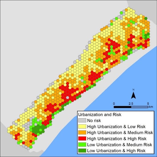
Coastal resiliency necessitates an understanding of where urban development is occurring in relationship with the level of risk. Therefore, we compared risk with urbanization to identify where current development is at risk and where potential future development may be at risk and can be protected or land use development regulations can be adopted to protect homeowners and their property. The area of urban land in 2016 was summarized to the tessellation polygons, and although there is still undeveloped land, most of the coastal area (666 tessellations or 83%) has been at least 25% developed (Figure 14). These developing hexagons are a mixture of low risk (273 or 34%), medium risk (269 or 33%), and high risk (124 or 15%), which means 48% of the study area is urban and at risk. Conversely, of the hexagons that are not yet developed (urban ≤ 25%) (138 out of 804), there are 55 (7%) that have a medium risk and 35 (4%) that have a high risk, which means that 65% of the undeveloped area is at risk and may get developed, and these places need to have careful considerations to reduce the risk to these properties.

4. Discussion

The goal was to utilize a variety of readily available data and a combination of geospatial analysis techniques to investigate the relationship between land cover change, urbanization, wetland loss, and potential flooding with respect to how these factors spatially interact. Most studies of this type have focused on a relatively small study area, such as one urban area or a bay/estuary, where the investigation identifies where changes have occurred and computes various metrics (e.g., rate of wetland loss) [30,31,32,33,34,35,36,37,38,39,40]. Conversely, in this project, we investigated a large study area (2281 km2) where we conducted a generalized/regional assessment of the changing environment and investigated a large coastal area (105 km2) in much greater detail using high-resolution data to look for patterns and trends for a variety of factors. Unlike previous studies, it is the combination of techniques that enabled the careful investigation of several changes throughout the area. We statistically tested the changes in the county versus the coast and identified that (1) the larger county area was dominated by a loss in forested area while the coast had the largest increase in urban development and (2) the change in wetlands was significantly greater along the coast in comparison with the inland part of the county.
Unlike previous research, this project utilized a vast amount of data at a very high resolution. For example, we analyzed aerial photography for the entire coastal zone including classifying the shoreline (144 km) into the type of changes that have taken place. We demonstrated that computing resources, software, data, and algorithms are fully capable of analyzing a large volume of data at multiple spatial scales to derive an understanding of the complex changes and the interplay among the various coastal processes at work in this area. Future research could build upon this multi-scale approach by using imagery obtained from unmanned aerial systems (UASs) at a very local scale where land cover and shoreline changes have been identified [41,42,43,44,45]. Instrumentation aboard unmanned aerial vehicles (UAVs) can provide excellent spatial resolution as well as multispectral bands; however, the coverage is limited because of battery time for overflights and access to launch and retrieve equipment can be problematic [44,45]. Therefore, a multi-scale approach that identifies critically changing locations is a prudent approach to identifying and ranking UAS missions.
The primary drivers of change to wetlands in a coastal environment are subsidence (which is minimal to non-existent in this study area), sea-level rise (SLR), and sedimentation. This project has documented that land cover change and urbanization along the coast has been substantial and is directly related to the natural and anthropogenic processes. Although the overall rate of change in wetlands was small (2.28% loss in wetlands along the coast), which is normal for a large study area, the location of change was significantly related to the processes that impact the coast. For example, most of the study area shoreline (100 km or 69%) had wetland loss and adjacent urban growth while a small amount (19 km or 13%) of shoreline had wetland gain in areas of urbanization which indicates that the sedimentation rate from development is keeping up with SLR. Evidence of wetland migration (22 km or 15%) demonstrated that SLR has necessitated that the environment keeps up with this rising water level, and subsequently, new wetlands/salt marsh have been established in the landward direction of the original marsh. These results confirm the conceptual model of wetland transition and migration [10,11] and the methods to derive this information. In this study area, urban expansion was the dominant detrimental impact to the coastal salt marsh; however, the variety of marsh changes provided examples of all types of coastal wetland change which demonstrates that the coastal environment is complex but directly correlated urbanization with wetland change.
The use of high spatial resolution Lidar data to derive a DEM, which was then used to identify potential places of storm-water collection/flooding, worked well in this study area. We utilized Planet satellite imagery to map water before and after a hurricane (Florence) to derive a map of floodwater, and when this was compared with DEM-derived potential stormwater collection points, these data matched well (significantly correlated) with the recent storm event. What this means is that there is value in having a historical record of flooding, but the additional topographic assessment based on a high spatial resolution DEM provides an independent predictive assessment of flood potential, which helps with planning and decision making to ameliorate stakeholders’ concerns that may negate historical events. Therefore, although each site area is different and Lidar data vary considerably, it is a useful method to potentially identify stormwater management issues. Additionally, potential stormwater depressions provide an important addition to support local government planning and the management of rapidly urbanizing areas where stormwater management is an increasing problem in many areas [46,47,48,49,50,51]. Traditionally, FEMA floodplain boundaries are the de-facto standard to measure flood risk, but they have been highly criticized and do not provide a complete picture of flood potential [52,53].
The identification of coastal risk from flooding and wetland loss documented areas that can be further investigated. For example, future analysis could incorporate the Lidar elevation data (DSM and DEM) along with the wetland maps (which were mapped using NAIP aerial photography and Lidar) and change results to further identify areas at risk to wetland loss [54]. The most popular model to assess potential changes to coastal marshes due to SLR is SLAMM (sea-level affecting marshes model) [55]; however, there is an increasing amount of evidence that the output from this model is directly related to the accuracy (horizontal and vertical) of elevation and habitat mapping data [56]. Therefore, another potential future analysis with data derived from this project will be to test the accuracy of the SLAMM model in this study area. Now that we have documented areas at risk, it will be interesting and potentially useful to see if SLAMM also identifies these same areas at risk. Considering the reliance on elevation data (which can be inaccurate [57,58,59,60,61,62,63,64,65,66,67,68,69,70,71,72,73,74,75,76,77]), many researches have questioned the validity of the SLAMM output [54,56]. For example, one major drawback of SLAMM is that it does not incorporate urban development, or other land use conversions, into the model and since this is a driver of change in this study area, another modeling option is the use of ST-SIM (state-and-transition simulation model) [78]. The advantage of ST-SIM is that the model incorporates all types of changes, or transitions, and can simulate various scenarios such as SLR, urban development, loss of forest, agriculture, wetlands, etc. The simulations can then be compared to previous historical data to validate the transitions and plan for future land use development. We are currently testing ST-SIM at various locations along the North Carolina coast, such as barrier islands and large tidal creeks, where there have been changes in the tidal freshwater habitats that have been transitioning to saltwater marshes [12,79].
With regards to urban development, this study utilized an often unused and yet valuable data source: building permits. All property owners in the United States must purchase a building permit to develop land and therefore these records can be useful, if geocoded, to identifying spatial and temporal patterns. The study area described here has been rapidly urbanizing, like most coastal areas around the world; hence, most of the area is already developed or is in the process of been converted from natural to developed land. Only 11% of the study area is less than 25% developed and yet much of this area is at risk to possible flooding, wetlands loss, and short distance to floodplains. In this study, we used a tessellation approach to quantifying coastal risk and comparing it with urban development, but there are other approaches that can be utilized. For example, a multi-criteria stochastic modeling approach is simple and popular [80,81,82,83,84,85] but runs the risk of not accounting for inherent error in spatial data. Alternatively, fuzzy set methods and change vector analysis have demonstrated utility in the coastal zone [35,36,86,87,88,89,90].

5. Conclusions

Analyzing coastal change is dependent on several factors: (1) natural and anthropogenic processes, (2) scale (spatial and temporal) of available data, and (3) techniques to identify and assess patterns and trends. In this study, we have conducted a multi-scale approach to identify coastal changes in a rapidly urbanizing area of southeastern North Carolina, USA. Urbanization is the largest driver of change where forest, agriculture, and wetlands have been replaced with urban development. Along the coast, 75% of the area and 69% of the shoreline has been urbanized while wetlands have been lost. Geocoded building permits and the calculation of change through time has identified areas of growth that provided new information not captured in the image processing and land cover change analysis.
Areas at risk were identified using Lidar data to derive depressions that are potential stormwater flooding, wetland loss which reduces the ability to ameliorate storm impacts, and distance to floodplains. These at-risk areas were compared with urbanization to reveal current problem areas and areas that are yet to be developed. These results are being used by planning officials to compare with existing planning regulations to propose new regulations to the Planning Board that will establish greater coastal resiliency through measures such as preserving wetlands, creating connected green spaces, and possibly adjusting building codes such as modifications to existing freeboard regulations which is more expensive to construct, but provides homeowners with a safer house if a flood event is to occur [91]. Additionally, Pender County is pursuing admission to FEMAs Community Rating System (CRS), which will enable county residents to participate in the National Flood Insurance Program (NFIP) at reduced rates [92,93]. However, to be granted into this program the county must meet planning standards that demonstrate that they are reducing risk to people and property. Information derived from this project is being used to apply to the CRS.
Lastly, this paper has demonstrated that the combination of image processing and geospatial analysis has identified patterns that would not be evident if only one approach had been undertaken. Investigating patterns using a variety of techniques will identify consistent patterns and specific locations where changes have occurred. Therefore, our recommendation is to utilize the data and methods described here to identify coastal changes and risk in other locations. Through this systematic approach to both raster and vector analysis, new information about coastal environments can be derived and compared. By utilizing multiple spatial analysis approaches, there can be verifiable measures of certainty and patterns in the landscape can be confirmed or reveal new information about how a place has been changing.

Author Contributions

The following contributions were made to this publication: J.N.H. conceptualized the project and designed the methodology; J.L.M. used the remote sensing and GIS software and conducted the accuracy assessment while J.N.H. conducted the formal data analysis; J.N.H. and J.L.M. collaborated on the project investigation; data curation and writing the manuscript was J.N.H. while J.N.H. and J.L.M. both created visualizations; supervision, project administration, and funding acquisition was J.N.H.

Funding

This research was funded by North Carolina Sea Grant, grant number 18-CCRG-02.

Acknowledgments

The authors would like to thank Wes Macleod and Pat O’Mahony who provided insight regarding the planning process for Pender County, North Carolina.

Conflicts of Interest

The authors declare no conflict of interest and the funders had no role in the design of the study; in the collection, analyses, or interpretation of data; in the writing of the manuscript, or in the decision to publish the results.

References

  1. McGranahan, G.; Balk, D.; Anderson, B. The rising tide: Assessing the risks of climate change and human settlements in low elevation coastal zones. Environ. Urban. 2007, 19, 17–37. [Google Scholar] [CrossRef]
  2. NOAA. National Coastal Population Report: Population Trends from 1970 to 2020; NOAA: Silver Spring, MD, USA, 2013.
  3. Deason, G.; Seekamp, E.; Barbieri, C. Perceived impacts of climate change, coastal development and policy on oyster harvesting in the Southeastern United States. Mar. Policy 2014, 50 Pt A, 142–150. [Google Scholar] [CrossRef]
  4. Carolina Demography. Are NC Growth Patterns Shifting? 2018. Available online: https://demography.cpc.unc.edu/2018/03/22/are-nc-county-growth-patterns-shifting/ (accessed on 13 February 2019).
  5. Crowell, M.; Coulton, K.; Johnson, C.; Westcott, J.; Bellomo, D.; Edehnan, S.; Hirsch, E. An Estimate of the U.S. Population Living in 100-Year Coastal Flood Hazard Areas. J. Coast. Res. 2010, 26, 201–211. [Google Scholar] [CrossRef]
  6. Zervas, C. Sea Level Variations of the United States 1854–2006; Technical Report NOS CO-OPS 053; NOAA: Silver Spring, MD, USA, 2009. Available online: https://tidesandcurrents.noaa.gov/publications/Tech_rpt_53.pdf (accessed on 26 May 2019).
  7. Church, J.A.; Clark, P.U.; Cazenave, A.; Gregory, J.M.; Jevrejeva, S.; Levermann, A.; Merrifield, M.A.; Milne, G.A.; Nerem, R.S.; Nunn, P.D.; et al. Sea Level Change. In Climate Change 2013: The Physical Science Basis. Contribution of Working Group 1 to the Fifth Assessment Report of the Intergovernmental Panel on Climate Change; Cambridge University Press: New York, NY, USA, 2013; pp. 1137–1216. Available online: https://www.researchgate.net/profile/Abha_Chhabra2/publication/271702872_Carbon_and_Other_Biogeochemical_Cycles/links/54cf9ce80cf24601c094a45e/Carbon-and-Other-Biogeochemical-Cycles.pdf (accessed on 26 May 2019).
  8. Sweet, W.V.; Kopp, R.E.; Weaver, C.P.; Obeysekera, J.; Horton, R.M.; Thieler, E.R.; Zervas, C. Global and Regional Sea Level Rise Scenarios for the United States; NOAA: Silver Spring, MD, USA, 2017.
  9. Martinez, M.; Costanza, R.; Pérez-Maqueo, O. 12.07—Ecosystem Services Provided by Estuarine and Coastal Ecosystems: Storm Protection as a Service from Estuarine and Coastal Ecosystems. In Treatise on Estuarine and Coastal Science: Volume 12—Ecological Economics of Estuaries and Coasts, 1st ed.; van den Belt, M., Costanza, R., Eds.; Academic Press: Cambridge, MA, USA, 2011; pp. 129–146. [Google Scholar]
  10. Weigert, R.G.; Freeman, B.J. Tidal Salt Marshes of the Southeast Atlantic Coast: A Community Profile; Wetland and Aquatic Research Center: Gainesville, FL, USA, 1990; p. 80.
  11. Stammermann, R.; Piasecki, M. Influence of sediment availability, vegetation, and sea level rise on the development of tidal marshes. J. Coast. Res. 2012, 28, 1536–1549. [Google Scholar] [CrossRef]
  12. Ensign, S.H.; Noe, G.B. Tidal extension and sea-level rise: Recommendations for a research agenda. Front. Ecol. Environ. 2018, 16, 37–43. [Google Scholar] [CrossRef]
  13. Ferrer-Valero, N.; Hernandez-Calvento, L.; Hernandez-Cordero, A.I. Human impacts quantification on the coastal landforms of Gran Canaria Island (Canary Islands). Geomorphology 2017, 286, 58–67. [Google Scholar] [CrossRef]
  14. McCarthy, M.J.; Colna, K.E.; El-Mezayen, M.M.; Laureano-Rosario, A.E.; Mendez-Lazaro, P.; Otis, D.B.; Toro-Farmer, G.; Vega-Rodriguez, M.; Muller-Karger, F.E. Satellite Remote Sensing for Coastal Management: A Review of Successful Applications. Environ. Manag. 2017, 60, 323–339. [Google Scholar] [CrossRef] [PubMed]
  15. USGS. National Hydrography Dataset; US Department of the Interior, Ed.; USGS: Reston, VA, USA, 2018.
  16. FEMA. FEMA Flood Map Service Center; Department of Homeland Security: Washington, DC, USA. Available online: https://msc.fema.gov/portal/home (accessed on 9 November 2017).
  17. NOAA. C-CAP Southeast Region 1996-2010-Era Land Cover Change. Available online: www.coast.noaa.gov/ccapftp (accessed on 1 May 2018).
  18. O’Mahony, P. Pender County GIS Data: Residential Building Permits, Zoning, and Parcels; County, P., Ed.; Burgaw, NC, USA, 2018. [Google Scholar]
  19. NC Department of Emergency Management. QL2 LiDAR. Available online: https://sdd.nc.gov/sdd/ (accessed on 16 February 2019).
  20. Planet. Planet Application Program Interface: In Space for Life on Earth. Available online: https://www.planet.com/ (accessed on 1 October 2018).
  21. USGS. Digital Orthophoto Quadrangle (DOQs). Available online: https://earthexplorer.usgs.gov/ (accessed on 1 October 2019).
  22. Esri. Creating Raster DEMs and DSMs from Large Lidar Point Collections. Available online: http://desktop.arcgis.com/en/arcmap/10.5/manage-data/las-dataset/lidar-solutions-creating-raster-dems-and-dsms-from-large-lidar-point-collections.htm (accessed on 28 May 2019).
  23. American Society of Photogrammetry & Remote Sensing (ASPRS). LAS Specification 1.4—R14. Available online: http://www.asprs.org/wp-content/uploads/2019/03/LAS_1_4_r14.pdf (accessed on 12 July 2019).
  24. National Weather Service. Historical Hurricane Florence, 12–15 September 2018. Available online: https://www.weather.gov/mhx/Florence2018 (accessed on 29 October 2018).
  25. National Weather Service. Wilmington’s Race to 100 Inches! Available online: https://www.weather.gov/ilm/Raceto100 (accessed on 21 June 2019).
  26. Gao, B. NDWI—A normalized difference water index for remote sensing of vegetation liquid water from space. Remote Sens. Environ. 1996, 58, 257–266. [Google Scholar] [CrossRef]
  27. USDA. National Agriculture Imagery Program (NAIP). Available online: https://www.fsa.usda.gov/programs-and-services/aerial-photography/imagery-programs/naip-imagery/ (accessed on 1 October 2018).
  28. Trimble Geospatial. eCognition Essentials, Version 1.3. 2019. Available online: http://www.ecognition.com/ (accessed on 21 June 2018).
  29. Dupuy, S.; Barbe, E.; Balestrat, M. An Object-Based Image Analysis Method for Monitoring Land Conversion by Artificial Sprawl Use of RapidEye and IRS Data. Remote Sens. 2012, 4, 404–423. [Google Scholar] [CrossRef] [Green Version]
  30. Campbell, A.; Wang, Y. High Spatial Resolution Remote Sensing for Salt Marsh Mapping and Change Analysis at Fire Island National Seashore. Remote Sens. 2019, 11, 1107. [Google Scholar] [CrossRef]
  31. Campbell, A.; Wang, Y.; Christiano, M.; Stevens, S. Salt Marsh Monitoring in Jamaica Bay, New York from 2003 to 2013: A Decade of Change from Restoration to Hurricane Sandy. Remote Sens. 2017, 9, 131. [Google Scholar] [CrossRef]
  32. Gorman, L.; Morang, A.; Larson, R. Monitoring the Coastal Environment; Part IV: Mapping, Shoreline Change, and Bathymetric Analysis. J. Coast. Res. 1998, 14, 61–92. [Google Scholar]
  33. Chen, Y.B.; Wu, Z.F.; Qian, Q.L.; Zheng, Z.H.; Han, F.H. Dynamic monitoring and spatiotemporal evolution of the coastline in Pearl River Estuary in recent fifty years. In 2016 4th International Workshop on Earth Observation and Remote Sensing Applications; Weng, Q., Gamba, P., Xian, G., Chen, J.M., Liang, S., Eds.; CRC Press: Guangzhou, China, 2016; China ISBN 978-1-5090-1479-8. [Google Scholar]
  34. Crawford, T.W.; Marcucci, D.J.; Bennett, A. Impacts of residential development on vegetation cover for a remote coastal barrier in the Outer Banks of North Carolina, USA. J. Coast. Conserv. 2013, 17, 431–443. [Google Scholar] [CrossRef]
  35. Dewi, R.S.; Bijker, W.; Stein, A.; Marfai, M.A. Fuzzy Classification for Shoreline Change Monitoring in a Part of the Northern Coastal Area of Java, Indonesia. Remote Sens. 2016, 8, 190. [Google Scholar] [CrossRef]
  36. Dewi, R.S.; Bijker, W.; Stein, A. Change Vector Analysis to Monitor the Changes in Fuzzy Shorelines. Remote Sens. 2017, 9, 147. [Google Scholar] [CrossRef]
  37. Domingues, R.B.; Santos, M.C.; de Jesus, S.N.; Ferreira, O. How a coastal community looks at coastal hazards and risks in a vulnerable barrier island system (Faro Beach, southern Portugal). Ocean Coast. Manag. 2018, 157, 248–256. [Google Scholar] [CrossRef]
  38. De Sanjosé Blasco, J.J.; Gómez-Lende, M.; Sánchez-Fernández, M.; Serrano-Cañadas, E. Monitoring Retreat of Coastal Sandy Systems Using Geomatics Techniques: Somo Beach (Cantabrian Coast, Spain, 1875–2017). Remote Sens. 2018, 10, 1500. [Google Scholar] [CrossRef]
  39. Grybas, H.; Congalton, G.R. Land Cover Change Image Analysis for Assateague Island National Seashore Following Hurricane Sandy. J. Imaging 2015, 1, 85–114. [Google Scholar] [CrossRef] [Green Version]
  40. McCarthy, M.; Halls, J. Habitat Mapping and Change Assessment of Coastal Environments: An Examination of WorldView-2, QuickBird, and IKONOS Satellite Imagery and Airborne LiDAR for Mapping Barrier Island Habitats. ISPRS Int. J. Geo-Inf. 2014, 3, 297–325. [Google Scholar] [CrossRef] [Green Version]
  41. Duo, E.; Trembanis, A.; Dohner, S.; Grottoli, E.; Ciavola, P. Local-scale post-event assessments with GPS and UAV-based quick-response surveys: A pilot case from the Emilia-Romagna (Italy) coast. Nat. Hazards Earth Syst. Sci. 2018, 18, 2969–2989. [Google Scholar] [CrossRef]
  42. Long, N.; Millescamps, B.; Guillot, B.; Pouget, F.; Bertin, X. Monitoring the Topography of a Dynamic Tidal Inlet Using UAV Imagery. Remote Sens. 2016, 8, 387. [Google Scholar] [CrossRef]
  43. Long, N.; Millescamps, B.; Pouget, F.; Dumon, A.; Lachaussee, N.; Bertin, X. Accuracy Assessment of Coastal Topography Derived from UAV Images. In Proceedings of the International Archives of the Photogrammetry, Remote Sensing and Spatial Information Sciences, Volume XLI-B1, 2016 XXIII ISPRS Congress, Prague, Czech Republic, 12–19 July 2016; 41, pp. 1127–1134. [Google Scholar] [CrossRef]
  44. Goncalves, J.A.; Henriques, R. UAV photogrammetry for topographic monitoring of coastal areas. ISPRS J. Photogramm. Remote Sens. 2015, 104, 101–111. [Google Scholar] [CrossRef]
  45. Klemas, V.V. Coastal and Environmental Remote Sensing from Unmanned Aerial Vehicles: An Overview. J. Coast. Res. 2015, 31, 1260–1267. [Google Scholar] [CrossRef]
  46. Sarmah, T.; Das, S. Urban flood mitigation planning for Guwahati: A case of Bharalu basin. J. Environ. Manag. 2018, 206, 1155–1165. [Google Scholar] [CrossRef]
  47. Brody, S.D.; Highfield, W.E.; Blessing, R.; Makino, T.; Shepard, C.C. Evaluating the effects of open space configurations in reducing flood damage along the Gulf of Mexico coast. Landsc. Urban Plan. 2017, 167, 225–231. [Google Scholar] [CrossRef]
  48. Passeri, D.L.; Hagen, S.C.; Medeiros, S.C.; Bilskie, M.V.; Alizad, K.; Wang, D.B. The dynamic effects of sea level rise on low-gradient coastal landscapes: A review. Earths Future 2015, 3, 159–181. [Google Scholar] [CrossRef]
  49. Brody, S.D.; Blessing, R.; Sebastian, A.; Bedient, P. Delineating the Reality of Flood Risk and Loss in Southeast Texas. Nat. Hazards Rev. 2013, 14, 89–97. [Google Scholar] [CrossRef]
  50. Czajkowski, J.; Kunreuther, H.; Michel-Kerjan, E. Quantifying Riverine and Storm-Surge Flood Risk by Single-Family Residence: Application to Texas. Risk Anal. 2013, 33, 2092–2110. [Google Scholar] [CrossRef] [Green Version]
  51. Santos, M.; del Río, L.; Benavente, J. GIS-based approach to the assessment of coastal vulnerability to storms. Case study in the Bay of Cádiz (Andalusia, Spain). J. Coast. Res. 2013, 1, 826–831. [Google Scholar] [CrossRef]
  52. Shively, D. Flood risk management in the USA: Implications of national flood insurance program changes for social justice. Reg. Environ. Chang. 2017, 17, 2323. [Google Scholar] [CrossRef]
  53. Crowell, M.; Hirsch, E.; Hayes, T.L. Improving FEMA’s coastal risk assessment through the National Flood Insurance Program: An historical overview. Mar. Technol. Soc. J. 2007, 41, 18–27. [Google Scholar] [CrossRef]
  54. Ekberg, M.L.C.; Raposa, K.B.; Ferguson, W.S.; Ruddock, K.; Watson, E.B. Development and Application of a Method to Identify Salt Marsh Vulnerability to Sea Level Rise. Estuaries Coasts 2017, 40, 694–710. [Google Scholar] [CrossRef]
  55. Warren Pinnacle Consulting. SLAMM: Sea Level Affecting Marshes Model. Available online: http://warrenpinnacle.com/prof/SLAMM/index.html (accessed on 19 June 2019).
  56. Fernandez-Nunez, M.; Burningham, H.; Díaz-Cuevas, P.; Ojeda-Zújar, J. Evaluating the Response of Mediterranean-Atlantic Saltmarshes to Sea-Level Rise. Resources 2019, 8, 50. [Google Scholar] [CrossRef]
  57. Cooper, H.M.; Zhang, C.Y.; Davis, S.E.; Troxler, T.G. Object-based correction of LiDAR DEMs using RTK-GPS data and machine learning modeling in the coastal Everglades. Environ. Model. Softw. 2019, 112, 179–191. [Google Scholar] [CrossRef]
  58. Enwright, N.M.; Wang, L.; Borchert, S.M.; Day, R.H.; Feher, L.C.; Osland, M.J. Advancing barrier island habitat mapping using landscape position information. Prog. Phys. Geogr. Earth Environ. 2019, 43, 425–450. [Google Scholar] [CrossRef]
  59. Schmelz, W.J.; Psuty, N.P. Quantification of Airborne Lidar Accuracy in Coastal Dunes (Fire Island, New York). Photogramm. Eng. Remote Sens. 2019, 85, 133–144. [Google Scholar] [CrossRef]
  60. Watson, E.B.; Haaf, L.; Raper, K.; Reilly, E. Removal of Positive Elevation Bias of Digital Elevation Models for Sea-Level Rise Planning. Data 2019, 4, 46. [Google Scholar] [CrossRef]
  61. Enwright, M.N.; Wang, L.; Borchert, M.S.; Day, H.R.; Feher, C.L.; Osland, J.M. The Impact of Lidar Elevation Uncertainty on Mapping Intertidal Habitats on Barrier Islands. Remote Sens. 2018, 10, 5. [Google Scholar] [CrossRef]
  62. Gesch, D.B. Best Practices for Elevation-Based Assessments of Sea-Level Rise and Coastal Flooding Exposure. Front. Earth Sci. 2018, 6, 19. [Google Scholar] [CrossRef]
  63. Halls, J.N.; Frishman, M.A.; Hawkes, A.D. An Automated Model to Classify Barrier Island Geomorphology Using Lidar Data and Change Analysis (1998–2014). Remote Sens. 2018, 10, 1109. [Google Scholar] [CrossRef]
  64. Nie, S.; Wang, C.; Xi, X.; Luo, S.; Li, S.; Tian, J. Estimating the height of wetland vegetation using airborne discrete-return LiDAR data. Optik 2018, 154, 267–274. [Google Scholar] [CrossRef]
  65. O’Neil, G.; Goodall, J.; Watson, L. Evaluating the potential for site-specific modification of LiDAR DEM derivatives to improve environmental planning-scale wetland identification using Random Forest classification. J. Hydrol. 2018, 559, 192–208. [Google Scholar] [CrossRef]
  66. Popescu, G.; Iordan, D. An Overall View of Lidar and Sonar Systems Used in Geomatics Applications for Hydrology. Sci. Pap. Ser. E-Land Reclam. Earth Obs. Surv. Environ. Eng. 2018, 7, 174–181. [Google Scholar]
  67. Rapinel, S.; Clement, B.; Dufour, S.; Hubert-Moy, L. Fine-Scale Monitoring of Long-term Wetland Loss Using LiDAR Data and Historical Aerial Photographs: The Example of the Couesnon Floodplain, France. Wetlands 2018, 38, 423–435. [Google Scholar] [CrossRef]
  68. Xu, H.; Hodgson, M.; Piovan, S.; Tufford, D. The potential of using LiDAR and color-infrared aerial imagery for palustrine wetland typology and change. GIsci. Remote Sens. 2018, 55, 477–501. [Google Scholar] [CrossRef]
  69. Ye, S.; Pontius, R.G.; Rakshit, R. A review of accuracy assessment for object-based image analysis: From per-pixel to per-polygon approaches. ISPRS J. Photogramm. Remote Sens. 2018, 141, 137–147. [Google Scholar] [CrossRef]
  70. Rogers, J.N.; Parrish, C.E.; Ward, L.G.; Burdick, D.M. Assessment of Elevation Uncertainty in Salt Marsh Environments using Discrete-Return and Full-Waveform Lidar. J. Coast. Res. 2016, 76, 107–122. [Google Scholar] [CrossRef] [Green Version]
  71. Medeiros, S.; Hagen, S.; Weishampel, J.; Angelo, J. Adjusting Lidar-Derived Digital Terrain Models in Coastal Marshes Based on Estimated Aboveground Biomass Density. Remote Sens. 2015, 7, 3507–3525. [Google Scholar] [CrossRef] [Green Version]
  72. Rogers, J.; Parrish, C.E.; Ward, L.G.; Burdick, D.M. Evaluation of field-measured vertical obscuration and full waveform lidar to assess salt marsh vegetation biophysical parameters. Remote Sens. Environ. 2015, 156, 264–275. [Google Scholar] [CrossRef]
  73. Coveney, S. Association of elevation error with surface type, vegetation class and data origin in discrete-returns airborne LiDAR. Int. J. Geogr. Inf. Sci. 2013, 27, 467–483. [Google Scholar] [CrossRef]
  74. Pe’eri, S.; Long, B. LIDAR Technology Applied in Coastal Studies and Management. J. Coast. Res. 2011, 62, 1–5. [Google Scholar] [CrossRef]
  75. Schmid, K.A.; Hadley, B.C.; Wijekoon, N. Vertical Accuracy and Use of Topographic LIDAR Data in Coastal Marshes. J. Coast. Res. 2011, 27, 116–132. [Google Scholar] [CrossRef]
  76. Rayburg, S.; Thoms, M.; Neave, M. A comparison of digital elevation models generated from different data sources. Geomorphology 2009, 106, 261–270. [Google Scholar] [CrossRef]
  77. Hogg, A.; Holland, J. An evaluation of DEMs derived from LiDAR and photogrammetry for wetland mapping. For. Chron. 2008, 84, 840–849. [Google Scholar] [CrossRef] [Green Version]
  78. Daniel, C.J.; Frid, L.; Sleeter, B.M.; Fortin, M.J. State-and-transition simulation models: A framework for forecasting landscape change. Methods Ecol. Evol. 2016, 7, 1413–1423. [Google Scholar] [CrossRef]
  79. Alizad, K.; Hagen, S.C.; Morris, J.T.; Medeiros, S.C.; Bilskie, M.V.; Weishampel, J.F. Coastal wetland response to sea-level rise in a fluvial estuarine system. Earths Future 2016, 4, 483–497. [Google Scholar] [CrossRef]
  80. Kombiadou, K.; Matias, A.; Carrasco, R.; Ferreira, O.; Costas, S.; Vieira, G. Towards Assessing the Resilience of Complex Coastal Systems: Examples from Ria Formosa (South Portugal). J. Coast. Res. 2018, 646–650. [Google Scholar] [CrossRef]
  81. Rincón, D.; Khan, U.; Armenakis, C. Flood Risk Mapping Using GIS and Multi-Criteria Analysis: A Greater Toronto Area Case Study. Geosciences 2018, 8, 275. [Google Scholar] [CrossRef]
  82. Dunkin, L.; Reif, M.; Altman, S.; Swannack, T. A Spatially Explicit Multi-Criteria Decision Support Model for Loggerhead Sea Turtle Nesting Habitat Suitability: A Remote Sensing-Based Approach. Remote Sens. 2016, 8, 573. [Google Scholar] [CrossRef]
  83. Cabrera-Barona, P.; Murphy, T.; Kienberger, S.; Blaschke, T. A multi-criteria spatial deprivation index to support health inequality analyses. Int. J. Health Geogr. 2015, 14. [Google Scholar] [CrossRef]
  84. Félix, A.; Baquerizo, A.; Santiago, J.M.; Losada, M.A. Coastal zone management with stochastic multi-criteria analysis. J. Environ. Manag. 2012, 112, 252–266. [Google Scholar] [CrossRef]
  85. Hongoh, V.; Hoen, A.G.; Aenishaenslin, C.; Waaub, J.P.; Belanger, D.; Michel, P.; Lyme, M.C. Spatially explicit multi-criteria decision analysis for managing vector-borne diseases. Int. J. Health Geogr. 2011, 10. [Google Scholar] [CrossRef]
  86. Sarkar, S.; Parihar, S.M.; Dutta, A. Fuzzy risk assessment modelling of East Kolkata Wetland Area: A remote sensing and GIS based approach. Environ. Model. Softw. 2016, 75, 105–118. [Google Scholar] [CrossRef]
  87. Jadidi, A.; Mostafavi, M.A.; Bedard, Y.; Shahriari, K. Spatial Representation of Coastal Risk: A Fuzzy Approach to Deal with Uncertainty. ISPRS Int. J. Geo-Inf. 2014, 3, 1077–1100. [Google Scholar] [CrossRef]
  88. Grekousis, G.; Thomas, H. Comparison of two fuzzy algorithms in geodemographic segmentation analysis: The Fuzzy C-Means and Gustafson–Kessel methods. Appl. Geogr. 2012, 34, 125–136. [Google Scholar] [CrossRef]
  89. Coppi, R.; D’Urso, P.; Giordani, P. A Fuzzy Clustering Model for Multivariate Spatial Time Series. J. Classif. 2010, 27, 54–88. [Google Scholar] [CrossRef]
  90. Sriti, M.; Thibaud, R.; Claramunt, C. A fuzzy identity-based temporal GIS for the analysis of geomorphometry changes. In Journal on Data Semantics III; Spaccapietra, S., Zimanyi, E., Eds.; Lecture Notes in Computer Science; Springer: Berlin/Heidelberg, Germany, 2005; Volume 3534, pp. 81–99. [Google Scholar]
  91. Xian, S.Y.; Lin, N.; Kunreuther, H. Optimal house elevation for reducing flood-related losses. J. Hydrol. 2017, 548, 63–74. [Google Scholar] [CrossRef] [Green Version]
  92. Silvis, V.G. Flooding by Design: A Look at the National Flood Insurance Program. Risk Hazards Crisis Public Policy 2018, 9, 82–99. [Google Scholar] [CrossRef]
  93. Stroud, D.A.; ASFPM. The NFIP’s Community Rating System: A Proactive Approach to Mitigation Planning; Association State Floodplain Managers, Inc.: Madison, WI, USA, 1999; pp. 41–44. [Google Scholar]
Figure 1. The study area is Pender County in Southeastern North Carolina (NC), in the Southeastern United States. The study area included two scales: (1) county-wide analysis and (2) higher spatial resolution along the coast (outlined in yellow) east of Highway 17 and west of the Intracoastal Waterway. (Data sources: NC Department of Transportation, Pender County zoning, and US Geological Survey).
Remotesensing 11 02260 g001
Figure 2. North Carolina population change (2016 to 2017). (Data source: US Census).
Remotesensing 11 02260 g002
Figure 3. Project flowchart illustrating the methods for analyzing Hurricane Florence floodwater and potential storm-water depressions (blue), classifying wetlands and computing change through time (green), and identifying urbanization and coastal risk (orange).
Remotesensing 11 02260 g003
Figure 4. Hurricane Florence (September 14, 2018) flood inundation. (Data sources: NC Department of Transportation (roads and municipalities) and PlanetScope imagery).
Remotesensing 11 02260 g004
Figure 5. Example imagery from the National Agriculture Imagery Program (NAIP) (left) and PlanetScope imagery from Planet (right) for a portion of coastal Pender County.
Remotesensing 11 02260 g005
Figure 6. Hurricane Florence (September 2018) caused extensive inland flooding (122 km2), but much less flooding (only 1.07 km2 or less than 1%) along the coast.
Remotesensing 11 02260 g006
Figure 7. Land cover change (1996 to 2010) illustrating forest (green) and wetland (magenta) loss and undeveloped areas that have become developed (red). (Data Source: C-CAP).
Remotesensing 11 02260 g007
Figure 8. Coastal land cover classification where (A) is the 2016 land cover dominated by widespread new urban development (red) and (B) is a closer look at new urban development from 1980 to 2016 where the main loss to urban areas was forest (green) and agriculture (yellow).
Remotesensing 11 02260 g008
Figure 9. Coastal shoreline classifications where each 1000 m segment was assigned a type of wetland change depending on the adjacent land cover change. The dominant change was wetland loss and urban growth (100 km), but there are smaller areas that had other changes. For example, (A) and (B) are examples of tidal creeks that had a variety of changes including wetland migration, and (C) illustrates a closer look at wetland migration where marsh loss was accompanied with wetland gain on the inland side.
Remotesensing 11 02260 g009
Figure 10. Locations of residential building permits from 2006 through 2017 (A) and a closer view of the permits in the urbanizing coastal area (B).
Remotesensing 11 02260 g010
Figure 11. Number of residential building permits (from 2006 through 2017) (A) and rate of new residential construction (slope of the regression line) for each hexagon (B). Increasing rates of permits through time have a positive slope (shown in orange and red).
Remotesensing 11 02260 g011
Figure 12. Amount of developed land cover in 2016 (A) and percent change from 1980 to 2016 (B). (Data source: NAIP).
Remotesensing 11 02260 g012
Figure 13. Flood risk in the coastal area is a combination of area of surface depressions (A), distance to floodplain (B), and area of wetlands (C). The total risk is a sum of the rankings for each of these factors (D).
Remotesensing 11 02260 g013
Figure 14. Urbanization (percent) compared with risk: places with at least 25% development (2016) or increasing development (slope greater than 0.1) of medium risk (orange) or high risk (red) and places with low development (less than 25 percent) of medium (light green) or high risk (dark green).
Remotesensing 11 02260 g014
Table 1. List of data sources and their purpose.
ProviderDataFormatMap Scale/Image ResolutionPurpose
US Geological SurveyNational Hydrology Dataset [15]Vector (lines & polygons)1:12,000Compared shoreline change
Federal Emergency Management AgencyNational Flood Hazard Layer [16]Vector (polygons)1:12,000Determined distance of land cover change, urban growth, and depressions to the 100-year floodplain
National Oceanic Atmospheric Administration (NOAA) Digital CoastCoastal Change Analysis Program (C-CAP) [17]Raster30 × 30 mComputed change in wetlands from 1996 to 2010
Pender County, North Carolina (NC)Residential Building Permits [18]AddressesUnknownIdentified residential development from 2006 through 2017
NC Department of Emergency ManagementQL2 Lidar [19]Raster1.5 × 1.5 mCreated a DEM to identify areas at risk to flooding and DSM and DEM were used to assist with classifying wetlands
PlanetPlanetScope imagery [20]Raster multi-spectral3 × 3 mIdentified flooded areas from Hurricane Florence
US Department of Agriculture Farm Service AgencyDigital Orthophotography [21]Raster1 × 1 mClassified wetlands from 1980 and 2016 imagery and computed change
Table 2. Residential building permits (2006–2017): geocoding results.
YearNumber of RecordsNumber of Geocoded RecordsPercent Geocoded
200665558689.47
200755348888.25
200836531285.48
200922419687.50
201023520988.94
201124621386.59
201232328187.00
201338134991.60
201443540192.18
201553851395.35
201657453493.03
201752547390.10
Table 3. Amount of potential stormwater depressions by land cover type (2010).
General Land Cover ClassLand Cover ClassArea (ha)Total Area (ha)Percent (%)
DevelopedHigh Intensity Developed0.010.6550.09
Medium Intensity Developed0.023
Low Intensity Developed0.084
Developed Open Space0.538
AgricultureCultivated0.54610.23113.67
Pasture/Hay9.665
Grassland0.02
ForestDeciduous Forest3.09617.21123.00
Evergreen Forest0.11
Mixed Forest14.005
Scrub/ShrubScrub/Shrub1.0881.0881.45
WetlandPalustrine Forested Wetland8.38544.64359.30
Palustrine Scrub/Shrub Wetland26.052
Palustrine Emergent Wetland8.085
Estuarine Scrub/Shrub Wetland2.111
Estuarine Emergent Wetland0.01
BareUnconsolidated Shore0.6670.670.89
Bare Land0.003
WaterWater0.3180.3180.42
Total74.816
Table 4. Percent Change in Land Cover for Pender County and Coastal Pender County (1996–2010) (Data source: C-CAP).
Pender CountyCoastal Pender County
Land Cover Type1996 (Percent)2010 (Percent)Change (2010–1996)1996 (Percent)2010 (Percent)Change (2010–1996)
Developed2.703.380.6819.0625.636.57
Agriculture17.0718.451.3817.3514.18−3.17
Forest28.3523.96−4.3914.5615.220.66
Scrub/Shrub11.6114.592.9812.209.65−2.55
Wetland37.6436.62−1.0231.5629.28−2.28
Bare0.460.810.350.100.900.80
Water2.152.210.065.165.15−0.01
Table 5. Land Cover Change Matrix (in percent): 1996–2010. (Data source: C-CAP).
2010
DevelopedAgricultureForestScrub/ShrubWetlandBareWaterTotal (1996)
1996Developed2.700.000.000.000.000.000.002.70
Agriculture0.3214.990.291.240.150.060.0117.07
Forest0.132.5721.603.820.040.180.0128.35
Scrub/Shrub0.120.621.828.750.170.130.0111.61
Wetland0.110.230.240.7636.180.070.0537.64
Bare0.000.020.000.000.040.360.040.46
Water0.000.000.000.000.040.012.092.15
Total (2010)3.3818.4523.9614.5936.620.812.21100.00
Table 6. Land Cover Change Matrix (in percent) for Coastal Pender County: 1980–2016. (Data source: NAIP).
2016
DevelopedAgricultureForestWetlandsWaterTotal (1980)
1980Developed9.520.112.820.140.1012.69
Agriculture6.860.663.980.020.0811.60
Forest18.812.4742.410.490.4064.58
Wetlands0.100.000.161.270.341.88
Water0.110.000.150.848.159.25
Total (2016)35.403.2449.532.769.08100.00
Table 7. Rate of change in building permits (2009 to 2017) and distance to floodplain.
Distance (m) from 100-yr Floodplain
Slope (Rate Change)0 *50010002000Over 2000
Number of hexagons–0.301000
–0.29 to –0.051514741
–0.04 to −0.052531251121168
–0.06 to 0.3058441251
0.31 to 2.081112500
Total33719613612510
Percent41.90%24.40%16.90%15.50%1.20%
* Distance of “0” indicates these building permits were located within the floodplain.

