1. Introduction
AR is considered as a technology that overlays virtual objects (augmented components) onto the real world [
1]. To date, AR, which recently has advanced greatly, demonstrates impressive performance in Artificial Intelligence (AI) applications, including areas in remote sensing [
2,
3,
4,
5], education [
1,
6,
7], medicine [
8,
9,
10], etc. Moreover, virtual–real registration is a critical technique and a fundamental problem for AR. The virtual–real registration process is defined as the superimposing of virtual objects onto a real scene using information extracted from the scene [
11,
12]. In detail, AR virtual–real registration is the degree to which 3D information is accurately placed and integrated as part of the real environment [
13]. The objects in the real and 3D scene should be correctly aligned with respect to each other, or the illusion that the two co-exist is compromised [
14]. Thus, the performance of AR strongly depends on the accuracy of virtual–real registration.
Nowadays, most AR virtual–real registration algorithms are normally applied to indoor environments; few are applied to outdoor environments. Uncontrolled factors and complexity of large scale data (such as hundreds of objects, dramatic changes in illumination, etc.) result in outdoor environments being uncontrolled scenes. Thus, it is very challenging to achieve virtual–real registration of AR in large-scale outdoor environments.
In this paper, based on the following two factors, we developed a novel solution for the virtual–real registration of AR in outdoor environments: (1) Aerial images, captured by Unmanned Aerial Vehicles (UAVs), provide sufficient data (vertical and oblique aerial images) for large-scale 3D image-based point clouds using Structure-from-Motion (SfM) [
15,
16] algorithms. Because of the development of low-cost UAVs and light weight imaging sensors in the past decade [
17], this 3D image-based point cloud becomes feasible and provides basic 3D information for outdoor environments for AR applications. (2) Real images captured from ground mobile devices, called ground camera images, provide an important clue for estimating the initial location and orientation of a user in the 3D environment. The overview of the proposed AR virtual–real registration approach in outdoor environments is shown in
Figure 1.
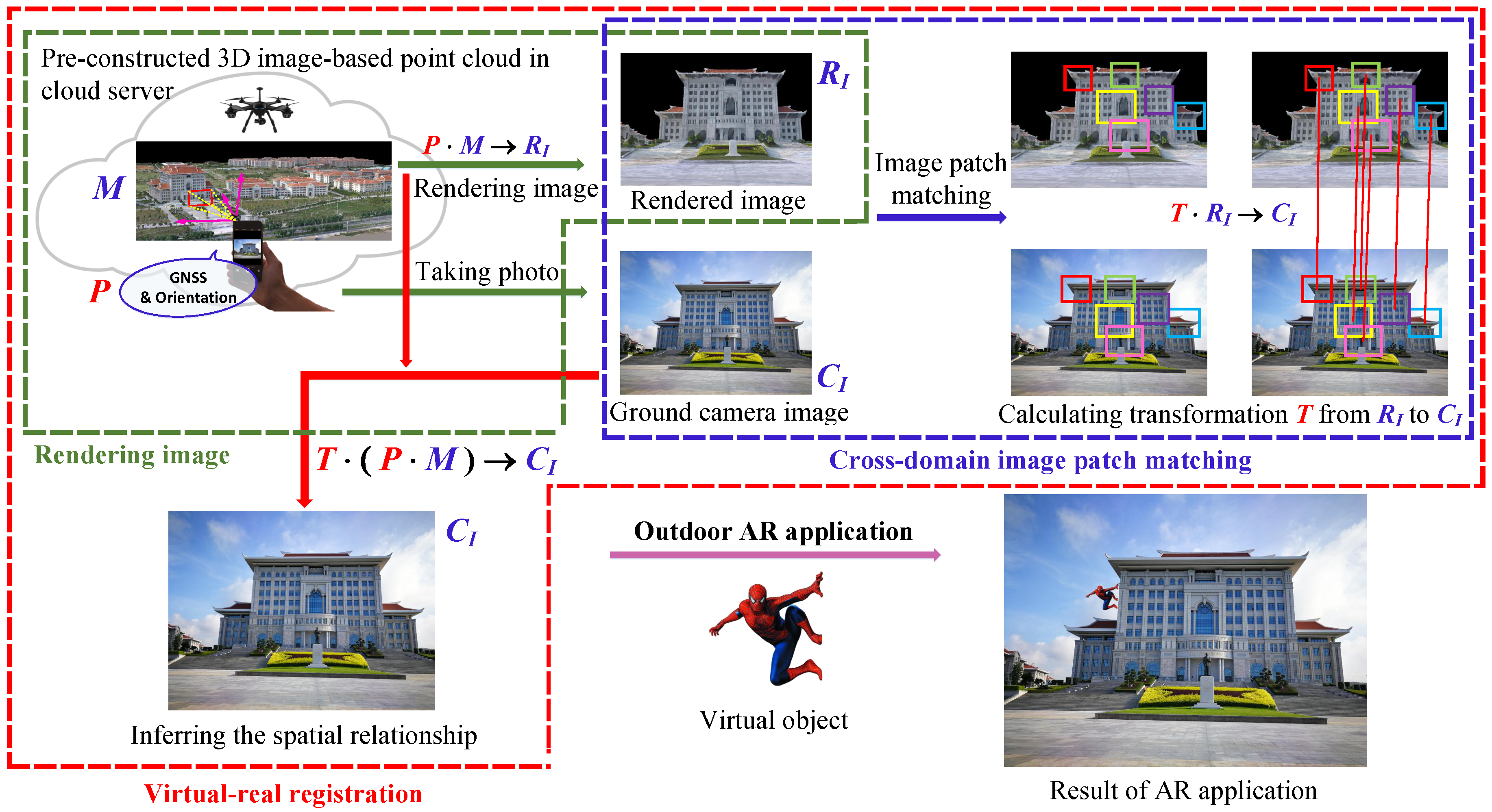
The four stages in the pipeline for the proposed virtual–real registration of AR in outdoor environments (
Figure 1) are as follows: (1) Aerial images, captured by UAVs, are used to generate a 3D image-based point cloud in urban environments via SfM technology. (2) Camera pose, acquired from a Global Navigation Satellite System (GNSS) and Inertial Measurement Units (IMU) from mobile devices as an initial estimate, is used to synthesize an image, which is rendered from the same viewpoint as the 3D image-based point cloud (In this paper, we call this synthetic image as ’rendered image’). A schematic of the rendering process is shown within the green dashed bounding box in
Figure 1. (3) A ground camera image and the rendered image are matched by using the invariant feature descriptors, which are learned by our proposed AE-GAN-Net. The details are discussed in the following Section. Then, the above matching results are used to indirectly infer the spatial relationship between the 3D image-based point cloud and ground camera image. The schematic of the image patch matching process is shown within the blue dashed bounding box in
Figure 1. (4) Using the following strategy, virtual object (Spiderman in
Figure 1) is registered to a real scene by: first, determine where the virtual object (Spiderman) is to be placed in the 3D image-based point cloud; second, by using the inferred spatial relationship between 3D and 2D space, the virtual object (Spiderman) is registered to the cellphone image.
In detail, the inference of the spatial relationship is shown within the red dashed bounding box in
Figure 1. The 3D image-based point cloud, ground camera image, and rendered image are denoted as
M,
,
, respectively; the projection matrix from the 3D image-based point cloud to the rendered image is denoted as
P (
P is positioning information obtained from the mobile devices). Intuitively, the relationship between the 3D image-based point cloud and the rendered image is
. Then, supposing the transformation relationship from the rendered image to the ground camera image is
T, the result is
. Thus, the spatial relationship between the 3D image-based point cloud and the ground camera image (3D space and 2D space) is indirectly inferred as
.
Essentially, the core problem for the proposed virtual real registration is to estimate the above assuming transformation matrix, T, from the rendered image to the ground camera image. Thus, our motivation is to indirectly establish the spatial relationship between 2D and 3D space by matching the ground camera images to the corresponding rendered images. It should be noted that the imaging mechanisms and nature of ground camera images and rendered images are different; thus, we consider them as cross-domain images.
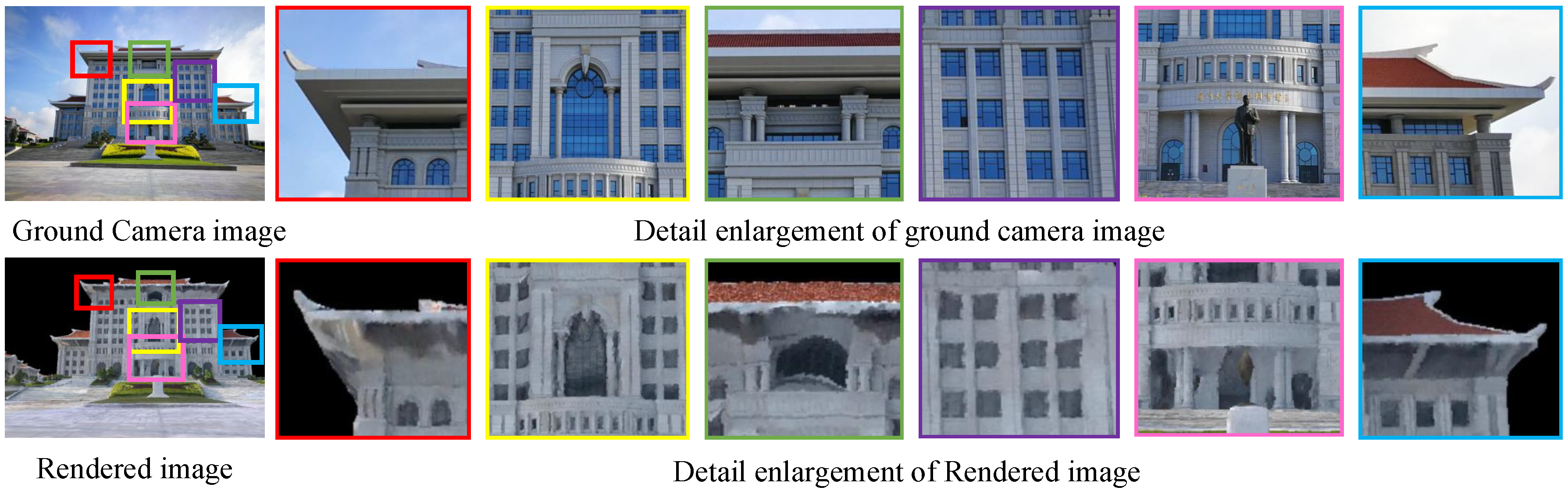
However, for the following three reasons, it is challenging to match the ground camera images and the rendered images: (1) These two kinds of cross-domain images tend to have a gap in different local appearances. This characteristic data gap of different domains is the major difficulty for measuring the similarity of the features extracted from different domain images. (2) The rendered images from the 3D image-based point cloud have bias and drift from the corresponding ground camera images, because the position information from the mobile phone is an initial and coarse estimation. (3) It is difficult for the outdoor aerial images captured by UAVs to cover all terrain details (e.g., the structures under the eaves, the bottoms of buildings, and objects close to the ground). So the quality of the 3D image-based point cloud reconstructed by the SfM algorithm is inadequate. Therefore, rendered images, which have large distortion, low resolution, structural repetitiveness, and occlusions, are generally of low quality (See
Figure 2). Thus, the image matching between ground camera images and rendered images is beyond the reach of the handcrafted features, such as Scale Invariant Feature Transform (SIFT) [
18], Speeded Up Robust Features (SURF) [
19], Efficient Dense Descriptor Applied to Wide-baseline Stereo (DAISY) [
20], Oriented FAST and Rotated BRIEF (ORB) [
21], etc. Some failed matching results are shown in
Figure 3.
As seen in
Figure 3a, the extracted keypoints of the ground camera images are robust. In contrast, a 3D image-based point cloud generated by the SfM algorithm has distortion and low resolution, which causes the surface of the 3D model to be coarse. Thus, the synthetic images rendered from the 3D image-based point cloud are low quality, and the texture of the rendered images is coarse. Consequently, the extracted keypoints of the rendered image are disorderly and unsystematic (see
Figure 3a). Specifically, in
Figure 3b, the final SIFT matching result proves that the SIFT descriptors, which are calculated by the keypoint of ground camera images and rendered images, are dissimilar.
Nowadays, deep neural networks are applied successfully to feature descriptors learning, such as Siamese [
22,
23,
24,
25] and triplet networks [
26,
27,
28,
29,
30]. In addition, we are inspired by the idea that a SIFT descriptor is calculated in a local circular area (actually a blob) [
31], which is essentially a patch-based framework. Thus, instead of using handcrafted keypoints, we consider matching the ground camera images and the corresponding rendered images by using the image patch matching strategy with a learning scheme.
Specifically, we consider cross-domain image matching to be a retrieval problem. First, a large number of rendered image patches are established as a retrieval database, and that number is represented as a feature descriptor database. Second, the learned feature descriptors of the ground camera image patches are used to retrieve the matching rendered image patches from the database. Thus, our goal is to learn the invariant image patch feature descriptors for image matching between ground camera images and rendered images.
In this paper, we propose an end-to-end network, AE-GAN-Net, to learn robust invariant local patch feature descriptors for ground camera images and rendered images. AE-GAN-Net consists of two AutoEncoders (AEs) [
32] with a shared decoder and an embedded Generative Adversarial Network (GAN) [
33]. First, the two AEs extract feature descriptors of cross-domain image patch pairs; second, the GAN is embedded to improve information preservation in the feature encoder section. In training, labeled raw cross-domain image pairs are fed into AE-GAN-Net. Then, AE-GAN-Net is optimized by the introduced domain-consistent loss, which consists of content, feature consistency, and adversarial losses. The outputs of AE-GAN-Net are 128-dimensional compact descriptors. The Euclidean distances between two descriptors reflect patch similarity. In addition, several AR experimental applications are used to evaluate the possibility for the proposed AR virtual–real registration approach in an open, outdoor campus environment. The major contributions of this paper are as follows:
- (1)
We propose a novel network structure, AE-GAN-Net, to learn invariant feature descriptors for ground camera images and synthetic images rendered from 3D image-based point clouds. The learned feature descriptor is invariant against the changes on distortion, viewpoints, spatial resolution, rotation, and scale.
- (2)
The introduced domain-consistent loss simultaneously well preserves the image content and balances the feature consistency across the ground camera images and rendered images.
- (3)
The invariant feature descriptors learned by the proposed AE-GAN-Net achieve state-of-the-art image retrieval performance for ground camera images retrieved from the dataset formed by rendered images.
In summary, our research, which is problem-driven, focuses on exploring an effective solution for virtual–real registration of AR in outdoor environments. We propose AE-GAN-Net to learn invariant feature descriptors for cross-domain image matching between ground camera images and rendered images.
3. AE-GAN-Net
Recently, GANs have achieved state-of-the-art performance in the field of image generation producing very realistic images in an unsupervised setting [
33,
48,
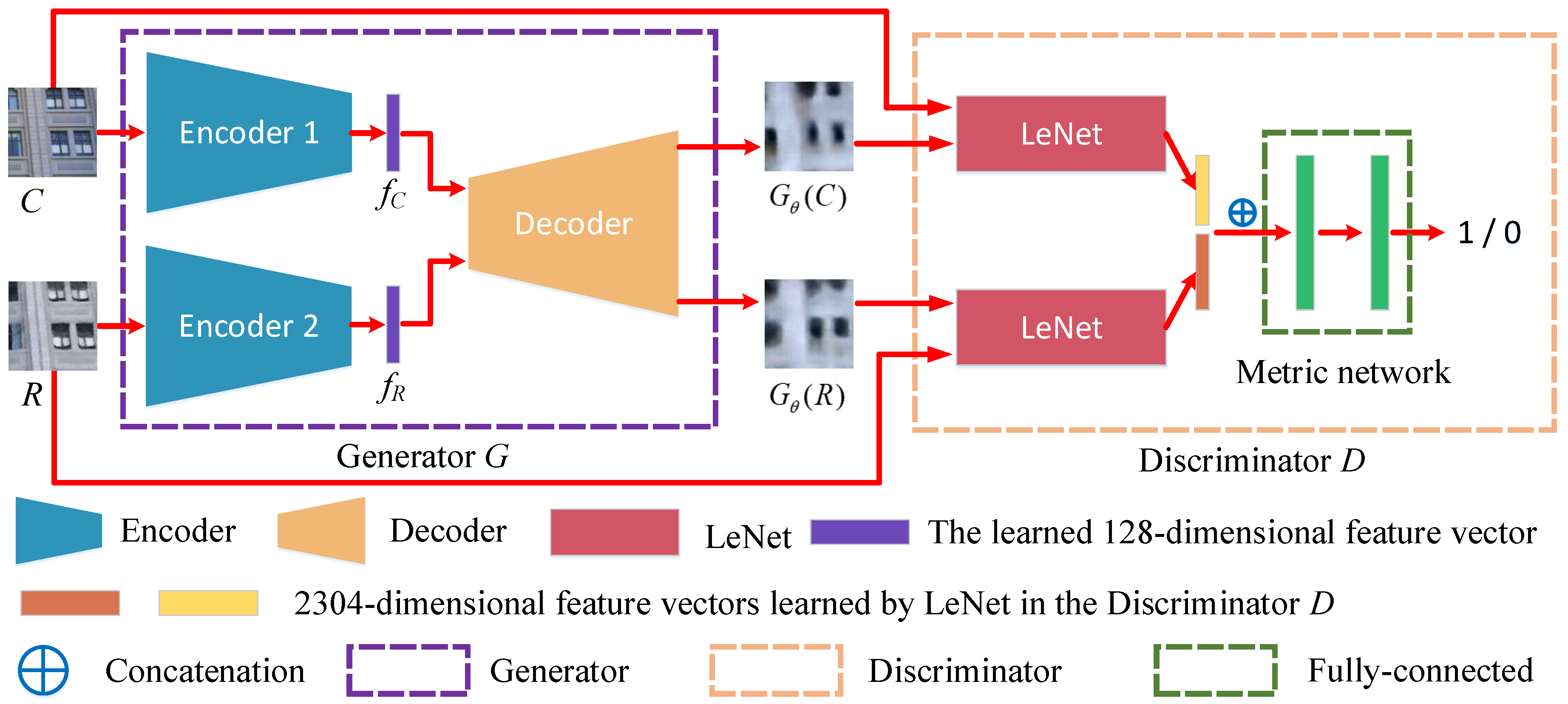
49]. There are two parts to GAN. One is the generative network (generator); the other is the discriminative network (discriminator). Typically, the adversarial strategy of GAN is that the generative network learns a mapper from a latent space to a data distribution of interest, while the discriminative network distinguishes candidates produced by the generator from the true data distribution. Thus, inspired by the above GANs approach, we propose AE-GAN-Net to learn the invariant feature descriptors for ground camera images and rendered images. AE-GAN-Net consists of two AutoEncoders with a shared decoder and one embedded GAN. The detailed framework of AE-GAN-Net is shown in
Figure 4.
AE-GAN-Net aims to use an adversarial strategy to encourage the paired images generated by the generator (if the inputs are matching paired cross-domain images) to be as similar as possible, and let the paired images generated by the generator (if the inputs are non-matching paired cross-domain images) be dissimilar. Then, we use the shared decoder to backwardly infer that the learned feature descriptors are invariant for the inputs, which are matching pairs of cross-domain images.
3.1. Network Structure
Furthermore, as shown in
Figure 4, AE-GAN-Net can be divided into two components: generator network
G and discriminator network
D. The descriptions of generator and discriminator are as follows:
Generator network G. Generator
G consists of two autoencoders with a shared decoder. The inputs are labeled raw paired cross-domain image patches whose sizes are resized to 256*256*3, and the outputs are 128-dimensional feature descriptor vectors learned by the encoders. In detail, two unshared encoders have the same structure: convolution layers with zero padding and max pooling layers without zero padding. Batch Normalization (BN) [
50] is used after each convolution; the non-linear activate function is SeLU [
51]. The structure of the encoder is as follows: C(32,5,2)-BN-SeLU-C(64,5,2)-BN-SeLU-P(3,2)-C(96,3,1)-BN-SeLU-C(256,3,1)-BN-SeLU-P(3,2)-C(384,3,1)-BN-SeLU-C(384,3,1)-BN-SeLU-C(256,3,1)-BN-SeLU-P(3,2)-C(128,7,1)-BN-SeLU, where C
is a convolution layer with
n filters of kernel size
having stride
s; P
is the max pooling layer of size
with stride
s.
For the shared decoder in generator G, we use transposed convolution to reconstruct the learned 128-dimensional feature descriptors as a 256*256*3 image. Before deconvolution (transposed convolution), we first map the 128-dimensional feature descriptor to a 1,024-dimensional vector by a fully connected layer. The detailed decoder structure is as follows: FC(128, 1024)-TC(128,4,2)-SeLU-TC(64,4,2)-SeLU-TC(32,4,2)-SeLU-TC(16,4,2)-SeLU-TC(8,4,2)-SeLU-TC(4,4,2)-SeLU-TC(3,4,2)-Sigmoid, where FC represents the input p-dimensional feature vector map to q-dimensional feature vector through a fully connected layer; TC represents the transposed convolution with n output channels of size and stride s.
Discriminator network D. The input for discriminator
D includes two kinds of cross-domain image pair patches with the size of 256*256*3. One kind of the patches is the same as the input (labeled raw paired cross-domain image patches) for generator
G; the other kind of patches is the labeled paired cross-domain image patches generated by generator
G (these labels are the same as the input of generator
G). The difference between the two input images is that one is the original image data and the other is the generated image data. These two kinds of image data enrich the input of discriminator
D, so that discriminator
D would have stronger discriminating ability after training. The output of discriminator
D is a binary value. If the input image patch pairs match, the output of discriminator
D is 1; otherwise, the output of discriminator
D is 0. In detail, discriminator
D consists of a Siamese network with a metric network. LeNet [
52] is used for the two branches, whose weights are not shared. Because the outputs of the two branches are feature maps, we stretch the feature maps into two one-dimensional vectors (2304-dimensional); then, we concatenate the two vectors into one vector (4608-dimensional) and feed it into a metric network of two fully connected layers, whose output channels are 1024 and 1. The non-linear activate functions for the first fully connected layer and the last fully connected layer are ReLU and Sigmoid, respectively.
In summary, the training data for AE-GAN-Net are a set of cross-domain image patch pairs with associated labels, and the AE-GAN-Net outputs 128-dimensional robust feature descriptors learned by the encoder in generator G.
3.2. Loss Function
To learn invariant feature descriptors for cross-domain images, a domain-consistent loss, which consists of content, feature consistency, and adversarial losses, is proposed to optimize AE-GAN-Net. We follow the optimization approach in GAN training for this minimax two player game setting and consider the following optimization problem that characterizes the interplay between generator
G and discriminator
D:
where
is the Expectation;
are the inputs of labeled raw paired image patches;
C is the ground camera image patches;
R is the rendered image patches;
is a distribution over
,
is a distribution over
C and
is a distribution over
R;
G and
D are the generator and discriminator, respectively;
and
are the parameters of
G and
D, respectively;
is a trade-off constant;
and
are the content loss and feature consistency loss which are defined by Equations (
4) and (
5), respectively.
In detail, to learn a generator distribution over data , the generator builds a mapping function from the prior noise distribution and to the data space as and , and the discriminator, , outputs a single scalar representing the probability that came from training data rather than . G and D are both trained simultaneously: we adjust parameters for G to minimize , and adjust parameters for D to minimize , as if they are following the two-player min-max game with value function .
Content loss. To extract the common features for the matching image patch pairs of ground camera images and rendered images, the pixel-wise Mean Squared Error (MSE) loss is used to minimize the two AutoEncoders with the shared decoder for the input of
C and
R:
where the size of the fed image patches is
,
N is the channel of the image, and
and
are image patches generated by shared decoder in generator
G. Thus, the total content loss is
Feature consistency loss. Our goal is to learn invariant feature descriptors for the cross-domain images. Thus, we use the following intuitive margin-based contrastive loss to constrain the feature descriptors of the labeled image patch pairs (To reflect patch similarity, Euclidean distance is used for the feature descriptors):
where
l is the label of the paired cross-domain image patches (if matched,
; otherwise,
);
is the Euclidean distance between feature descriptors
and
(learned by the encoders in generator
G) of
C and
R, respectively. Such feature consistency loss encourages the feature descriptors of matching pairs to be close and non-matching pairs to be separated by a distance of at least a margin
m.
Specifically, non-matching cross-domain image patch pairs contribute to the margin-based contrastive loss only if their feature distance is smaller than the margin
m. Equation (
5) encourages the matching cross-domain image patches to be close in the feature space, and punishes the non-matching cross-domain image patches that are margin
m away. As seen from the second part of Equation (
5), the non-matching pairs with the feature distance larger than margin
m will not contribute to margin-based contrastive loss. In fact, if the margin
m is set too small, the feature consistency loss will be optimized only over the set of matching pairs; on the contrary, a larger margin
m hampers learning. In our experiment, we set margin
m to 0.01.
Adversarial loss. We describe the adversarial loss with the training strategy of the generator and the discriminator. Details are as follows:
Discriminator D aims to discriminate correctly the input paired cross-domain image patches, whether or not they match. It should be noted that the input paired image patches contain labeled raw pairs of cross-domain image patches (inputs of AE-GAN-Net) and the labeled pairs of image patches generated by generator G (the labels are the same to the inputs of AE-GAN-Net). These two kinds of paired cross-domain image patches not only enable the discriminator D to discriminate raw inputs, but also be valid for the image patch pairs generated by generator G. Essentially, this is a data augmentation mode, which enhances discriminator D with stronger discriminating capability.
Specifically, we minimize the Binary Cross Entropy (BCE) [
53] between the decisions of discriminator
D and the label (matching or non-matching). Concretely, the loss functions for discriminator
D with raw paired image patches and generated paired image patches are defined as follows:
where label 1 denotes that the paired image patches
is a match; label 0 denotes the paired image patches
that are not a match. Thus, the loss function for discriminator
D is
where
denotes the inputs that are raw paired cross-domain image patches; and
denotes the inputs that are paired image patches generated by generator
G.
Generator
G tries to minimize the Binary Cross Entropy (BCE) loss between the decision made by discriminator
D and generate more realistic matching or non-matching paired image patches so that discriminator
D becomes completely confused. Finally, the total loss used for training generator
G can be defined as the weighted sum of all the terms, as follows:
where
,
and
are the weights of BCE, feature and content losses, respectively.
The training strategy is performed in an alternating fashion. First, discriminator D is updated by taking a mini-batch of labeled raw paired cross-domain image patches and a mini-batch of generated paired image patches (the outputs of generator G). Second, generator G is updated by using the same mini-batch of labeled raw paired cross-domain image patches.
In summary, after AE-GAN-Net has been trained to converge, the paired image patches, which are generated by generator G from the matching raw paired cross-domain image patches, are still similar. For example, regarding the testing of paired matching cross-domain image patches , which are fed into a trained AE-GAN-Net, we obtain . Then, using the shared decoder, the learned feature descriptors of c and r are , demonstrating that the matching cross-domain image feature descriptors learned by AE-GAN-Net are invariant.
3.3. Training Strategy
We implemented AE-GAN-Net with PyTorch framework, and trained it with a Nvidia 2080 Ti GPU. AE-GAN-Net is trained with labeled paired image patches of ground camera images and rendered images, and the generator and discriminator are minimax in an alternating fashion. All weights in both the generator and the discriminator are initialized by Gaussian distribution of zero-mean and standard deviation of 0.05. Batch size is set at 20. Both discriminator and generator are trained with the Adam optimizer [
54], which is an extension to stochastic gradient descent. Initially, the learning rates for the generator and discriminator are set at 0.0001 and 0.0002, respectively, and they both decreased 5% after 3 epochs. The discriminator is optimized three times more frequently than the generators.
4. Experiments
4.1. Dataset
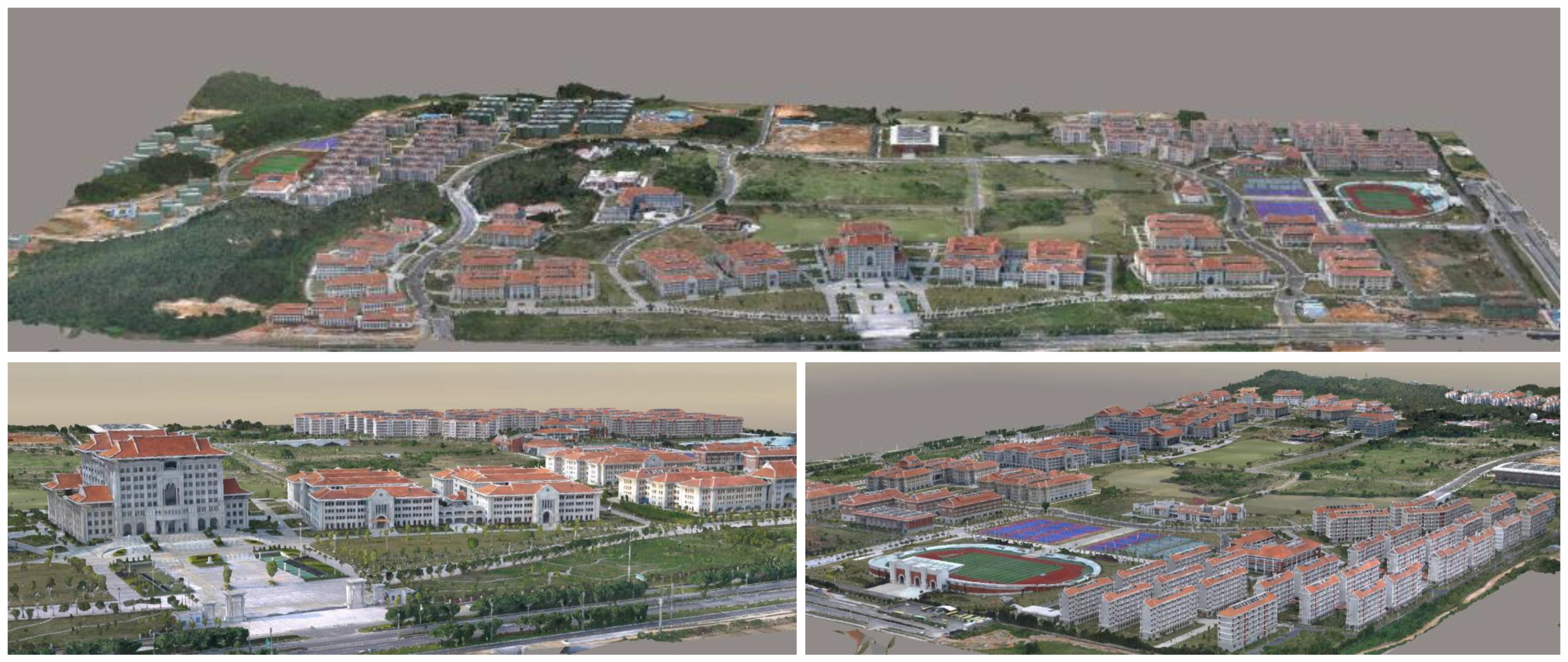
The cross-domain images adopted in this paper are the ground camera images and the corresponding rendered images, which were obtained from the Xiangan campus of Xiamen University, China, about 3-square-kilometer with 100+ buildings; 30,000+ vertical and oblique aerial images of the campus were captured by the UAVs. The 3D image-based point cloud was generated by the SfM algorithm, as shown in
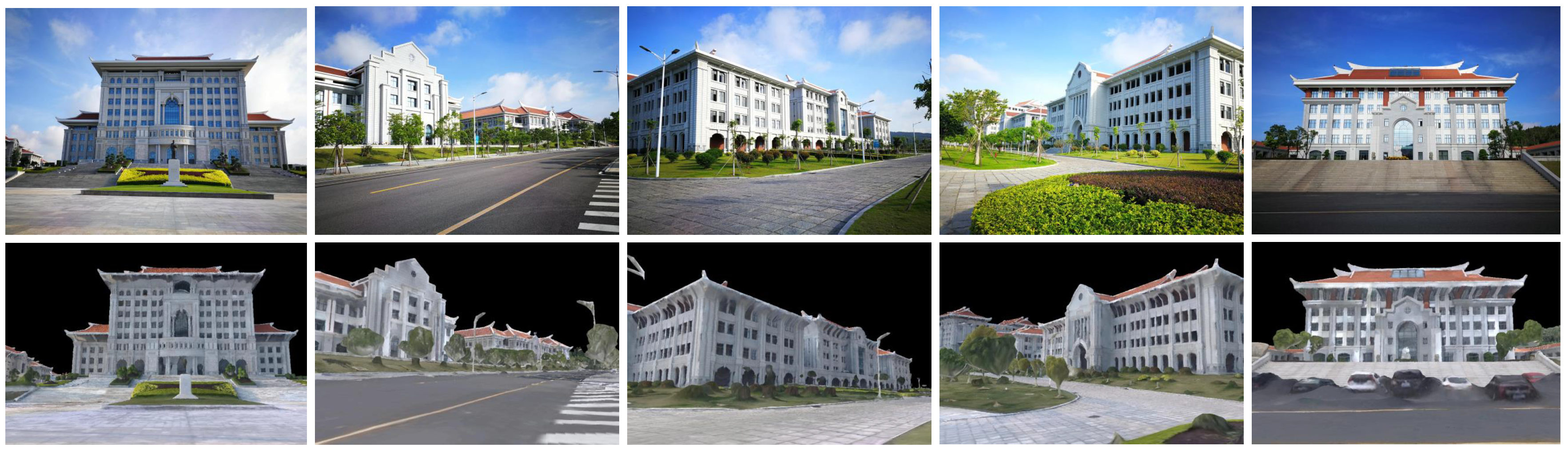
Figure 5. The resolution of this 3D image-based point cloud is about 2 cm. Then, we captured 10,000+ ground camera images by mobile phone (HUAWEI Mate 9 with Leica Dual Camera with a 12 MP RGB sensor and 20 MP monochrome sensor). During our tests, the GNSS error of HUAWEI Mate 9 mobile phone we used in the open outdoor is about 2 to 5 m. To acquire a camera pose, we set up the mobile phone on a handheld gimbal, which reduces the camera jitter, to capture images. In this way, we obtain synthetic images rendered from the 3D image-based point cloud, which are similar to the viewpoints of the corresponding ground camera images. Several samples of corresponding ground camera and rendered images are shown in
Figure 6.
The training data and the testing data, which do not intersect, are from different buildings. We use the paired cross-domain images of 90+ buildings to created the training data, and use the paired cross-domain images of 10 buildings to create the testing data. In addition, both the training and testing data are collected from different days when the weather is either sunny or cloudy. The ground camera images of the training data are captured by HUAWEI Mate 9; the ground camera images of testing data are captured from both HUAWEI Mata 9 and IPHONE 7 Plus.
To acquire the labeled samples, a semi-automated software was developed to select the corresponding points between each pair of the ground camera and the rendered images. Assuming that the transformation between these two corresponding cross-domain images is a perspective transformations; then, by randomly collecting several patches in the rendered images, the matching patches in the corresponding ground camera images are subsequently obtained. In detail, there are two parts for the semi-automated software. One is done manually; the other is done automatically. The part done manually selects at least 4 pairs of corresponding points on the ground camera image and rendered image to calculate the perspective transformation. The part done automatically randomly collects several rendered image patches in a rendered image, and then automatically maps these rendered image patches to the corresponding ground camera image through the above calculated perspective transformation to obtain the matching ground camera image patches.
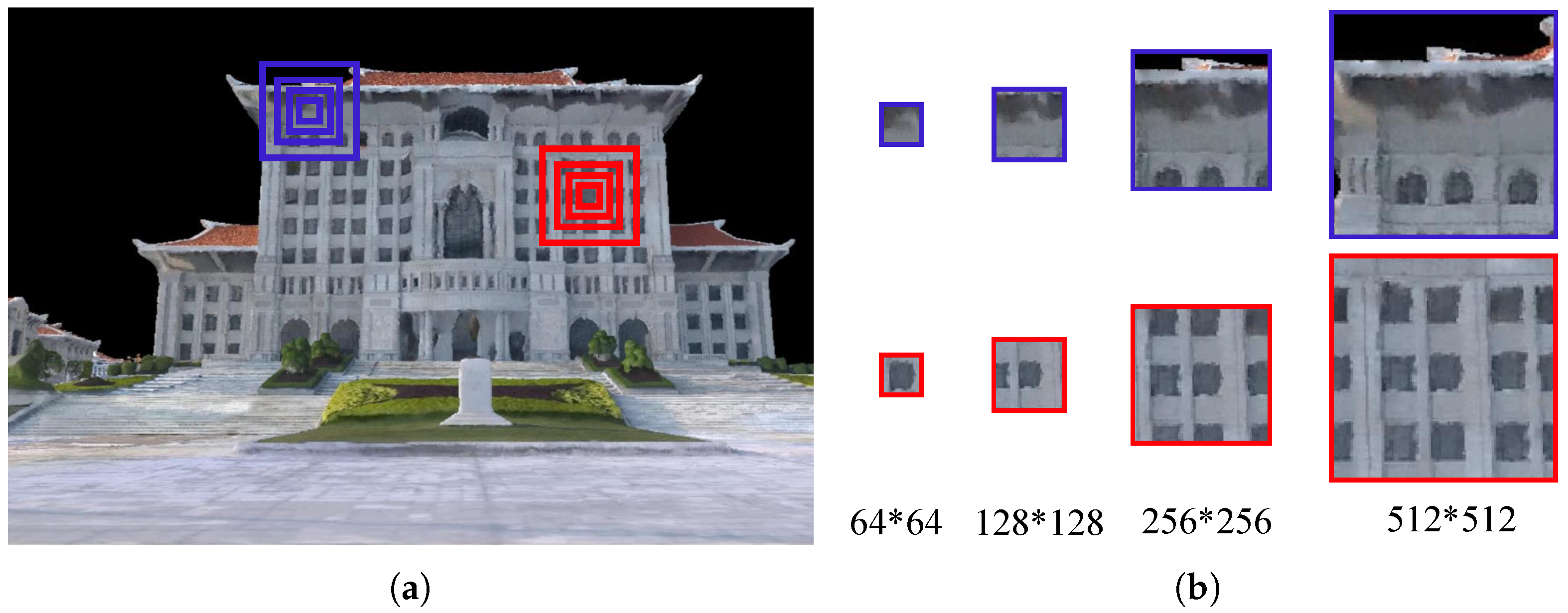
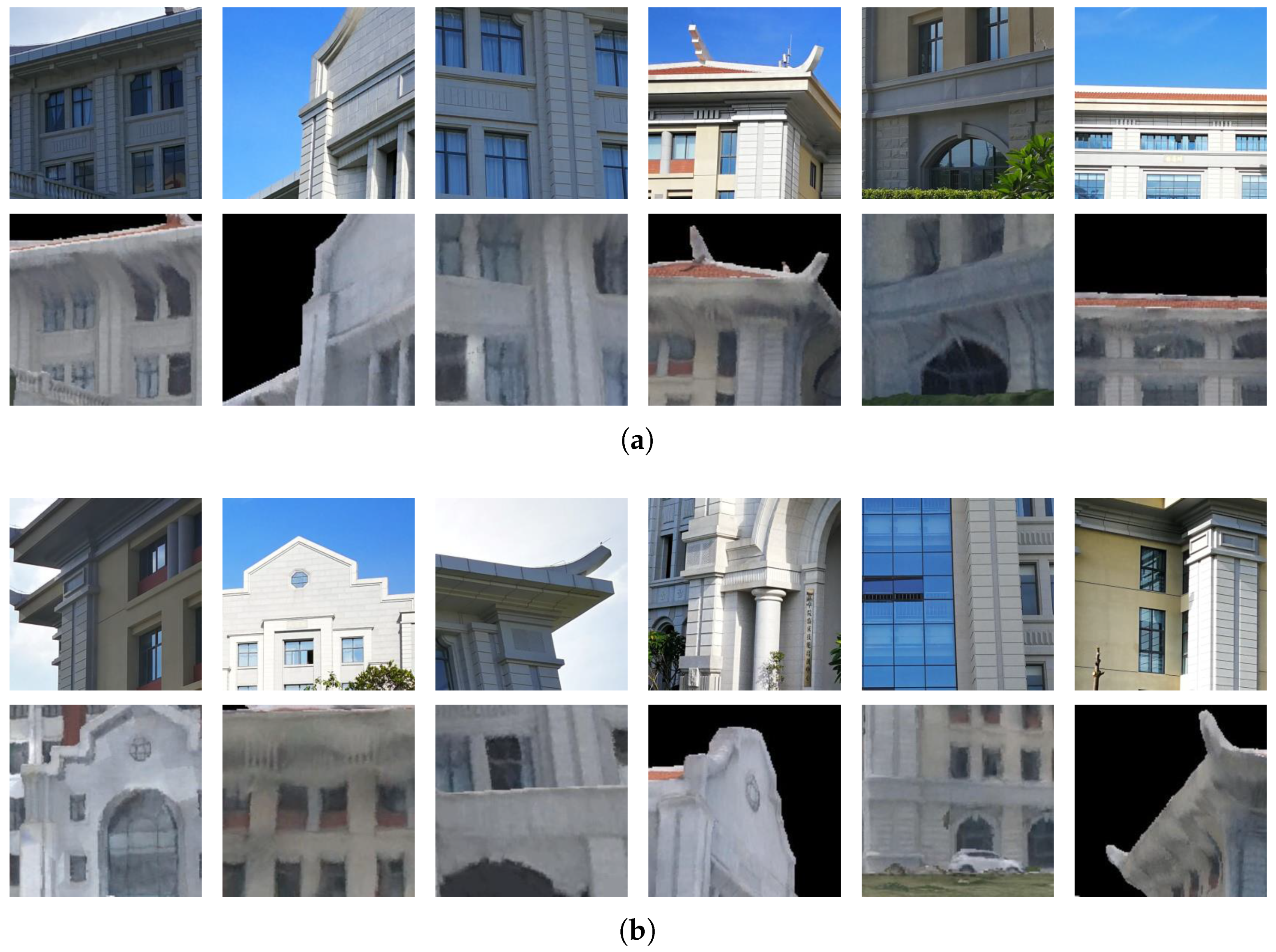
In addition, the size of the image patches must be carefully designed. If the size of a selected image patch is too small, the detailed information in the image patch will be limited; whereas, a large size patch becomes nearly a whole image, rather than a small image patch (Examples are illustrated in
Figure 7). Image patches have a high probability of being selected in the blurred regions of the rendered images (e.g., the position of the blue bounding boxes in
Figure 7a). It can be observed that if the size of the image patches is too small (e.g., 64*64 or 128*128), the patches will be in a completely blurred region, and the information loss will be very large (first row in
Figure 7b). Thus, small blurred image patches are worthless. Additionally, buildings with many very similar repeating structures, such as the windows shown within the red bounding boxes in
Figure 7a, lead to mismatches (second row in
Figure 7b). In practical applications, we should consider the spatial resolution. However, to create a large amount of training data (paired matching ground camera image patches and rendered image patches) more conveniently, we did not capture the buildings very close to the camera, as shown by the corresponding image pairs in
Figure 6. The reason is that if the distance is too short, buildings in the image will be large, and the size of the image patches cannot be well controlled. Therefore, the size of the image patches that we collected is between 256*256 and 512*512 pixels.
Based on the above considerations, 200,000+ matching and 200,000+ non-matching cross-domain image patch pairs were collected from the above 10,000+ corresponding ground camera and rendered images. The detailed distribution information of the 200,000+ matching cross-domain image patch pairs is describe as follows: First, all the synthetic images rendered from the 3D image-based point clouds are subject to huge distortions. Thus, in the training data, the 200,000+ rendered images are also distorted. Second, as described in the third paragraph of
Section 4.1, we set the size of the collected image patches to between 256 and 512 pixels. Thus, the number of image patches per size is about 700+ pairs. Third, because the position and orientation information obtained from the ground camera image are coarse, there is rotation bias between the ground camera images and corresponding rendered images. In addition, we only select the image pairs with a rotation bias of no more than 20 degrees, and vice versa. Several samples of collected cross-domain image patch pairs are shown in
Figure 8. These labeled cross-domain image patches are the training data for AE-GAN-Net and comparative neural networks.
4.2. Comparative Experiments
To demonstrate the superiority of AE-GAN-Net, we compared it with the existing mainstream feature descriptor learning neural networks. The TOP1 and TOP5 retrieval accuracy of the learned feature descriptors are used to measure performance. TOP1 retrieval is considered successful if the truly matched rendered image patch is ranked No.1. If the truly matched rendered image patch is retrieved in the first five ranked results, the TOP5 retrieval is considered successful. Results are listed in
Table 1. To ensure the fairness of the comparisons, 6000+ pairs of matching cross-domain image patches were additionally collected as a retrieval benchmark dataset. Specifically, the data in the retrieval benchmark dataset are not used in the training data. The distribution information of testing set is the same as that in training set, which is described in the above paragraph.
As shown in
Table 1, AE-GAN-Net achieves state-of-the-art retrieval performance for the learned feature descriptors on the established cross-domain image patch retrieval benchmark dataset, and shows significant improvement compared with the competing networks. DeepDesc [
22] and Siam_l2 [
44] are Siamese networks whose loss functions are constrained by Euclidean distance. DeepCD [
24] is an asymmetric Siamese network. To help optimize loss function, L2-Net [
23] introduces some constraints in the data sampling strategy. H-Net++ [
25] incorporates the AutoEncoder into the Siamese network. TNet [
27], DDSAT [
29] and DescNet [
30] use triplet loss with different data sampling strategies to learn the feature descriptors. DOAP [
28] extracts local feature descriptors optimized by average precision. It can be viewed that whether or not the feature descriptors are learned by simple Siamese networks, variant Siamese networks, or triplet networks, the learned feature descriptors are not robust for retrieval on ground camera images and rendered images.
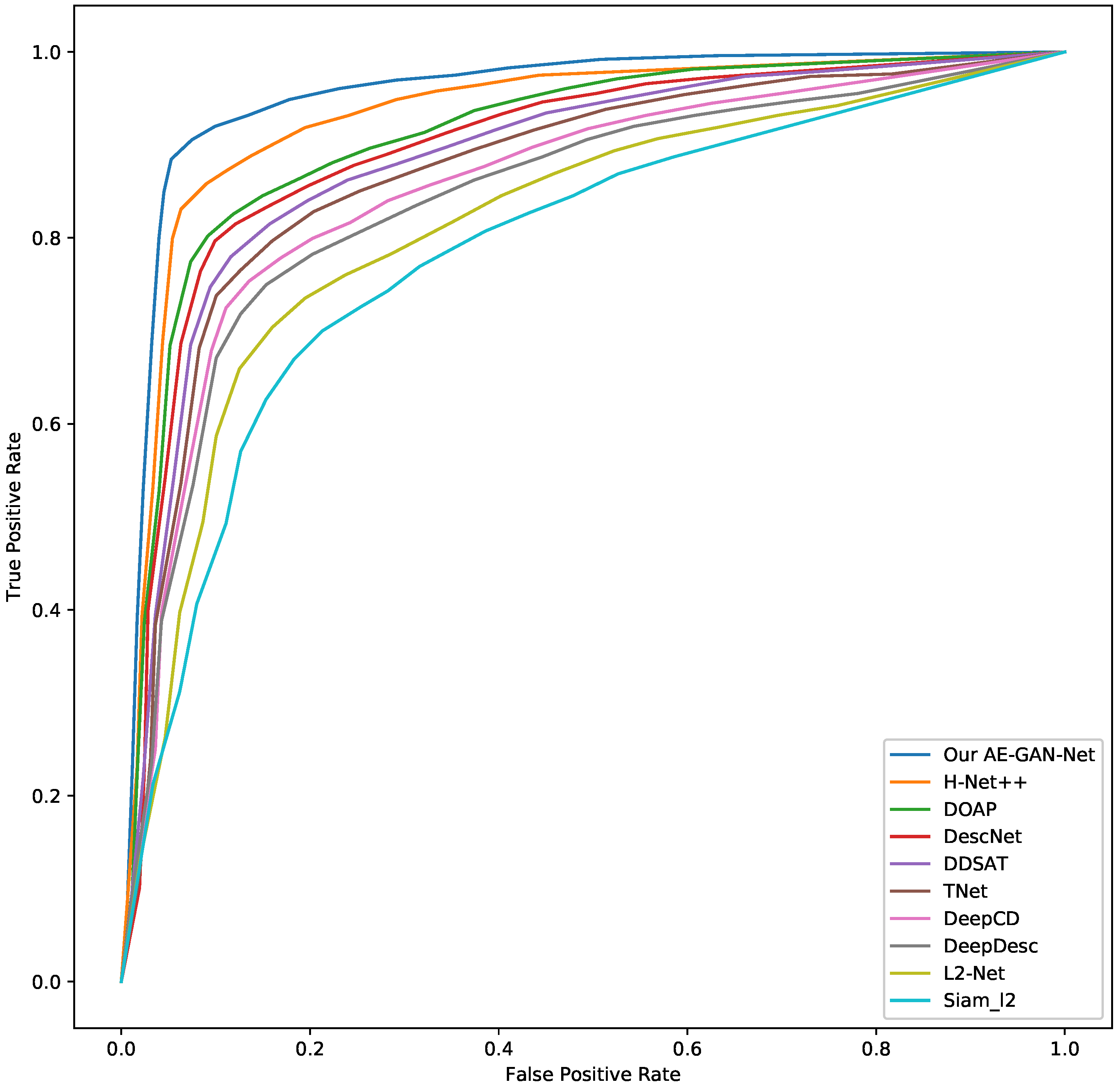
Moreover, we create another testing data, which are not used in the training data, to perform an accuracy assessment for our AE-GAN-Net and competing networks. The testing data is collected according to the following strategy: (1) Selecting 500 ground camera image patches, denoted as , ; (2) Selecting 500 rendered image patches, which are matched to , denoted as , ; (3) Selecting 500 rendered image patches, which are non-matched to , denoted as , . Thus, the testing data has 500 ground camera image patches and 1000 rendered image patches, which consists of 500 paired matching cross-domain image patches and 500 paired non-matching cross-domain image patches.
Then, using the above collected testing data, the detailed testing strategy is as follows: first, using the trained AE-GAN-Net to compute the feature descriptors of the above collected image patches; second, for each ground camera image patch in
, retrieving each ground camera image patch in
in the
and
to obtain the TOP1 retrieval result. Third, we draw the ROC curve based on the precision and recall, which is calculated by the TOP1 retrieval result. The ROC curves are shown in
Figure 9. From the ROC curves, it can be observed that our AE-GAN-Net has the best performance.
In addition, we also explored some ablation studies. First, to demonstrate the importance of the embedded GAN module, we removed GAN from AE-GAN-Net. However, it should be noted that without adversarial loss (GAN loss), AE-GAN-Net degenerates into a specific form of H-Net++ [
25], i.e., H-Net++ with a shared decoder. Results in
Table 1 show that AE-GAN-Net is 18.8% better than H-Net++. Second, for the weight of the adversarial loss (Equation (
9)), a small weight will lead to an inefficient constraint; whereas, a large weight will lead to mode-collapse. According to our experiments,
,
and
(Equation (
9)) are the most suitable weights for adversarial loss.
4.3. Invariance of the Learned Feature Descriptors
To demonstrate that the feature descriptors learned by AE-GAN-Net are invariant against distortion, viewpoint, spatial resolution, rotation and scaling, several experiments were performed with additionally collected datasets, as follows:
Distortion invariance. As described in
Section 1, the synthetic images rendered from 3D image-based point clouds are usually distorted and of low resolution. In contrast, the details of the ground camera images are fine. To extract the consistent feature descriptors for these two extremely different cross-domain images, we propose the AE-GAN-Net to learn invariant features for the ground camera images and rendered images. The experimental results in
Table 1 and
Figure 9 show that the feature descriptors learned by AE-GAN-Net are invariant. Thus, from these experimental results, we conclude that AE-GAN-Net can overcome the distortion of the rendered image to extract feature descriptors with distortion invariance, i.e., the feature descriptors of the cross-domain image patches learned by AE-GAN-Net are invariant against distortion.
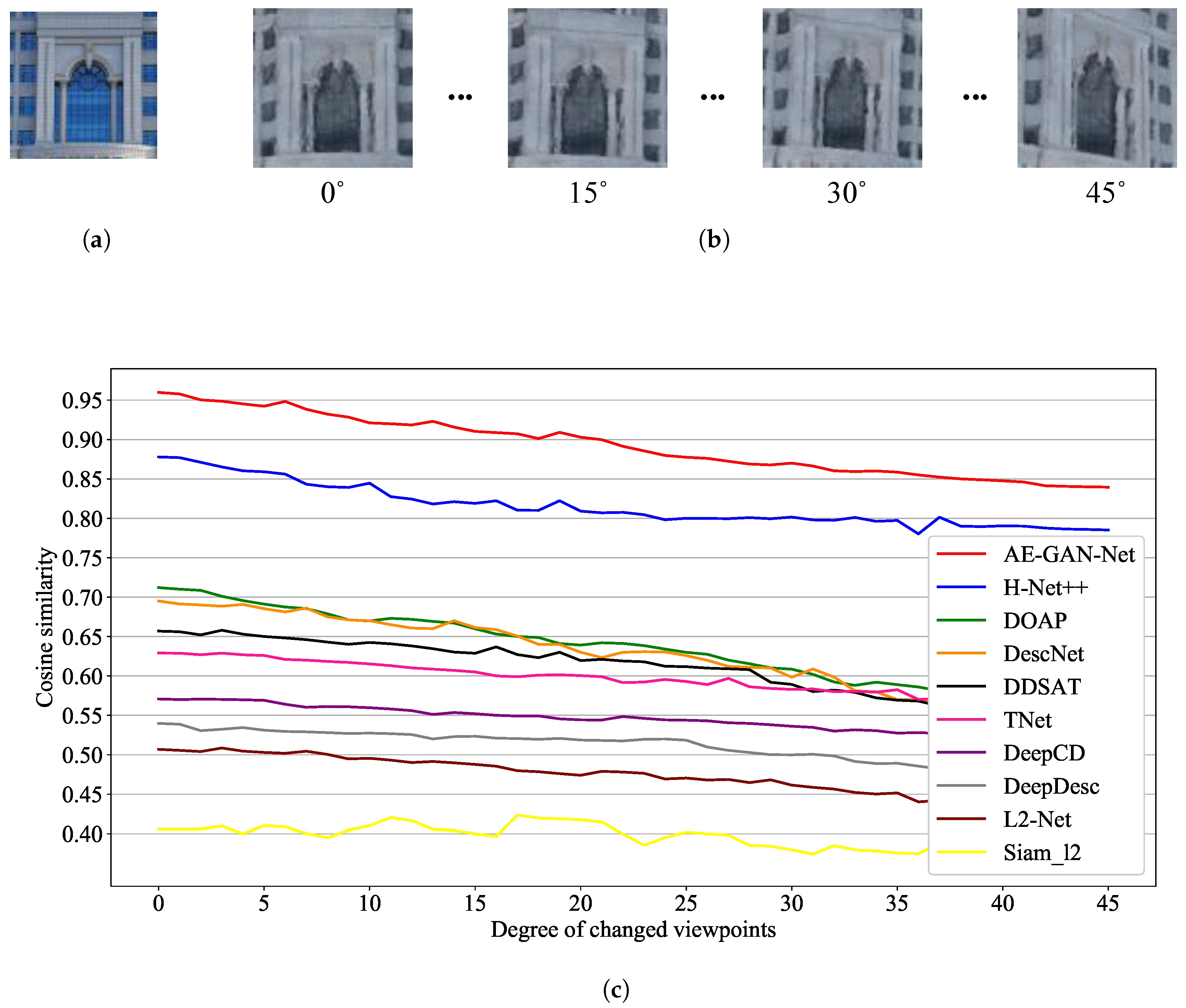
Viewpoint invariance. For the viewpoint invariance of the learned feature descriptors, we investigated cosine similarity for the learned feature descriptors on image patch pairs extracted from ground camera images and rendered images. First, we took a fixed viewpoint ground camera image patch (
Figure 10a) and the rendered image patches with different viewpoints from zero to 45 degrees (
Figure 10b). Second, we calculated the cosine similarity for the learned feature descriptor vectors from the above collected paired cross-domain image patches. In detail, the two vectors used to calculate the cosine similarity are the paired feature descriptors of the paired ground camera image patches and rendered image patches. The paired feature descriptor vectors are computed by the trained AE-GAN-Net, i.e., the two purple vectors in
Figure 4. Compared with other competing networks, the features extracted by AE-GAN-Net have the highest cosine similarity (the red line in
Figure 10c). Thus, the cosine similarity measurement verifies that the cross-domain image feature descriptors learned by AE-GAN-Net are invariant against viewpoint variations. In addition, the training data for the network training contains only paired cross-domain image patches at a similar viewpoint, and the paired cross-domain image patches with largely deviated viewpoints are not included in the training data. Therefore, all the curves in
Figure 10c show a decreasing trend.
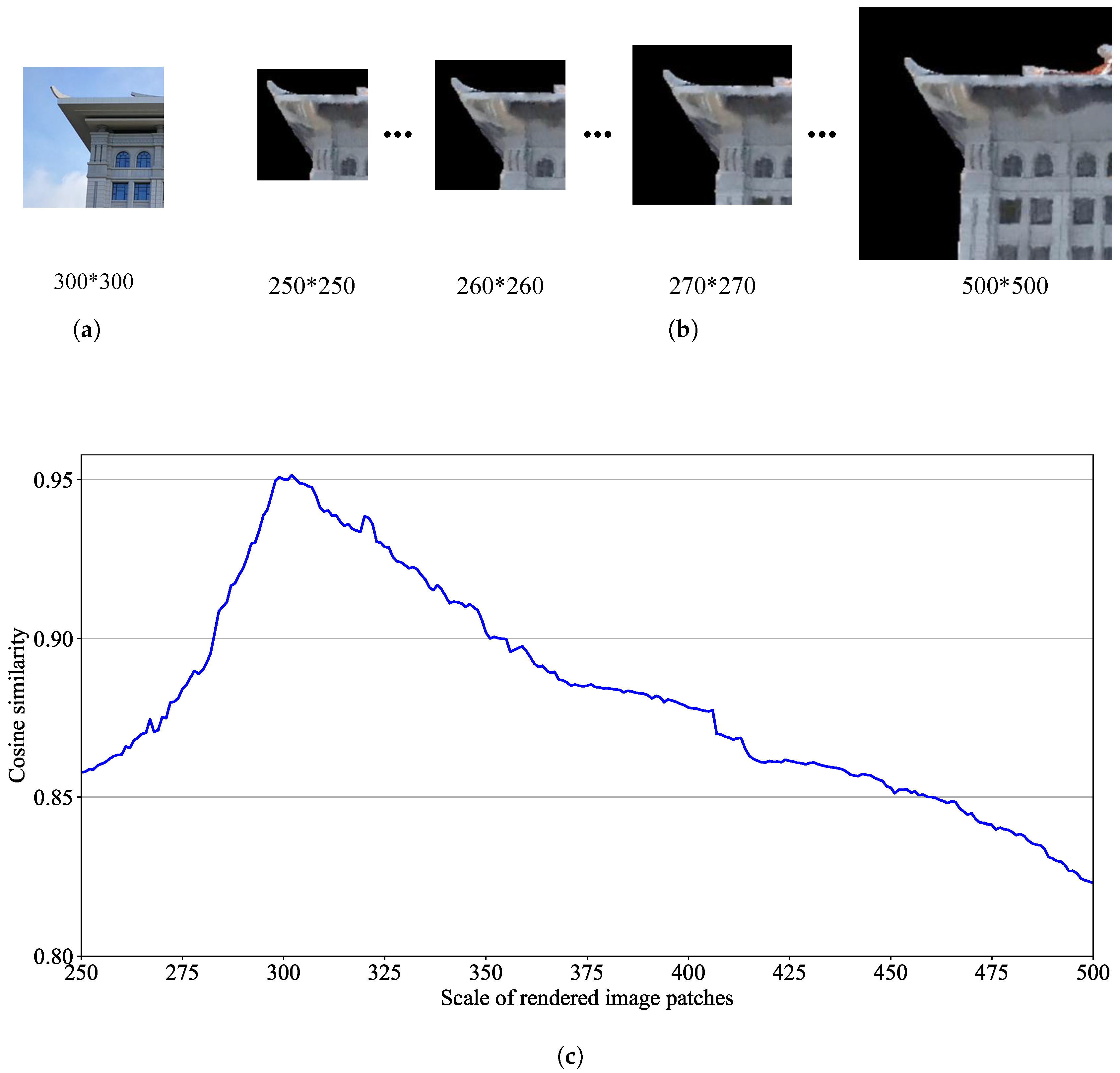
Spatial resolution and scale invariance. For the spatial resolution and scale invariance of the learned feature descriptors, we collected a multi-scale cross-domain paired patches dataset. We fixed a ground camera image patch with 300*300 pixels. Then, from the same viewpoint, we selected different sizes of rendered image patches (e.g., 251*251, 252*252, …, 500*500 pixels) for matching. The feature cosine similarity of these multi-size cross-domain patches were still maintained at a high level (between 0.8231 and 0.9508). The reason is that the size of the collected training data is between 256*256 and 512*512 pixels. Thus, AE-GAN-Net has learned the feature of various sizes of cross-domain image patches. This justifies that the features learned by AE-GAN-Net are invariant against spatial resolution and scale variations. An example of the cosine similarity of multi-size cross-domain patches is shown in
Figure 11.
Rotation invariance. To justify rotation invariance of the learned feature descriptors, we collected a rotational cross-domain paired patches dataset. We fixed a ground camera image patch and then obtained a total of 360 rendered patches by rotating the rendered images at different angles (degree by degree, counterclockwise selecting from the corresponding positions of the fixed ground camera image patch). The feature cosine similarity of these rotational cross-domain patches is still maintained at a high level (between 0.8701 and 0.9613). There is an inherent bias between the collected corresponding cross-domain images caused by the positioning error, including the viewpoints and positional bias, which cause the corresponding cross-domain images to have rotational deviation. Thus, the training data also contains the cross-domain image patch pairs with rotation offset. An example of the cosine similarity of rotational cross-domain patches is shown in
Figure 12.
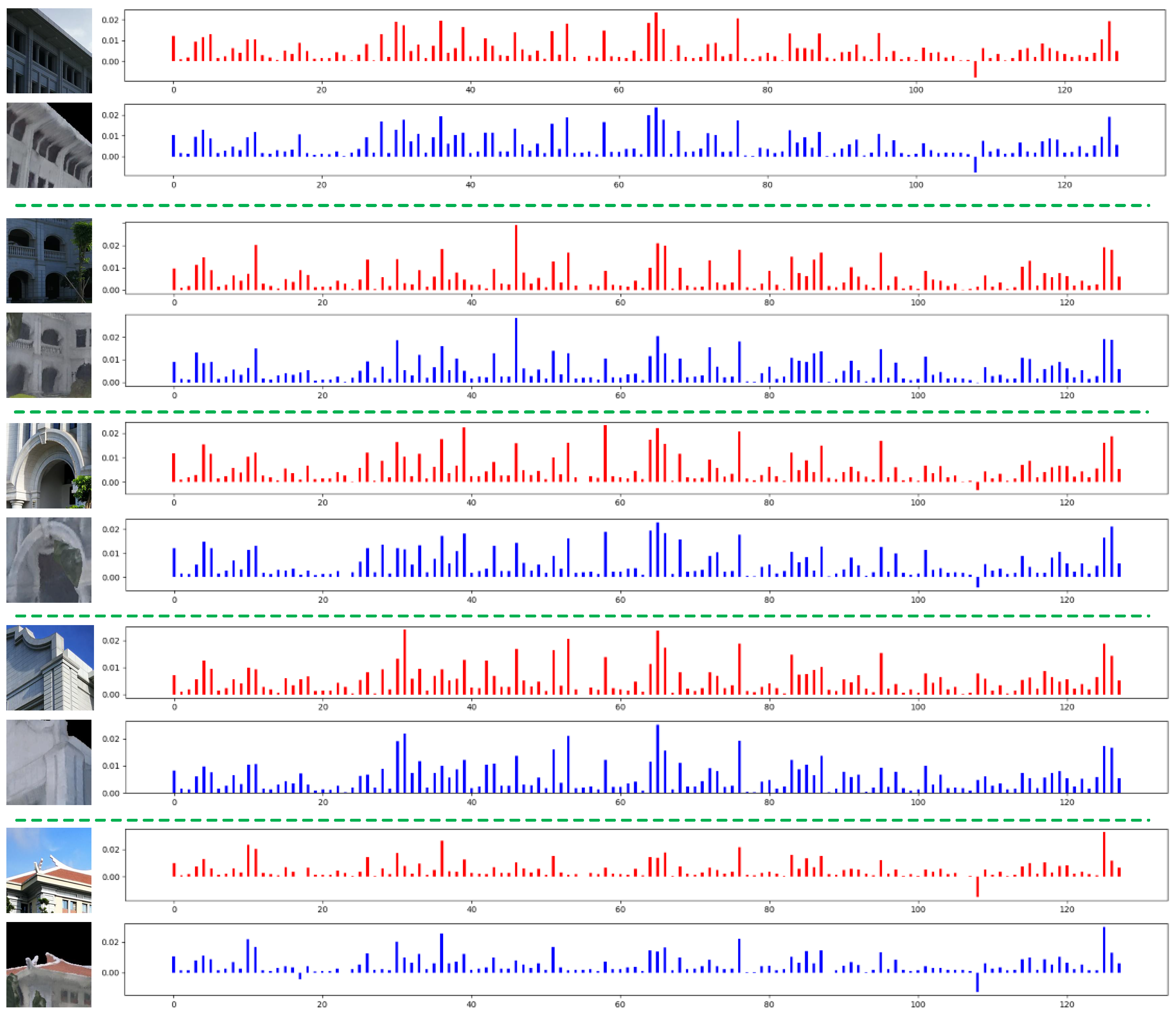
In addition, to better intuitively demonstrate the invariance of the feature descriptors learned by proposed AE-GAN-Net, we visualize the feature histogram of the learned feature descriptors in
Figure 13. The content shown in the histogram is the 128-dimensional feature descriptor vector learned by AE-GAN-Net. In the histogram, the
x-axis is the dimension of the feature vector, and the
y-axis is the value of the learned 128-dimensional feature descriptor vector. It can be observed that the feature distribution of each pair of matching cross-domain image patches is consistent, and the values of each dimension are similar. Thus, from the visualization of the similarity of the features, we conclude that the feature descriptors learned by AE-GAN-Net are invariant.
Note that the embedded GAN module in AE-GAN-Net is used to determine whether the cross-domain image patch pairs generated by the generator are similar. After training with a huge number of cross-domain image patch pairs, the strong performance of GAN in AE-GAN-Net enables it to decide if a pair of image patch pairs is a match or not. These image patch pairs may have distortions, various sizes, and rotation offsets. Thus, combined with the shared decoder and the constraint of feature loss, the feature descriptors learned by AE-GAN-Net are invariant.
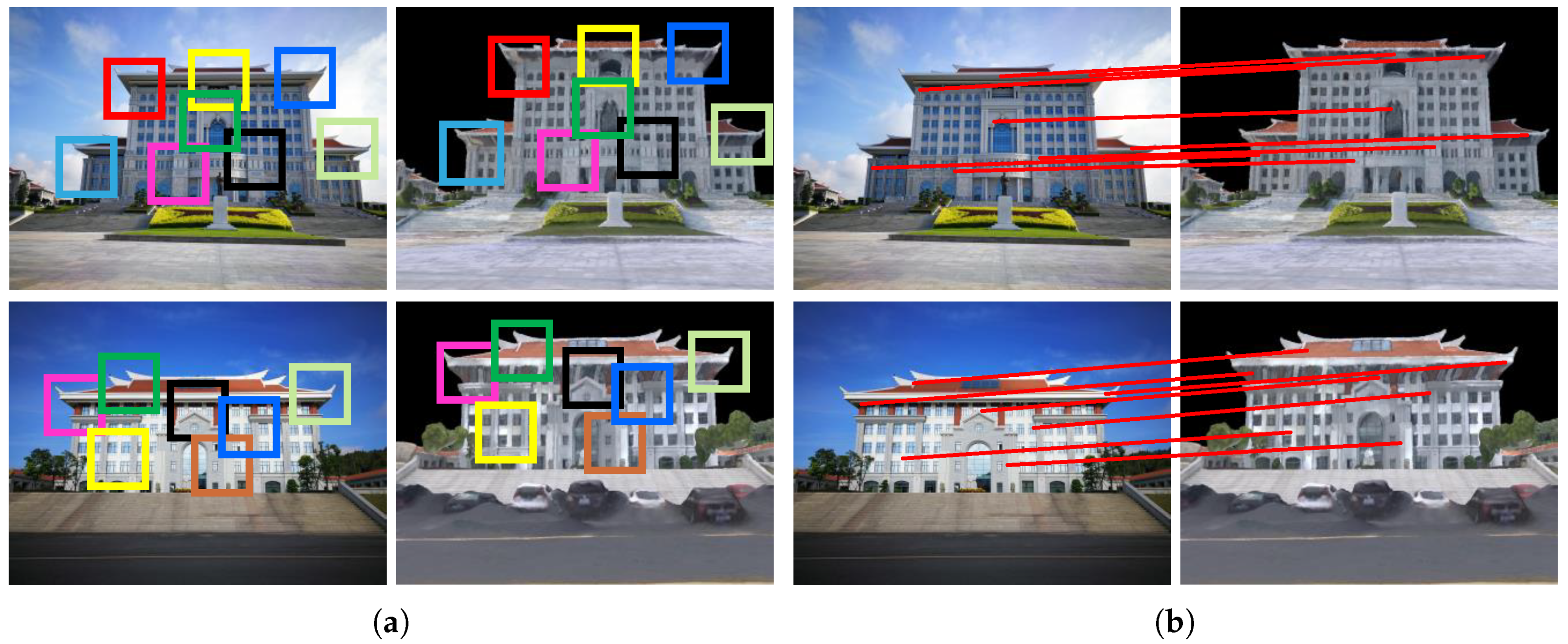
4.4. Image Matching and AR Applications
To match the ground camera images and the rendered images, the following four-step strategy is adopted: (1) Randomly select 2,000 points in each paired cross-domain images, and select 3 patches at each point (250*250, 375*375, 500*500 pixels); (2) Use the trained AE-GAN-Net to compute feature descriptors for the above selected image patches; (3) Apply the Nearest Neighbor Search (NNS) algorithm for retrieval and retain only the TOP1 retrieved results with cosine similarities greater than 0.9; (4) Apply RANSAC to filter mismatched results. In
Figure 14, we show the image patch matching results and center point connection of matching patches for the two pairs of cross-domain images in
Figure 3.
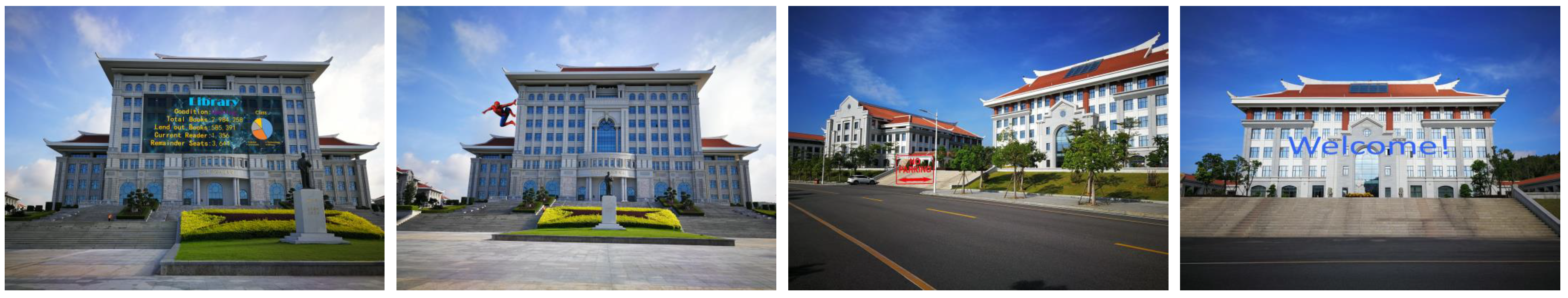
As shown in
Figure 15, the real-time library information, cartoon spider-man, NO PARKING sign and Welcome sign are registered into the open outdoor environments by the inferred spatial relationship. These AR applications demonstrate that the proposed virtual–real registration method is feasible for use in open and outdoor environments. However, the results have some limitations: the virtual objects have slight deformation after virtual–real registration, and there is a gap between virtual objects and targets (e.g., the gap between the cartoon spider-man and the building in
Figure 15).
5. Discussion and Analysis
Advantage of network framework. The framework of AE-GAN-Net consists of an AutoEncoder and GAN. For extracting domain-specific information, the AutoEncoder is more effective than CNN-based Siamese and triplet networks. The embedded GAN is used to constrain the generated image pairs; if the raw inputs are matching paired cross-domain images, the generated image pairs are similar, and vice versa. Thus, the embedded GAN improves the preservation of information in the feature encoder section. With the shared decoder, this constraint mechanism enables AE-GAN-Net to learn essential domain-consistent feature descriptors for ground camera and rendered images in dynamic balancing.
Effectiveness of domain-consistent loss. The content loss is used to reconstruct the generated images similar to the input images; the feature consistency loss is an intuitive loss, which constrains the feature descriptors unified in Euclidean space. Importantly, the adversarial loss makes the parameters of AE-GAN-Net update in an alternating fashion. This mechanism preserves the image content representation and balance feature descriptors consistency for ground camera images and rendered images.
Benefit of the discriminator. The training data for the discriminator contains not only raw labeled paired cross-domain images, but also the image pairs generated by the generator. These two kinds of image data make the discriminator more discriminative. Therefore, if the inputs are matching cross-domain images, the stronger discriminator will help the generator generate more similar image pairs.
In addition, there is a problem regarding lens distortion. In fact, deep learning networks can eliminate the influence of lens distortion when learning the features from images. For example, ResNet [
55] and Faster R-CNN [
56] are trained with ImageNet [
57] for image classification, recognition, and detection. The training data contains a large amount of image data from different cameras with different lens distortions. However, the above deep learning networks still learn robust features for their tasks without being affected by the lens distortion. Thus, the lens distortion is eliminated by deep learning networks, including our proposed AE-GAN-Net.
Although feature descriptors learned by AE-GAN-Net for ground camera images and rendered images are invariant, there are still some limitations. If the images have large occlusion and distortion, the learned feature descriptors will be meaningless and will result in failed matching results. In fact, image matching for very poor-quality cross-domain images often fails and sometimes beyond human capabilities for such tasks. In addition, we only focus on verifying the feasibility of our proposed virtual–real registration of AR in outdoor environments. Not considering the impact of the spatial resolution of the images is the drawback of this paper. Currently, our method cannot deal with the close-up images. In future work, we will try to solve this problem.
Moreover, rendered images rely heavily on positioning information (position and orientation) from the mobile phone. Thus, our proposed virtual–real registration approach of AR in outdoor environments is efficient and intuitive, but it is limited to open outdoor environments. For a dense building environment, more sensors may be needed to obtain accurate positioning.


 ,
, 


