Experimental Dynamic Impact Factor Assessment of Railway Bridges through a Radar Interferometer

 ,
,  ,
, 
Abstract
1. Introduction
2. Materials and Methods
2.1. The Railway Bridges
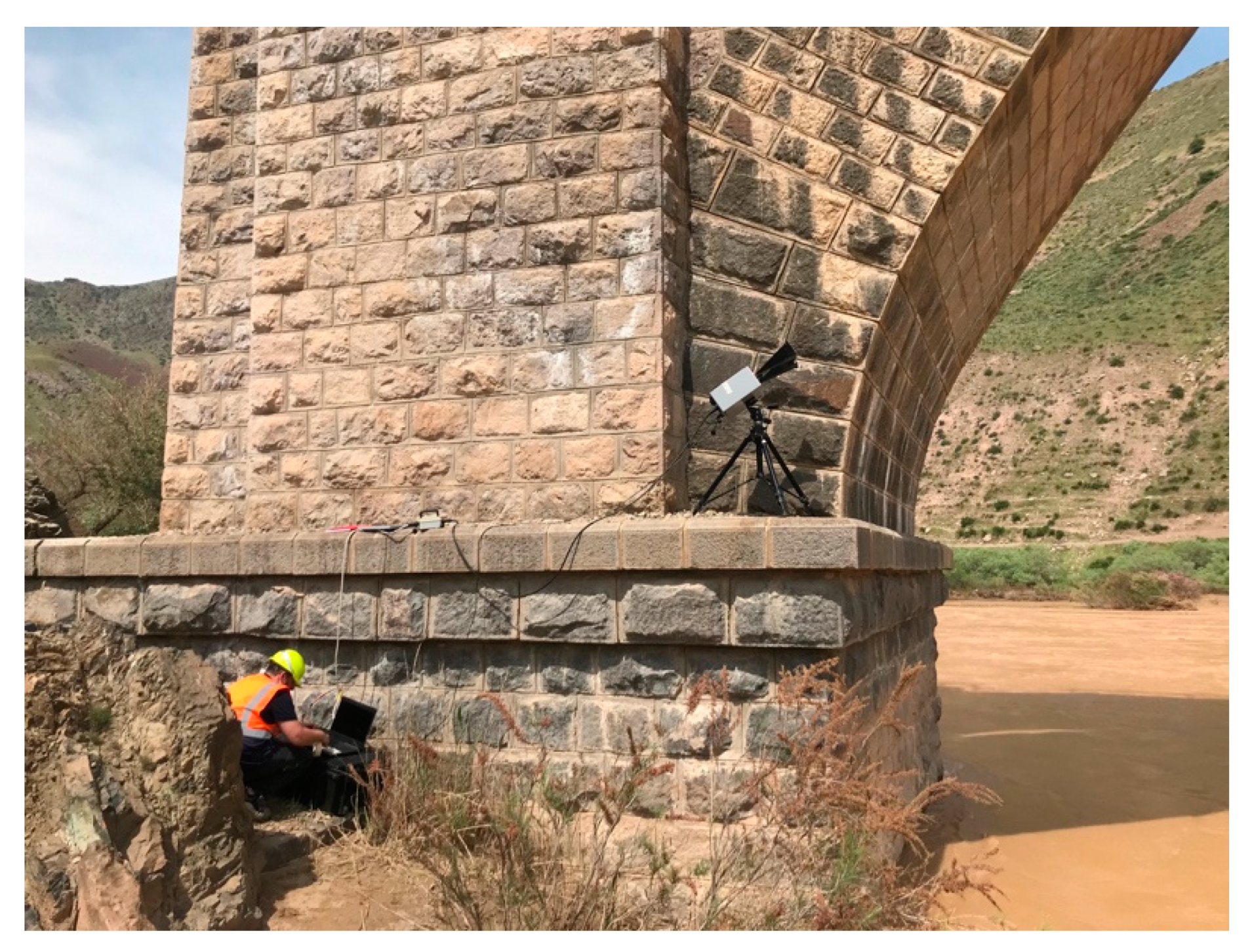
2.2. The Radar Equipment
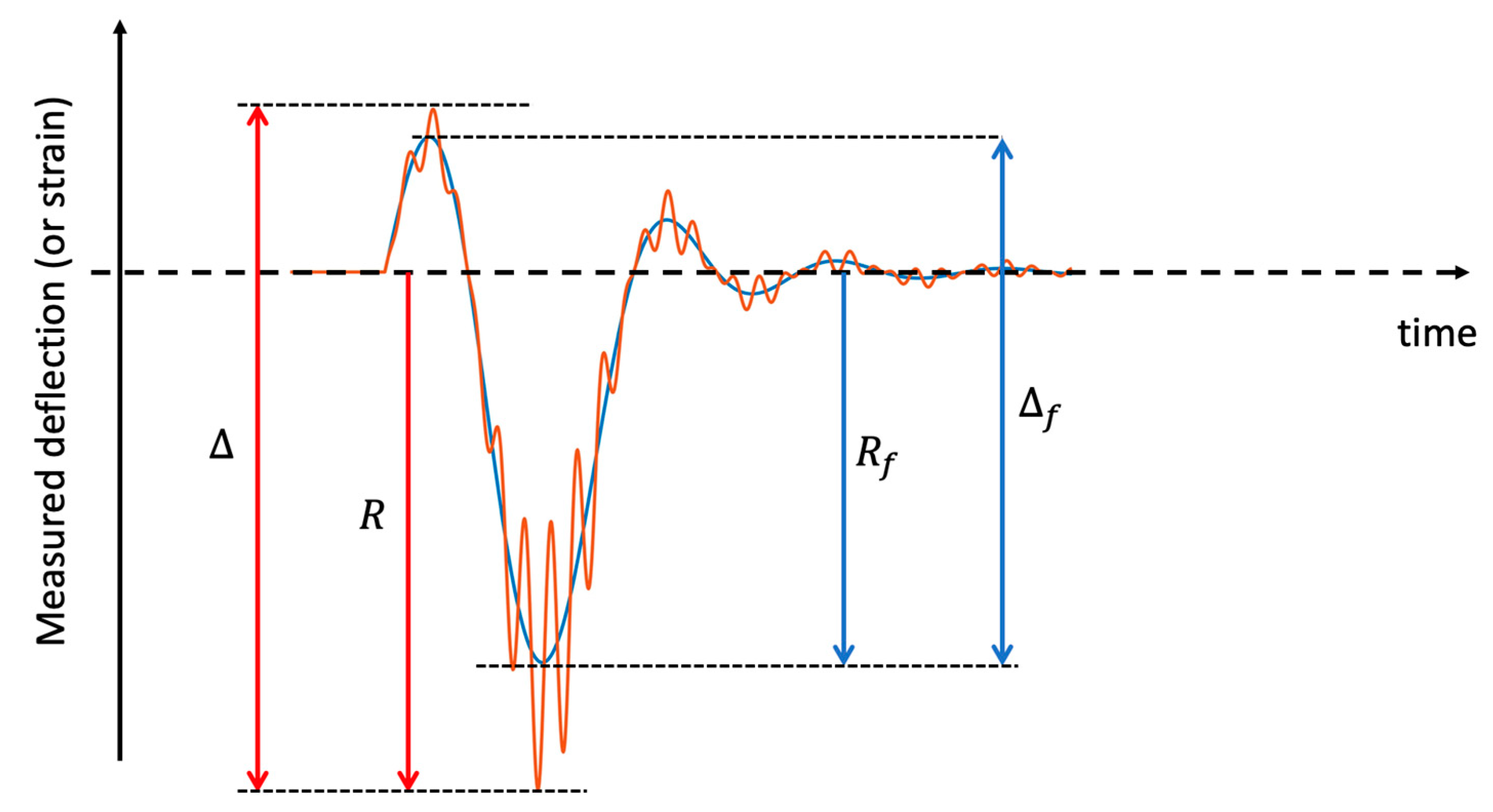
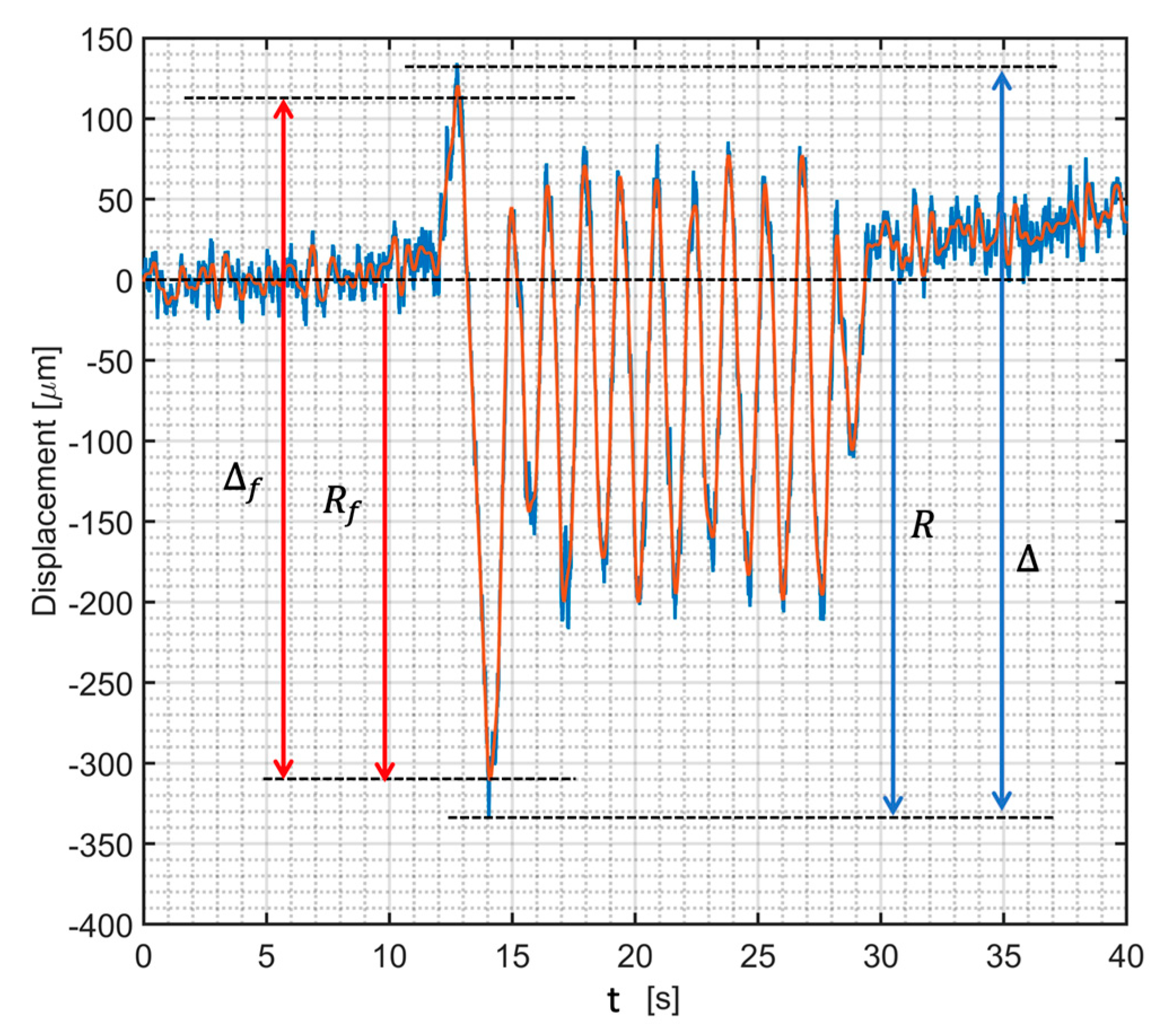
2.3. The Dynamic Impact Factor Definition
3. Results
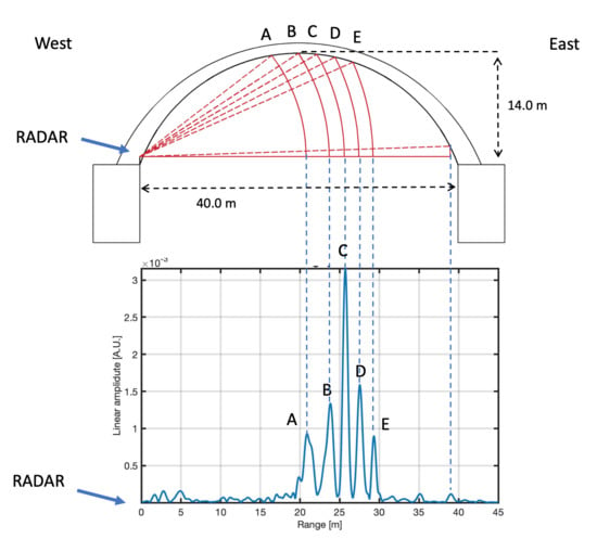
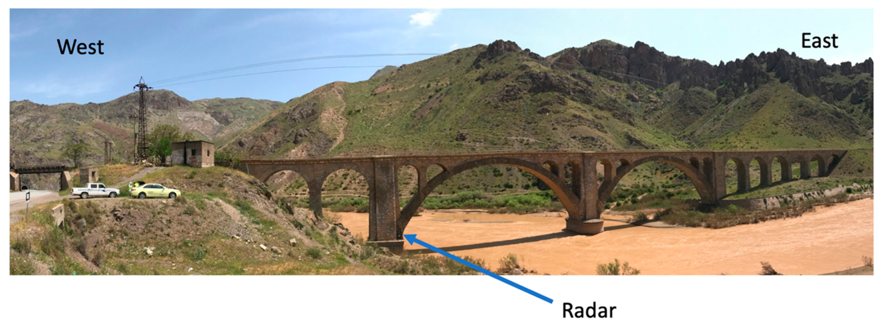
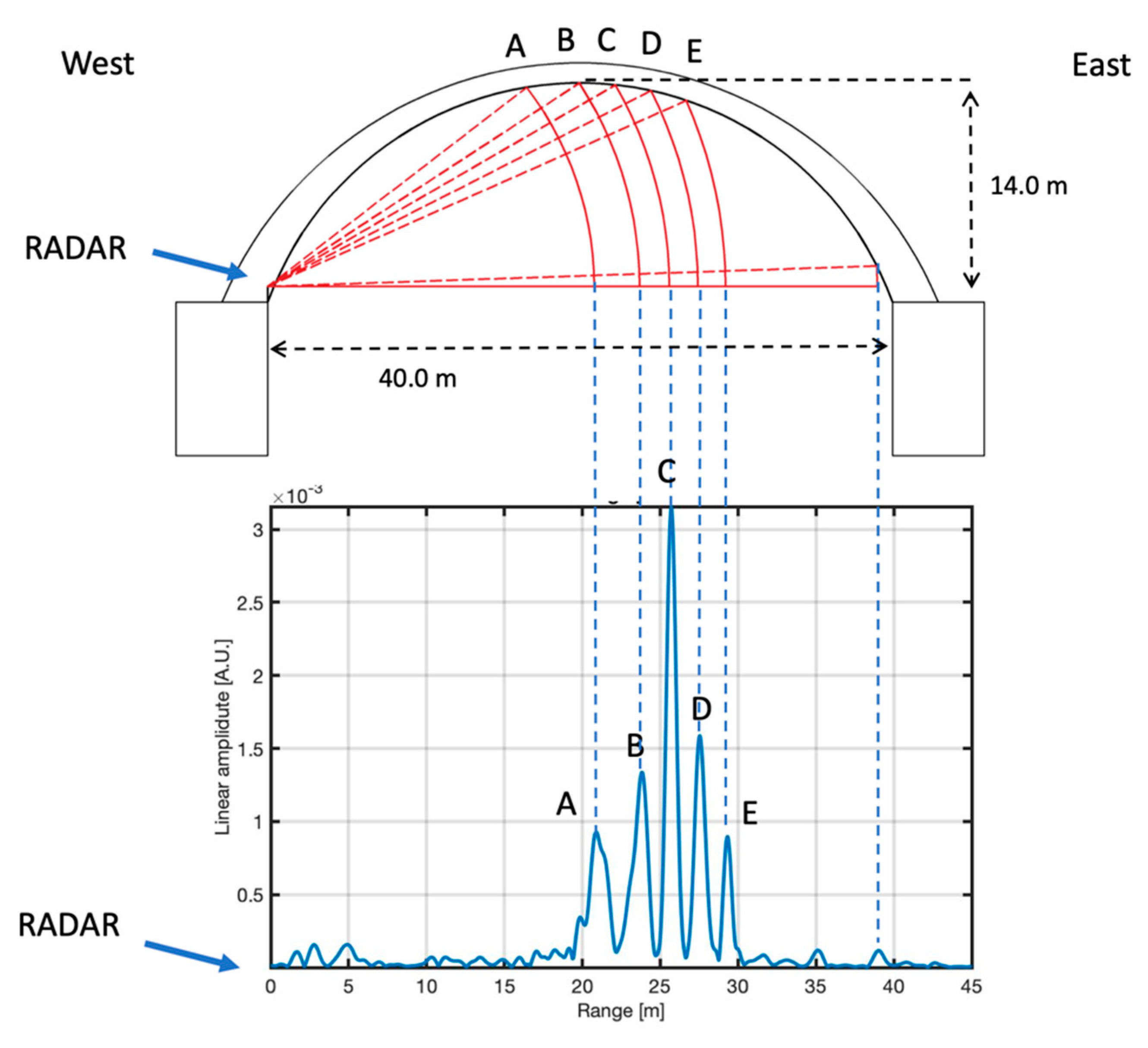
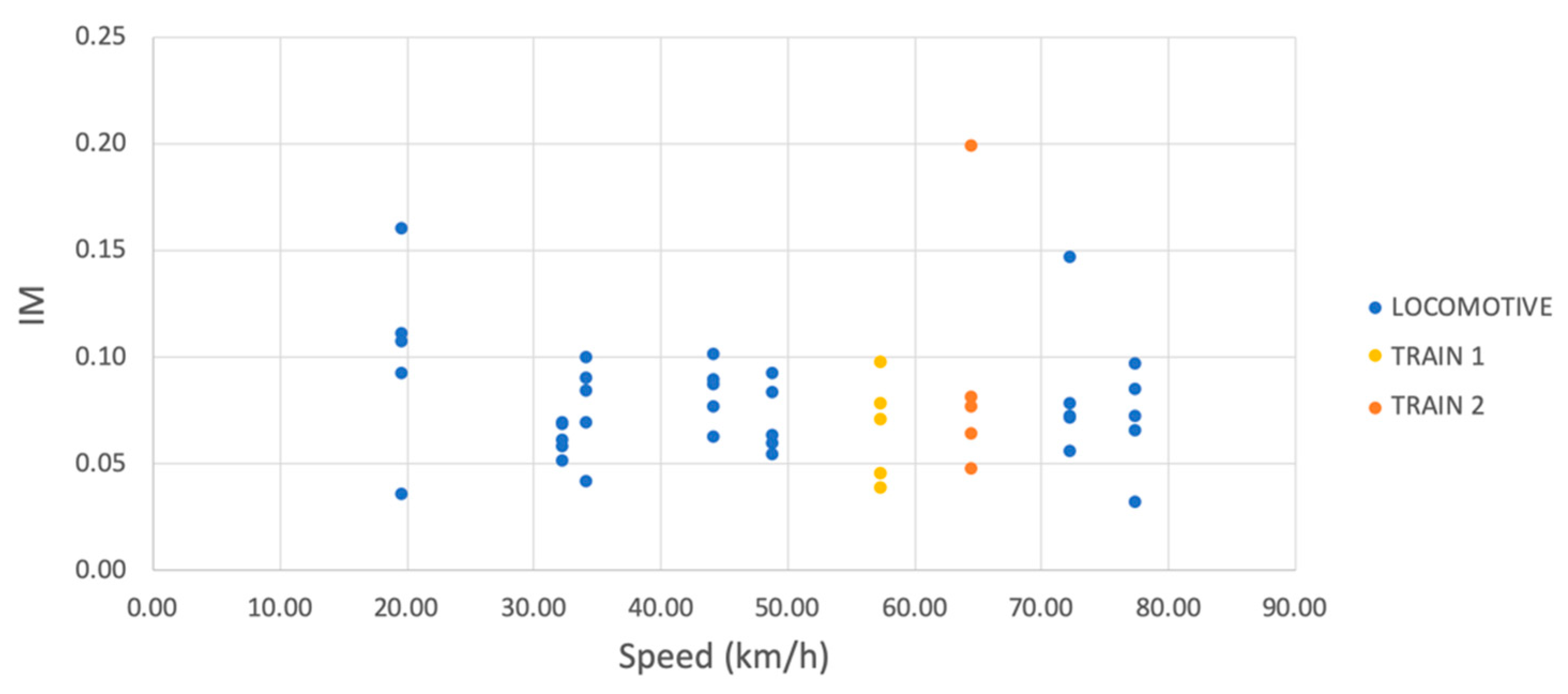
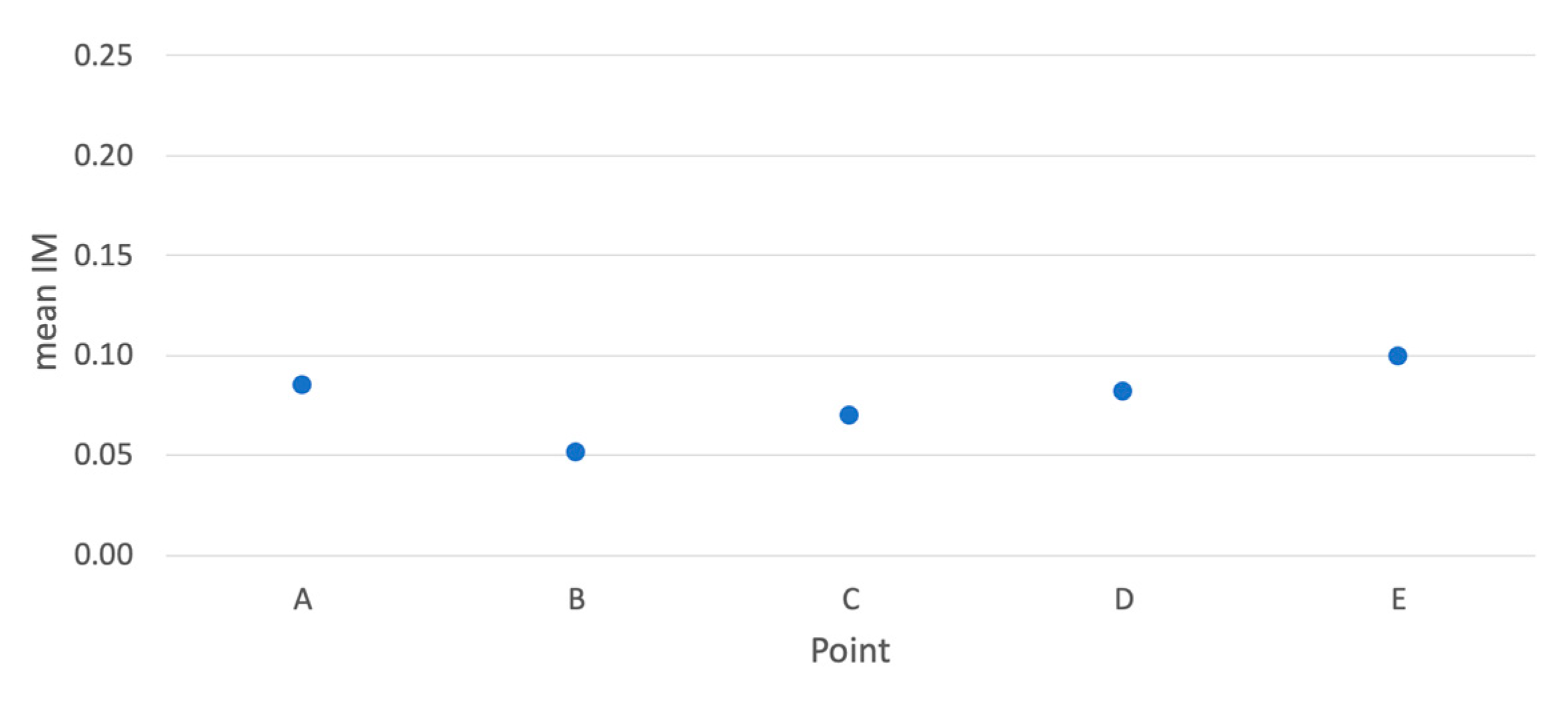
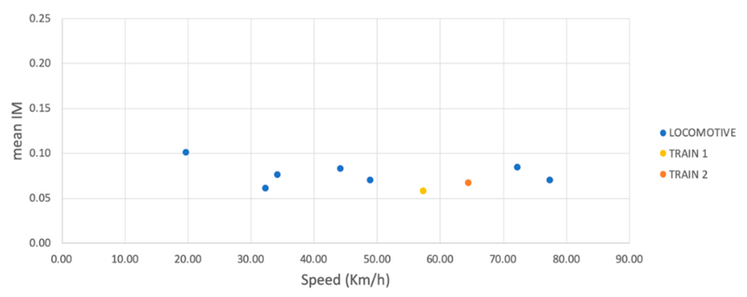
3.1. Veresk Bridge
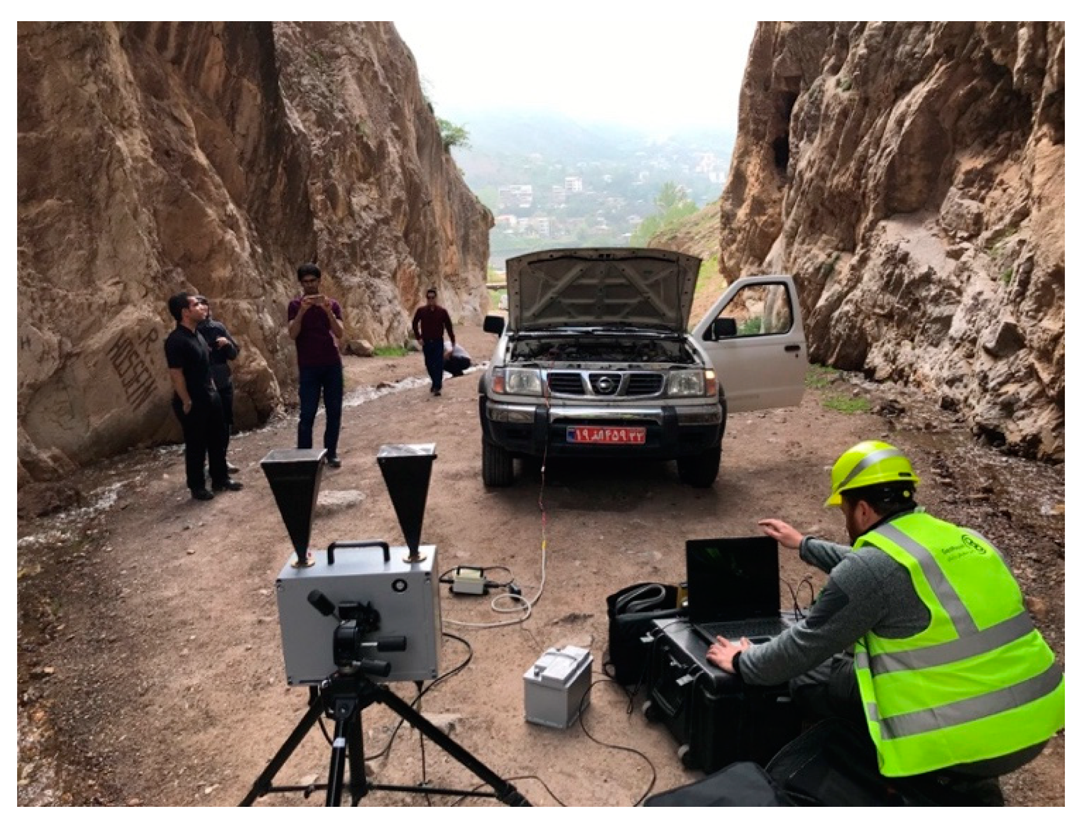
3.2. Kaflan-Kuh Bridge
4. Discussion
5. Conclusions
Author Contributions
Funding
Acknowledgments
Conflicts of Interest
References
- Deng, L.; Yu, Y.; Zou, Q.; Cai, C.S. State-of-the-art review of dynamic impact factors of highway bridges. J. Bridge Eng. 2015, 20, 04014080. [Google Scholar] [CrossRef]
- Paeglite, I.; Paeglitis, A. The Dynamic Amplification Factor of the Bridges in Latvia. Procedia Eng. 2013, 57, 851–858. [Google Scholar] [CrossRef]
- Ataei, S.; Miri, A. Investigating dynamic amplification factor of railway masonry arch bridges through dynamic load tests. Constr. Build. Mater. 2018, 183, 693–705. [Google Scholar] [CrossRef]
- Frýba, L. A rough assessment of railway bridges for high speed trains. Eng. Struct. 2001, 23, 548–556. [Google Scholar] [CrossRef]
- Xia, H.; Zhang, N. Dynamic analysis of railway bridge under high-speed trains. Comput. Struct. 2005, 83, 1891–1901. [Google Scholar] [CrossRef]
- Youliang, D.; Gaoxin, W. Evaluation of dynamic load factors for a high-speed railway truss arch bridge. Shock Vib. 2016, 2016, 5310769. [Google Scholar] [CrossRef]
- Flener, E.B.; Karoumi, R.; Sundquist, H. Field testing of a long-span arch steel culvert during backfilling and in service. Struct. Infrastruct. Eng. 2005, 1, 181–188. [Google Scholar] [CrossRef]
- Kwasniewski, L.; Wekezer, J.; Roufa, G.; Li, H.; Ducher, J.; Malachowski, J. Experimental evaluation of dynamic effects for a selected highway bridge. J. Perform. Constr. Facil. 2006, 20, 253–260. [Google Scholar] [CrossRef]
- Szurgott, P.; Wekezer, J.; Kwasniewski, L.; Siervogel, J.; Ansley, M. Experimental assessment of dynamic responses induced in concrete bridges by permit vehicles. J. Bridge Eng. 2010, 16, 108–116. [Google Scholar] [CrossRef]
- Ataei, S.; Nouri, M.; Kazemiashtiani, V. Long-term monitoring of relative displacements at the keystone of a masonry arch bridge. Struct. Control Health Monit. 2018, 25, e2144. [Google Scholar] [CrossRef]
- Majumder, M.; Gangopadhyay, T.K.; Chakraborty, A.K.; Dasgupta, K.; Bhattacharya, D.K. Fibre Bragg gratings in structural health monitoring—Present status and applications. Sens. Actuators A Phys. 2008, 147, 150–164. [Google Scholar] [CrossRef]
- Yi, T.H.; Li, H.N.; Gu, M. Experimental assessment of high-rate GPS receivers for deformation monitoring of bridge. Measurement 2013, 46, 420–432. [Google Scholar] [CrossRef]
- Moreu, F.; Kim, R.E.; Spencer, B.F., Jr. Railroad bridge monitoring using wireless smart sensors. Struct. Control Health Monit. 2017, 24, e1863. [Google Scholar] [CrossRef]
- Nassif, H.H.; Gindy, M.; Davis, J. Comparison of laser Doppler vibrometer with contact sensors for monitoring bridge deflection and vibration. NDT E Int. 2005, 38, 213–218. [Google Scholar] [CrossRef]
- Feng, D.; Feng, M.; Ozer, E.; Fukuda, Y. A vision-based sensor for noncontact structural displacement measurement. Sensors 2015, 15, 16557–16575. [Google Scholar] [CrossRef]
- Pieraccini, M.; Fratini, M.; Parrini, F.; Atzeni, C.; Bartoli, G. Interferometric radar vs. accelerometer for dynamic monitoring of large structures: An experimental comparison. NDT E Int. 2008, 41, 258–264. [Google Scholar] [CrossRef]
- Kuras, P.; Owerko, T.; Ortyl, Ł.; Kocierz, R.; Sukta, O.; Pradelok, S. Advantages of radar interferometry for assessment of dynamic deformation of bridge. In Proceedings of the 6th International Conference on Bridge Maintenance, Safety and Management (IABMAS 2012), Stresa, Lake Maggiore, Italy, 8–12 July 2012; pp. 885–891. [Google Scholar]
- Pieraccini, M. Monitoring of civil infrastructures by interferometric radar: A review. Sci. World J. 2013, 2013, 8. [Google Scholar] [CrossRef] [PubMed]
- Beben, D. Experimental Study on the Dynamic Impacts of Service Train Loads on a Corrugated Steel Plate Culvert. J. Bridge Eng. 2013, 18, 339–346. [Google Scholar] [CrossRef]
- Beben, D. Application of the interferometric radar for dynamic tests of corrugated steel plate (CSP) culvert. NDT E Int. 2011, 44, 405–412. [Google Scholar] [CrossRef]
- Niloufar, A.; Mahdavinejad, M.; Forsat, M. Interaction of natural landscape and modern Heritage in case of Veresk, IRAN. Sci. Her. Voronezh State Univ. Archit. Civ. Eng. 2016, 32, 70–91. [Google Scholar]
- Rafiee-Dehkharghani, R.; Ghyasvand, S.; Sahebalzamani, P. Dynamic Behavior of Masonry Arch Bridge under High-Speed Train Loading: Veresk Bridge Case Study. J. Perform. Constr. Facil. 2018, 32, 04018016. [Google Scholar] [CrossRef]
- Pieraccini, M.; Fratini, M.; Parrini, F.; Atzeni, C. Dynamic monitoring of bridges using a high-speed coherent radar. IEEE Trans. Geosci. Remote Sens. 2006, 44, 3284–3288. [Google Scholar] [CrossRef]
- Dei, D.; Pieraccini, M.; Fratini, M.; Atzeni, C.; Bartoli, G. Detection of vertical bending and torsional movements of a bridge using a coherent radar. NDT E Int. 2009, 42, 741–747. [Google Scholar] [CrossRef]
- Bakht, B.; Pinjarkar, S.G. Dynamic Testing of Highway Bridges—A Review. Transp. Res. Rec. 1989, 1223, 93–100. [Google Scholar]
- Paultre, P.; Chaallal, O.; Proulx, J. Bridge dynamics and dynamic amplification factors—A review of analytical and experimental findings. Can. J. Civ. Eng. 1992, 19, 260–278. [Google Scholar] [CrossRef]
- Taylor, F. Digital Filters: Principles and Applications with MATLAB; John Wiley & Sons: Hoboken, NJ, USA, 2011. [Google Scholar]
- American Association of State Highway and Transportation Officials (AASHTO). Standard Specifications for Highway Bridges, 16th ed.; AASHTO: Washington, DC, USA, 1996. [Google Scholar]
- Li, Y.; Cai, C.S.; Liu, Y.; Chen, Y.; Liu, J. Dynamic analysis of a large span specially shaped hybrid girder bridge with concrete-filled steel tube arches. Eng. Struct. 2016, 106, 243–260. [Google Scholar] [CrossRef]
- Chang, D.; Lee, H. Impact factors for simple-span highway girder bridges. J. Struct. Eng. 1994, 120, 704–715. [Google Scholar] [CrossRef]
- Yau, J.D.; Yang, Y.B.; Kuo, S.R. Impact response of high speed rail bridges and riding comfort of rail cars. Eng. Struct. 1999, 21, 836–844. [Google Scholar] [CrossRef]


| Nominal Speed vn (Km/h) | Measured Speed vm (Km/h) | Direction | fL (Hz) | |
|---|---|---|---|---|
| Locomotive | 70 | 74.41 | East | 3.03 |
| Locomotive | 70 | 72.30 | West | 2.82 |
| Locomotive | 50 | 44.19 | East | 1.73 |
| Locomotive | 50 | 48.88 | West | 1.92 |
| Locomotive | 30 | 34.25 | East | 1.34 |
| Locomotive | 30 | 32.33 | West | 1.27 |
| Locomotive | 10 | 19.72 | East | 0.77 |
| Passenger 1 | 60 | 57.34 | West | 2.25 |
| Passenger 2 | 60 | 64.51 | East | 2.53 |
© 2019 by the authors. Licensee MDPI, Basel, Switzerland. This article is an open access article distributed under the terms and conditions of the Creative Commons Attribution (CC BY) license (http://creativecommons.org/licenses/by/4.0/).
Share and Cite
Pieraccini, M.; Miccinesi, L.; Abdorazzagh Nejad, A.; Naderi Nejad Fard, A. Experimental Dynamic Impact Factor Assessment of Railway Bridges through a Radar Interferometer. Remote Sens. 2019, 11, 2207. https://doi.org/10.3390/rs11192207
Pieraccini M, Miccinesi L, Abdorazzagh Nejad A, Naderi Nejad Fard A. Experimental Dynamic Impact Factor Assessment of Railway Bridges through a Radar Interferometer. Remote Sensing. 2019; 11(19):2207. https://doi.org/10.3390/rs11192207
Chicago/Turabian StylePieraccini, Massimiliano, Lapo Miccinesi, Ali Abdorazzagh Nejad, and Azadeh Naderi Nejad Fard. 2019. "Experimental Dynamic Impact Factor Assessment of Railway Bridges through a Radar Interferometer" Remote Sensing 11, no. 19: 2207. https://doi.org/10.3390/rs11192207
APA StylePieraccini, M., Miccinesi, L., Abdorazzagh Nejad, A., & Naderi Nejad Fard, A. (2019). Experimental Dynamic Impact Factor Assessment of Railway Bridges through a Radar Interferometer. Remote Sensing, 11(19), 2207. https://doi.org/10.3390/rs11192207