A Multi-Threshold Segmentation for Tree-Level Parameter Extraction in a Deciduous Forest Using Small-Footprint Airborne LiDAR Data

Abstract

The development of new approaches to tree-level parameter extraction for forest resource inventory and management is an important area of ongoing research, which puts forward high requirements for the capabilities of single-tree segmentation and detection methods. Conventional methods implement segmenting routine with same resolution threshold for overstory and understory, ignoring that their lidar point densities are different, which leads to over-segmentation of the understory trees. To improve the segmentation accuracy of understory trees, this paper presents a multi-threshold segmentation approach for tree-level parameter extraction using small-footprint airborne LiDAR (Light Detection And Ranging) data. First, the point clouds are pre-processed and encoded to canopy layers according to the lidar return number, and multi-threshold segmentation using DSM-based (Digital Surface Model) method is implemented for each layer; tree segments are then combined across layers by merging criteria. Finally, individual trees are delineated, and tree parameters are extracted. The novelty of this method lies in its application of multi-resolution threshold segmentation strategy according to the variation of LiDAR point density in different canopy layers. We applied this approach to 271 permanent sample plots of the University of Kentucky’s Robinson Forest, a deciduous canopy-closed forest with complex terrain and vegetation conditions. Experimental results show that a combination of multi-resolution threshold segmentation based on stratification and cross-layer tree segments merging method can provide a significant performance improvement in individual tree-level forest measurement. Compared with DSM-based method, the proposed multi-threshold segmentation approach strongly improved the average detection rate (from 52.3% to 73.4%) and average overall accuracy (from 65.2% to 76.9%) for understory trees. The overall accuracy increased from 75.1% to 82.6% for all trees, with an increase of the coefficient of determination R² by 20 percentage points. The improvement of tree detection method brings the estimation of structural parameters for single trees up to an accuracy level: For tree height, R² increased by 5.0 percentage points from 90% to 95%; and for tree location, the mean difference decreased by 23 cm from 105 cm to 82 cm.

1. Introduction

Over the past decades, airborne LiDAR has been extensively used in the field of forestry to minimize traditional forest inventory practices, which are labor-intensive and cost-consuming. Due to LiDAR’s ability to capture data at unprecedented spatial and temporal resolution in the shape of three-dimensional (3D) point clouds, there has been a multifold increase in the demand for tree-level information to improve the accuracy of forest assessment, monitoring, and management activities [1,2,3,4]. Medium- or large-footprint (20–70 m) LiDAR datasets are useful in describing the vertical distribution of canopies at the resolution of the footprint, while small-footprint (10s of cm) LiDAR provides both vertical and horizontal information at the scale of individual trees [4]. Estimates of forest biomass have largely ignored the understory trees, which play an important role in forest ecosystems [5,6,7,8]. How to isolate individual trees from different canopy layers to obtain tree-level attributes and to employ accurate and automated tree segmentation methods that are able to isolate tree crowns, both vertically and horizontally, are required answers [9,10,11,12].

Various methods have been developed to extract individual tree information from high-resolution LiDAR datasets. These techniques generally fall into two categories: canopy height models (CHMs) or digital surface models (DSMs), e.g., [13,14,15,16,17,18] and, more recently, directly using raw LiDAR point clouds methods, e.g., [10,19,20]. The CHM-based methods identify local maxima (LMX), assumed as the tree apices, or use local minima (LM) to depict tree crown boundaries. The LMX-based methods search for the apices of the canopy and delineate crowns by expanding outward from those apices in a variety of ways, such as valley following or seeded region-growing [17,21,22,23]. Although LMX-based methods are computationally the fastest and simplest algorithms, these methods often fail to detect understory and overlapping trees in structurally complex forests and have difficulty detecting canopy edges, typically oversimplifying canopy geometry [24]. LM-based approaches proceed by creating an inverted CHM of the canopy surface to identify the local maxima ridges that delineate adjacent individual tree crowns [16,25]. In general, LM-based approaches typically use watershed segmentation routines and are prone to under-/over-segmentation due to differences in tree heights and natural variability of vegetation within the canopy [26]. DSM-based methods locate the global maximum elevation amongst lidar surface points, generate vertical profiles, and create a convex hull to delineate tree crown [24]. Hamraz et al. (2016) [26] proposed a robust non-parametrical tree segmentation approach based on DSM, which did not require a priori knowledge of either stand structure or typical tree attributes. The approach identified 94% of dominant and co-dominant trees, about 62% of intermediate and overtopped trees, and the overall segmentation accuracy was 77%. In general, these approaches have an inherent drawback of missing understory trees due to focusing only on the surface data during individual tree segmentation [11,12].

Numerous recent techniques utilize all the horizontal and vertical information to segment individual trees by processing the raw point clouds. Point cloud-based techniques make use of all the information from discrete return LiDAR datasets and therefore provide a broad prospect for future advancement in this field. From the computational viewpoint, these methods can be classified into volumetric and profiler methods. Volumetric-based methods directly search the 3D volume for delineating individual trees [10,19,20,27,28,29,30,31]; hence, they are generally highly computationally demanding and so the methods have focused on small regions within a single study site and may not be applicable across a wide range of forest types [9]. On the other hand, the profiler methods reduce the computational load through a more modular process. They usually utilize two modules to implement segmentation, one of which is used for vertical segmentation, i.e., to strip the 3D volume to multiple 2D horizontal profiles, and the other one for horizontal segmentation, i.e., to search the trees within the profiles and eventually aggregate the tree segments across the profiles [9,12,32,33,34,35]. Ayrey et al. (2017) [32] introduced a layer stacking single tree segmentation approach, which sliced the whole forest point cloud at 1-m-height intervals and delineated trees in each layer, ultimately merging the results across the tree profiles. Compared with the watershed algorithm, this method improved individual tree segmentation accuracy; however, they generally ignored information about the vertical crown geometry during processing a 2D profile [35]. To minimize information loss during profile generation, other profiler methods have analyzed the vertical distribution of lidar points to identify 2.5D profiles, which contains more vertical information about vegetation. Wang et al. (2008) [12] analyzed the vertical distribution of all lidar points globally within a given area to determine the height levels of the stripping profiles, then searched trees in each profile, and finally used top-down routine to unify any detected crown that might present in different profiles. Hamraz et al. (2017) [35] proposed a stratification-enabled segmentation approach, which stratified the point clouds to canopy layers by examining the height histogram of all points within a given region and then segmented single tree crowns within each layer using the DSM-based segmentation method. The approach improved detection rate for understory trees (from 46% to 68%) at the cost of introducing a fair number of over-segmented understory trees (increased by 15 percentage points). These methods identify the 2.5D profiles by analyzing vertical distribution or height histogram of lidar points, which effectively utilize the vertical information of vegetation and improve the detection rate of understory trees; however, the overall accuracy of understory trees (usually around 60%) is always lower than overstory trees (usually around or above 90%) [31,35]. The main reason for this deficiency is the occlusion effect of higher tree canopies, which greatly reduce the penetration of lidar pulses toward lower vegetation layers. This fact leads to a much lower point density and resolution depicting understory trees [36,37]. However, existing methods implement segmenting routine with the same resolution threshold for overstory and understory, ignoring that their lidar point densities are different, which leads to the over-segmentation of the understory trees. Very few studies have analyzed the effect of resolution on the overall precision of tree segmentation. Hamraz et al. (2017) [38] has recently analyzed the effect of LiDAR point density on segmentation of understory trees and believes that there are two potential ways to improve the accuracy of the segmentation of understory trees with low point density. One is to adjust the parameters of the tree segmentation method, and the other is to use more customized methods.

The objectives of this study are: (1) to highlight a new multi-threshold tree segmentation for tree-level parameter extraction in a deciduous forest using small-footprint airborne LiDAR data, (2) to analyze the effect of segmentation resolution on the tree segmentation accuracy for different canopy layers, and (3) to present the results of the multi-threshold segmentation approach when applied to the Robinson Forest, and evaluate this approach with respect to the tree detection rates and correctness of detected trees. The remainder of the paper is organized as follows: Section 2 describes the study area and airborne LiDAR data acquired from a Leica ALS60 system. Section 3 details the proposed multi-threshold tree segmentation method. Section 4 describes and analyzes the conducted experiments. The discussion of the presented multi-threshold segmentation approach is given in Section 5. Ultimately, concluding remarks are given in Section 6.

2. Study Area and Data

2.1. Study Site and Field Data

Our study uses one of several datasets of the Department of Forestry at the University of Kentucky. The study site is the Robinson Forest, (coordinates: 37°28′23″N 83°08′36″W), located in the rugged eastern section of the Cumberland Plateau in Breathitt, Perry, and Knott counties in southeastern Kentucky. The vegetation is a diverse, contiguous mixed mesophytic forest of approximately 80 tree species with northern red oak (Quercus rubra L.), white oak (Quercus alba L.), yellow-poplar (Liriodendron tulipifera L.), American beech (Fagus grandifolia Ehrh.), eastern hemlock (Tsuga canadensis (L.) Carrière), and sugar maple (Acer saccharum Marsh.) as dominant and co-dominant species. Understory species include eastern redbud (Cercis canadensis L.), flowering dogwood (Cornus florida L.), spicebush (Lindera benzoin L.), pawpaw (Asimina triloba (L.) Dunal), umbrella magnolia (Magnolia tripetala L.), and bigleaf magnolia (Magnolia macrophylla Michx.). The average canopy cover across the Robinson Forest is approximately 93% with small openings scattered throughout. Most areas exceed 97% canopy cover; however, recently harvested areas have an average cover as low as 63%. The Robison Forest is now protected from commercial logging and mining activities. Its total area is about 7440 hectares, including 2.5 million (±13.5%) trees, more than 60% of which are understory [35].

Throughout the whole Robinson Forest, 271 circular plots with a regular distribution of 0.04 ha in size (grid-wise every 384 m) were field surveyed during the summer of 2013. A few of the 271 plots were not georeferenced very accurately and might be up to 5 m error. Within the Clemons Fork watershed (covering an area of about 1500 hectares), 1.2 × 1.2 m white plywood boards were installed to increase reflectivity before lidar data were collected from the circular plots. During the installation of boards, their centers were placed in the exact position of the plot rebar markers, with the purpose of correctly geo-referencing the exact position of plot center. Within each plot, the species, DBH (diameter at breast height), height, canopy class (dominant, co-dominant, intermediate or overtopped), condition (live or dead), stem class (single or multiple) were recorded for all trees ˃12.5 cm DBH. Moreover, horizontal distance and azimuth from the center of the plot to the face of each tree at breast height were collected to draw the stem map [35]. The site variables of each plot were recorded, including slope, aspect, and position.

Table 1. Attribute statistics for the 271 plots in the study area.

Plot-level Metric	Min	Max	Average	Total	Percent in Total
Slope (%)	0	93	50
Aspect (°)	2	360	179
Tree count	2	41	14.7	3986	100%
Dominant	0	3	0.5	130	3.26%
Co-dominant	0	10	3.5	958	24.03%
Intermediate	0	34	5.5	1487	37.30%
Overtopped	0	19	4.3	1155	28.97%
Dead	0	7	0.9	256	6.42%
Species count	1	12	6.0	43
Shannon diversity index	0	2.25	1.50
Median tree height (m)	13.9	28.8	19.5
Interquartile range of tree height (m)	1.2	12.4	5.5

shows the attribute statistics for the 271 plots in the study area.

2.2. LiDAR Campaign

The LiDAR data provided by the Department of Forestry at the University of Kentucky are a combination of two separate datasets collected by the same LiDAR system (Leica ALS60). During the collection process, the system was set at 200 kHz pulse repetition rate and 40° field of view, and the average speed of flight was set to 105 knots over strips with 50% overlap. One dataset was low density (~2 pt/m²) collected during the spring of 2013 (leaf-off season) for acquiring terrain attribution as part of a state-wide elevation dataset acquiring program from the Kentucky Department of Geographic information. The other dataset was high density (~50 pt/m²), collected during the summer of 2013 (leaf-on season) with average altitude of 214 m above the ground. Up to 4 and 5 returns were captured per LiDAR pulse for the leaf-off and leaf-on collections respectively, and only 90%–95% of the middle part of the flight strips was used to generate datasets. Both datasets were pre-processed by the vendor using TerraScan software. During this process, LiDAR points were divided into ground and non-ground points. Then, a 1-m-resolution digital elevation model (DEM) was created based on ground points, and the nearest neighbor method was used for fill void and the average method for interpolation [35].

3. Multi-Threshold Tree Segmentation Approach

A pre-processing routine was first applied to homogenize point spacing and create a grid of resolution equal to the nominal post spacing (NPS); the highest elevation point within each grid cell (LiDAR surface points, LSPs) was then selected to filter the LiDAR point cloud. The LiDAR-derived DEM was used to calculate the heights above ground for all LSPs. Those low-vegetation LSPs (<5 m) were eliminated from further analysis. Based on the variability of vegetation structure (stem density and tree height), several gaps without vegetation were created in the remaining LSP dataset and used in later analysis. Finally, LSPs were smoothed to reduce small variation in vegetation elevation within canopies, while maintaining important vegetation patterns. A Gaussian smoothing filter with standard deviation equal to the NPS and a radius of 3 × NPS was used.

After the pre-processing routine, several canopy layers at different height levels were then isolated by analyzing the LiDAR return number (Section 3.1). Every isolated canopy layer was segmented with different resolution thresholds by applying the DSM-based approach (Section 3.2). A combination rule was utilized to merge the segments of each layer across canopy layers (Section 3.3). After that, individual trees are delineated, and tree-level parameters were extracted (Section 3.4). Finally, the optimal segmenting resolution threshold value of each canopy layer in the study area was obtained through cross-testing, and the evaluation metrics of the method proposed in this paper were presented (Section 3.5). 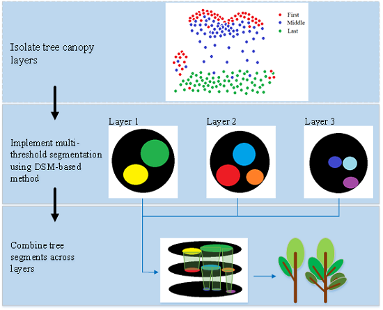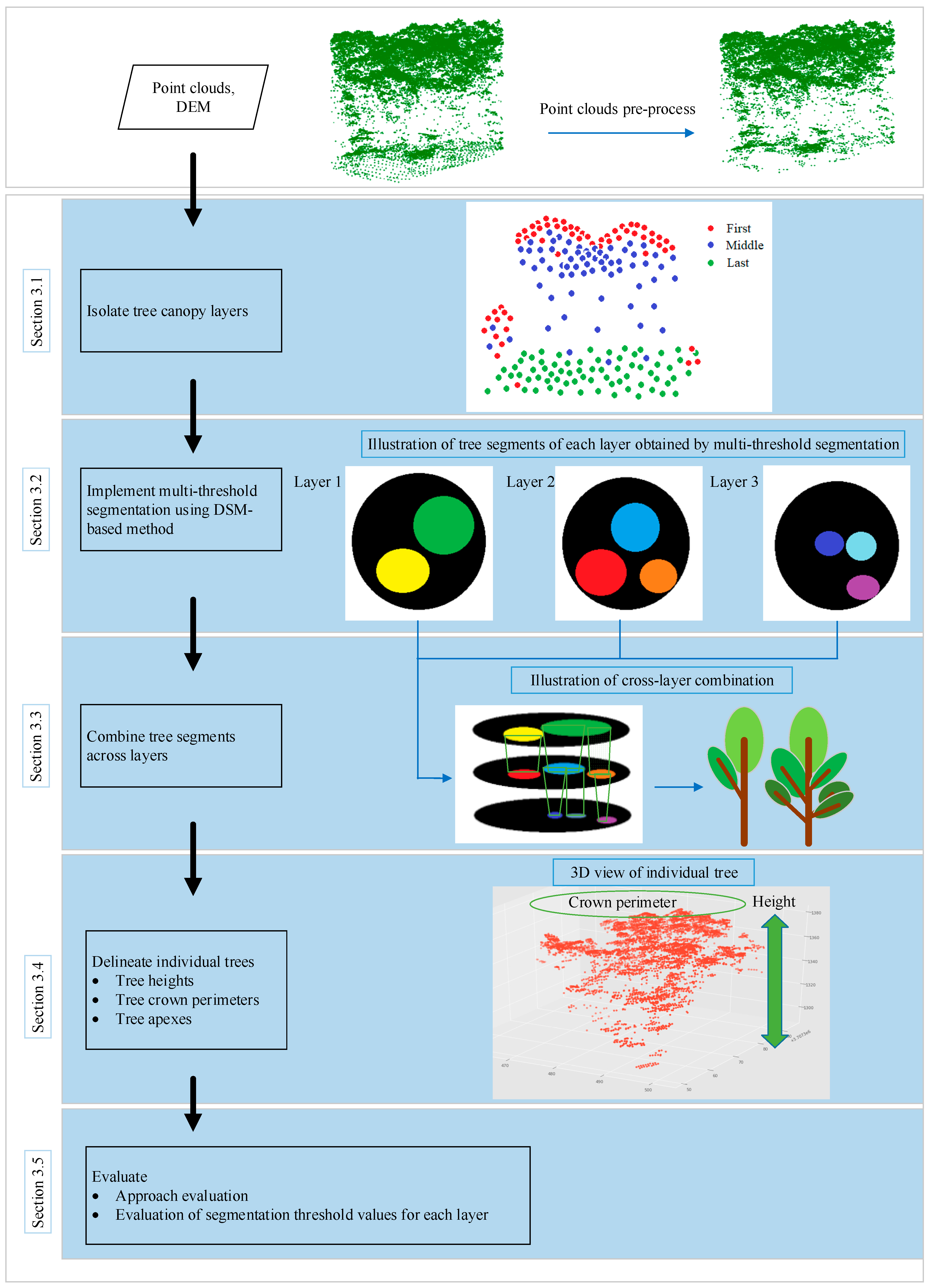Figure 1 shows the processing framework applied by our method.

3.1. Isolating Layers

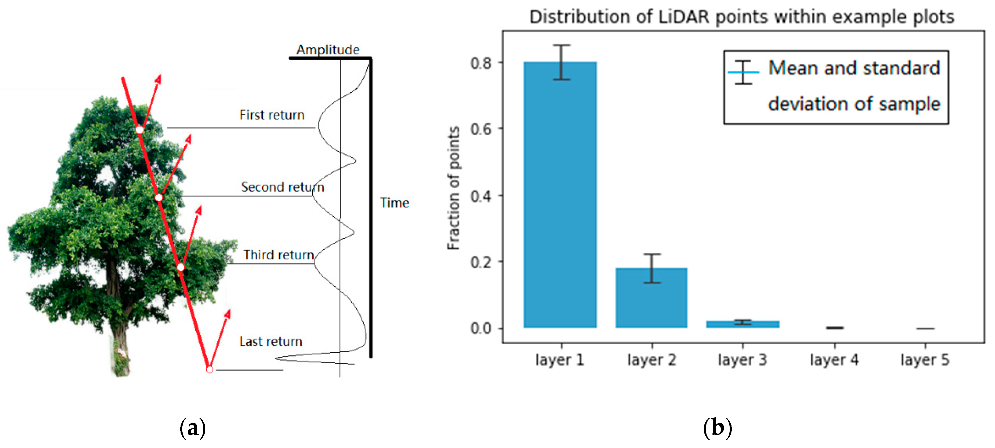
The diameter of the laser pulse is limited (~10 cm and larger). For small-footprint laser pulses, it is possible that only part of the diameter across an object. This part of the pulse reflects from there, and the rest of the pulse keeps travelling until it meets other objects which result in reflection of other parts of the pulse. After receiving the reflected laser pulse, the detector is triggered when the in-coming pulse reaches the set threshold so as to measure the flight time. The received laser pulse samples all return which are above the threshold at different stages of the reflected laser waveform. Accordingly, the range is measured to each of those points wherefrom a return occurred to yield their coordinates (Figure 2a).

Therefore, to a certain extent, the distribution of lidar return points reflects the degree of leaf overlap. Within overstory and understory, there are more return points where the leaves are denser and vice versa, which characterizes the vertical structure of the vegetation. As shown in Figure 3, point clouds of different layers can depict the tree canopies at different height levels.

Because of the penetration and multi-return characteristics of LiDAR, it offers an opportunity to capture the vegetation structure [39]; we vertically stratified each point cloud into several canopy layers by the LiDAR return number for the 271 plots and coded them into the first to fifth (Figure 2b). The layers with total heights below the minimum height of 5 m were eliminated due to being related to ground-level vegetation. Stratification did not identify any layers for plots without enough large trees and up to five layers for plots with very complex crown structures. We counted the number of points within each layer of the 271 plots and found that the amount of LiDAR points decreased as the number of LiDAR returns increased. The amount of LiDAR points within the first layer was the largest, and the percentage of numbers in the third layer was less than 5% (Figure 2b). The point density below the third layer is too low, resulting in insufficient points to characterize the vegetation. Therefore, LiDAR return points within layers 4 and 5 were combined into layer 3 point clouds in this project. The stratification strategy based on the lidar return number facilitates segmenting the lower tree canopies using the DSM-based method, which focuses on the surface points during tree segmentation.

3.2. Implementing the Multi-Threshold Segmentation Using DSM-Based Method

3.2.1. DSM-Based Method

According to the DSM-based segmentation proposed by Hamraz et al. (2016) [26], after the pre-processing steps, the tree segmentation is implemented according to the following routines: (1) locate the global maximum elevation (GMX) amongst LSPs, which is assumed to represent the apex of the highest tree within a given region; (2) generate vertical profiles originating from the GMX location and extending outwards; (3) identify the individual LSP along the profile that may represent the tree canopy boundary using adjacent trees gap recognition and local minima (LM) recognition for each profile; (4) create a convex hull along boundary points to delineate the tree canopy; and (5) cluster all LSPs encompassed within the convex hull and assign them as the current highest tree canopy. These routines are applied iteratively until all LSPs have been clustered into tree canopies. Figure 4 is an illustration of the five routines within the DSM-based tree segmentation approach.

During profile generating, the number of profiles required to smoothly represent tree canopies is determined dynamically according to LiDAR-detected canopy radii. The procedure starts with eight uniformly spaced profiles in angular (every 45°). After the tree canopy boundary and thus radius is determined for each profile (described below), the maximum tree canopy radius (r) is used to determine the chord height (x) between two maximum tree canopy radius profiles separated by the angular spacing (φ) (Figure 5) as follows:

$$x=r(1-\cos (\raisebox{1ex}{$\varphi $}\!\left/ \!\raisebox{-1ex}{$2$}\right.)),$$

(1)

If the chord height is larger than NPS, the angular spacing is reduced by half and the number of profiles is doubled.

3.2.2. Multiple Resolution Threshold Segmentation for Stratified Canopy Layers

For the DSM-based segmentation approach, grids with resolution equal to the average NPS are created by homogenizing the point spacing; LSPs are then obtained to perform segmentation. However, grids with the fixed resolution are not appropriate for multi-layer segmentation because the point spacing (or point density) is inconsistent for over- and understory trees. Therefore, it is assumed that better performance can be achieved by implementing multi-resolution threshold segmentation. To obtain different segmentation resolution, during the procedure of profile generation, we set the resolution threshold (TH) of each layer to be variable rather than rigidly equal to NPS; their values are calculated as follows:

$$T{H}_i=A_i\times NPS,$$

(2)

where i denotes the number of layers, TH_i denotes the threshold value of layer i is A times of NPS. The flowchart of the improved DSM-based segmentation method is shown in Figure 6.

During multiple resolution threshold segmentation of the isolated canopy layers, different from the direct segmentation of the first layer, the lidar point return number of the second and third layers should be set to the first return number as LSPs to implement DSM-based segmentation. The segmentation threshold of each layer is set to different values, and the optimal value of each layer is analyzed in detail in Section 3.5.2. A detailed description of the routines is given in the following: (1) isolate canopy layers for a given plot according to lidar point return number; (2) set the lidar point return number of the second and third layers to first return number, respectively; (3) assign the optimal resolution threshold value TH_i to layer i as its segmentation threshold; and (4) implement the improved DSM-based segmentation for each canopy layer. An example of multiple resolution threshold segmentation for isolated canopy layers using improved DSM-based method is shown in Figure 7.

3.3. Combining Tree Segments across Layers

3.3.1. Combination Results with the Resolution Threshold Value

After implementing multiple resolution threshold segmentation for each layer, all segments within adjacent layers are traversed systematically to determine whether they meet the merging criteria, and the regions that meet the criteria are connected. The remaining connected regions constitute the final segmentation result. The combination of segments in vertical neighboring layers contains the following cases, as shown in Figure 8a:

• New connected regions appear, such as R₁, R₂, R₃, and R₄;
• The area of the connected regions increases (or remains unchanged), such as R₅ and R₆;
• Two or more small connected regions merge into a larger one, such as R₇ and R₈.

The number of vertical neighboring connected regions contained in the large area connected region R_i can be divided into the following:

• 0, indicating that R_i is a newly generated connected region, such as R₁;
• 1, indicating that the connected region already exists, and only an increase of area is possible, such R₆;
• 2, indicating that two small connected regions grow and merge into R_i, such as R₈;
• >2, indicating that several small connected regions grow and merge into R_i, but the merging sequence is ambiguous, which is not conducive to analysis. In general, it is prevented by adding a threshold.

According to the above analysis method, the tree structure shown in Figure 8b can be established, which is called “connected growth tree” (CGT). It demonstrates the combination of nodes within different layers, in which each node denotes a connected region under the threshold value. The key of the algorithm is to determine the reasonable merging criteria.

3.3.2. Criteria for Connected Regions Merging

We assume that the connected regions of the LiDAR point cloud at coordinates (x, y, z) are E(x, y, z) when the segmentation threshold is TH_i. To introduce the merging criteria, we first define the following new measurements:

1. Connectome element

The point cloud subset of the maximum connected region that does not merge at the same horizontal position (x, y) is defined as the connectome element: E_V = E(x, y; TH₁), …, E(x, y; TH_K), where, TH₁ > … > TH_K, K is the segmentation threshold series. The connectome elements meet the following conditions:

(1)

If the connected region E(x′, y′; TH_i) is independent of E(x, y; TH_i), namely E(x, y; TH_i) ∩ E(x′, y′; TH_i) = ø, then E(x′, y′; TH_i) ∩ E(x, y; TH_i+1) = ø, i =1, 2, … K-1;

(2)

If any E(x, y; TH′) ∉ E_V (TH′ > TH₁ or TH′ < TH_K) is added into E_V, then E_V no longer meets the condition 1), then

The E_V describes the growth process of the independent child node, forms an irregular trapezoid body, and is termed a connectome element such as R₂ and R₆ as shown in Figure 8a.

2. Rate of connectome element intersection area

$$\mathsf{\Delta }{\mathrm{S}}_1=\frac{S_{\mathrm{inter}}}{S(x,y,T{H}_i)},$$

(3)

$$\mathsf{\Delta }{\mathrm{S}}_2=\frac{S_{\mathrm{inter}}}{S(x,y,T{H}_{i+1})},$$

(4)

where, S(x, y; TH_i+1) and S(x, y; TH_i) are the areas of the root node and child node, respectively; S_inter is their intersection area. Both ΔS₁ and ΔS₂ are the rates of connectome element intersection area.

Based on the above, the merging criteria of the connectome elements is:

If [(ΔS₁ > ε) ∪ (ΔS₂ > ε)] = 1, then connectome elements are allowed to merge; otherwise, they are considered independent and prohibited from merging. Where ε is a constant criterion in the range interval, 0.5, 1.0, for which 0.8 is an ideal value in our study case.

Individual tree canopies are extracted during the forest traversal process by merging the vertical neighboring tree segments from layers at a different height level (Figure 9).

3.4. Delineating Individual Trees

After the cross-layer combination of tree segments, each individual tree was delineated, their point clouds, as well as boundary points, were determined. Tree structure attributes, such as tree apex location, tree height, crown perimeter, and the number density of tree, can be obtained directly from the combined points. From these attributes, other forest parameters, such as Diameter at Breast Height (DBH), Crown Base Height (CBH), Basal Area (BA), Leaf Area Index (LAI), biomass and tree species, could be estimated using allometric equations. In this paper, our main objective was to highlight a method to accurately detect and delineate single trees from LiDAR data; we focused on two parameters which had been on-site measured values from a field survey, namely, tree location and height.

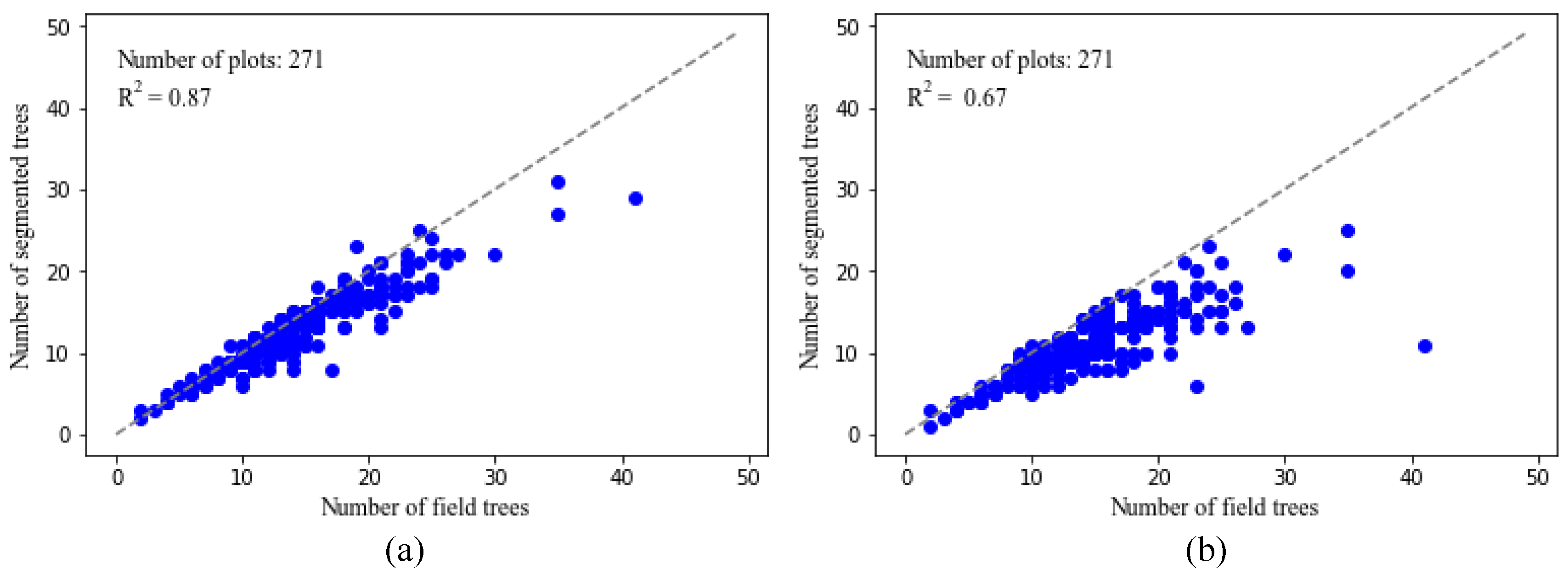
The highest point among the point cloud of each segmented tree is considered as the tree apex, and the distance from the tree apex to the ground is regarded as the height of that tree. Since the performance of trunk detection depends on the lidar point density and the forest structure, not all tree trunks can be correctly extracted [27]; the apex of the LiDAR-derived tree is considered as its location in this paper. Figure 10a,b show the comparison between the original and segmented point clouds for one of the 271 plots. It is apparent visually that most of the trees are correctly delineated. The tree delineated results in other plots in our study are similar and hence are not shown here.

3.5. Evaluating

3.5.1. Approach Evaluation

To verify the accuracy of multi-threshold segmentation, local maximum algorithms were used to identify treetops and then the semi-automatic method proposed by Kaiguang Zhao et al. (2018) [40] to match the LiDAR-derived and the field trees. Given two datasets, such as A and B, any point in dataset A can find a closest point in dataset B and vice versa. However, the identified point in dataset B has a closest point in dataset A that is not necessarily the original A point. This approach is a variant of the concept of Hausdorff distance and can be employed to help to pair trees. In this study, we paired a tree location in one dataset to another in a second dataset only if the two tree locations were the closest points to each other—a rule originally proposed by Yu et al. (2006) [41]. The distance between two locations—(x₁, y₁, z₁) and (x₂, y₂, z₂)—was calculated using the particular distance metric:

$$\mathrm{D}=\sqrt{\underset{planimetric distance}{\underbrace{{\left(x_1-x_2\right)}^2+{\left(y_1-y_2\right)}^2}}+w·\underset{height diff}{\underbrace{{\left(z_1-z_2\right)}^2}}},$$

(5)

where, (x₁, y₁, z₁) denotes apex location of the LiDAR-derived tree, (x₂, y₂) and z₂ denote stem location and tree height measured in the field, respectively. The user-defined parameter w weights the vertical distance difference against the planimetric distance; here, a value of 0.5 was used for w as a simple, empirical choice. Using the distance metric of Equation (5), the above matching approach was run to automatically obtain a preliminary list of paired trees. As a further step, it then selects the set of pairs with the smallest distance where LiDAR-derived or field tree location appears not more than once using the Hungarian allocation algorithm and regards the dataset as the matched trees [26].

The number of matched trees (MT) characterizes the segmentation quality; the number of omission errors (OE) and commission errors (CE) represents the under- and over-segmentation, respectively. The accuracy of the method was evaluated in terms of recall (Re), precision (Pr) and F-score (F) using the following equations [42]:

$$\mathrm{Re}=\frac{MT}{MT+OE},$$

(6)

$$\mathrm{Pr}=\frac{MT}{MT+CE},$$

(7)

$$\mathrm{F}=2\times \frac{\mathrm{Re}\times \mathrm{Pr}}{\mathrm{Re}+\mathrm{Pr}},$$

(8)

Re is a measure of tree detection rate, Pr is a measure of correctness of detected trees, and F is a measure of overall accuracy, taking CE and OE into account.

3.5.2. Evaluation of Segmentation Threshold Values for Each Layer

Among the 271 plots of Robinson Forest, 90 plots (about one-third of the 271 the plots) were randomly selected as a dataset to test resolution threshold effect on segmentation of different canopy layers, and the experiment of multi-threshold tree segmentation was then carried out in the remaining 181 plots using the obtained optimal thresholds. In this paper, the effect of different resolution thresholds on the segmentation accuracy of each layer is cross-tested. Using Equation (2) (see Section 3.2.2), the segmentation threshold of one of the three layers was tested, while that of the other two layers were fixed, i.e., TH_i equals to NPS (0.258 m). The experimental results are shown in Figure 11.

Figure 11 shows the tree segmentation accuracy scores using multiple resolution thresholds within the 90 plots. As shown, for over- and under-story trees, when the resolution thresholds of the three layers are increased, Pr tends to decrease slightly, which is compensated by increases in Re, resulting in a stable F-score. For the resolution thresholds TH1, TH2, and TH3 of the first, second and third layers, the metrics tend to be stable when they exceed 1.2*NPS, 1.5*NPS, and 2*NPS, respectively. Therefore, in this paper, we set thresholds of segmentation resolution of three layers equal to 1.2*NPS, 1.5*NPS, and 2*NPS, respectively. For understory trees, the average segmentation accuracy score increases with the increase of TH2 and TH3. As shown in Figure 11, when the TH3 reaches 2* NPS, the average F-score exceeds 70%, increasing by nearly 10 percentage points. This observation indicates an increased sensitivity of multi-threshold approach to segment understory trees while barely affecting the segmentation of overstory trees, which is also an indication of sound operation of the multi-threshold procedure.

4. Results

4.1. Tree Detection Rate and Accuracy

The relationship between the number of field trees and the number of segmented trees in the 271 plots is shown in Figure 12. The correlation of multi-threshold tree segmentation is relatively strong, with the coefficient of determination R² = 0.87. In general, the number of trees is under-estimated in a deciduous forest. Compared with the DSM-based segmentation method, there are more trees detected, with an increase of R² by 20 percentage points. There are 3896 trees in total in the 271 plots; only 3535 trees were segmented using the multi-threshold tree segmentation algorithm. The algorithm correctly detected 3097 trees, falsely detected 438 trees, and missed 799 trees, with under-segmentation outweighing over-segmentation. However, utilizing the DSM-based tree segmentation algorithm, only 2967 tree were segmented; the algorithm correctly detected 2591 trees, falsely detected 376 trees, and missed 1305 trees.

The statistical results of the segmentation scores of the 271 plots are shown in Figure 13, compared with the metrics of the DSM-based tree segmentation approach, for overstory trees, Re increased by 2.6 percentage points from 92.0% to 94.6%, Pr by 1.4 percentage points from 87.1% to 88.5, and F by 2.4 percentage points from 88.5% to 90.9%. For understory trees, Re increased by 21.1 percentage points from 52.3% to 73.4%, Pr decreased by 1.8 percentage points from 88.5% to 86.7%, resulting in an increase of F by 11.7 percentage points from 65.2% to 76.9%. For all trees, Pr increased slightly by 0.3 percentage points from 87.3% to 87.6%, Re and F increased by 13 and 7.5 percentage points, from 66.5% to 79.5%, 75.1% to 82.6%, respectively.

4.2. Tree-Level Parameter Estimation

Having matched the LiDAR-derived tree with the field tree, we could carry out a performance evaluation of the tree-level parameter estimation. Two tree parameters (tree location and height) derived from the LiDAR data were validated with on-site measured tree location and height. Only correctly-detected trees were used; that is, falsely-detected trees and missed trees were not counted. Among the ground truth data, only 84 of the 271 plots (i.e., 1240 trees) have on-site measured tree height data. Using our proposed multi-threshold method and DSM-based method, there were 1135 and 897 trees correctly detected within the 84 plots, respectively. The scatterplots of LiDAR-derived vs. on-site measured tree heights for all correctly-detected trees of the two methods are shown in Figure 14a,b, respectively. A simple linear regression was used to fit the lines (marked in light blue) to each dataset. For the multi-threshold method, the value of R² was 0.95. However, for the DSM-based method, the correlation result was relatively weak with R² = 0.90.

In this study, the apex of the LiDAR-derived tree was considered as the location of the tree. Figure 15a shows the histogram of tree positioning errors (namely, the distances between the LiDAR-derived and the on-site measured values of the matched trees’ horizontal coordinates) using our proposed multi-threshold method. As a contrast, the histogram generated by the DSM-based method is given in Figure 15b. The mean differences of our proposed multi-threshold method and the DSM-based method were 82 cm and 105 cm, respectively.

After matching the lidar-derived trees with the field trees, we can also estimate the crown sizes. As shown in Figure 16, crown perimeters and heights of all of the correctly-detected trees reveal that most of the trees have a crown perimeter range of 10–40 m, and a height range of 10–30 m. Tree height and crown size distribution statistics have practical guiding significance for forest management, such as improvement cutting, forest inventory, growth forecasting, and afforestation design.

5. Discussion

In recent decades, airborne LiDAR-based remote sensing has shown promise in forest science, for characterizing the structure of forests at landscape-level, stand-level, and plot-level [9,11,23,40]. These efforts in forest quantification are currently driving improvements in forest assessment, monitoring, and management activities [2,3,40]. The correct detection and characterization of individual trees is one of the key issues in forest science, linking with biometer ecological models [43] and more precise estimations of biomass in forests [17].

However, the overall detection accuracy of trees, especially of understory trees, is relatively low in complex and closed-canopy deciduous forests [31,35]. In some studies, only about 50% [3,15] and 65% [14] of the trees are detected. Hu et al. (2014) [44] proposed an automated method using prior knowledge of tree crowns, which correctly delineated about 74% and 72% of the crowns in two stands of mixed wood and deciduous species, respectively. Duncanson et al. (2014) [9] proposed a multilayer canopy delineation method which correctly isolated 70% dominant, 58% co-dominant, 35% intermediate, and 21% suppressed trees in a closed-canopy deciduous forest. Some recent researches improved the tree detection accuracy, for example, Wanqian Yan et al. (2018) [43] developed an automated hierarchical single-tree segmentation approach, and achieved the average correctness, completeness, and overall accuracy of 90%, 88%, and 89%, respectively. Ayrey et al. (2017) [32] used a layer stacking approach which detected 79% of trees in sparse and 72% of trees in dense even-aged deciduous stands. However, the trees in these study areas were planted almost at the same time, leading to their similarities in shape and size, and segmenting trees is relatively simpler. Paris et al. (2016) [33] correctly detected 97% and 92% of the dominant trees and 77% of the sub-dominant trees with a commission rate of 7% in conifer sites. It is worth noting that, due to well-defined crown shapes, segmenting trees in coniferous forests is relatively simpler. Studies show better tree segmentation performance of coniferous forest compared to deciduous forest or mixed forest [44]. Our algorithm was tested in the University of Kentucky’s Robinson Forest—a natural deciduous forest with complex terrain and vegetation structure and as a result provided a reasonable test of universality and applicability. Overall, 79.5% of the trees in our study area were detected by the algorithm, and 87.6% of them were correctly detected; the overall accuracy, taking CE and OE into account, was 82.6%, in which 73.4% of understory trees were detected and 86.7% of them were correctly detected. Our new algorithm shows good potential to identify single trees in natural deciduous.

In a few scenarios, due to the surrounding tall trees and the airborne lidar scanning field of view (40° in our study area), some lower-altitude upper trees may not be able to be scanned directly and captured as the first return number point clouds (Figure 7a,b). 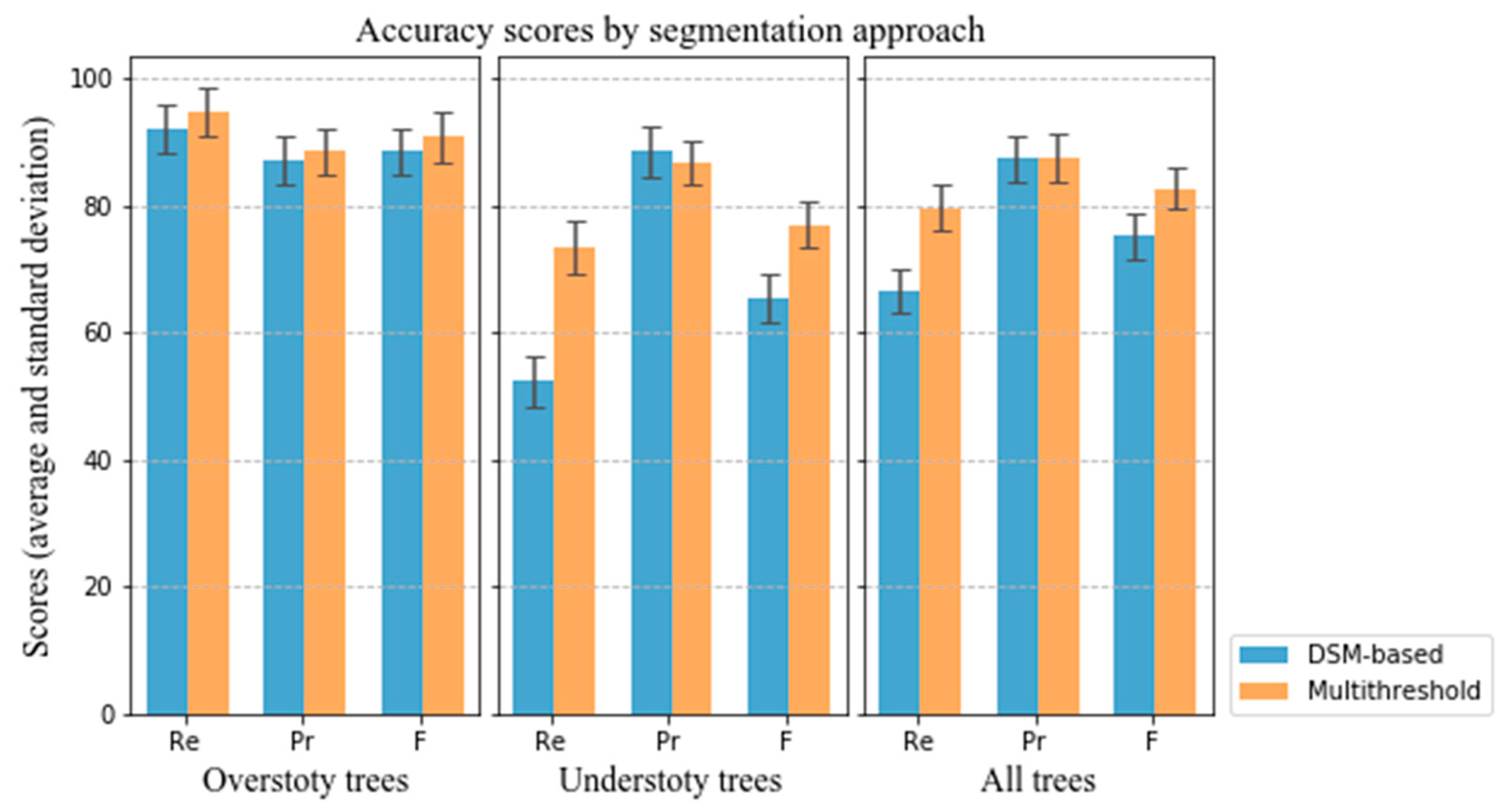In our algorithm, the hierarchical segmentation strategy based on lidar return number can effectively detect these trees to minimize under-segmenting tree crowns (Figure 7c,d). Meanwhile, our algorithm, because it makes full use of the vertical information of vegetation by canopy stratification and setting the different segmentation threshold for each canopy layer, increases the detection ration of understory trees. For further details, by comparing the segmentation scores between overstory trees and understory trees shown in Figure 13, it may be concluded that:

For the detection rate Re, the improvement in the latter is greater, which indicates that the multi-threshold segmentation can effectively detect understory vegetation;

For the correctness of detected trees Pr, the detection accuracy of understory trees decreases with the increase of detection rate. The main reasons are as follows: On the one hand, the detection rate of lower trees improved, and the number of detected trees increased. On the other hand, due to the occlusion effect of higher vegetation layer, the pulse penetration rate of lidar and point density of the lower vegetation are reduced, which limits the improvement of segmentation accuracy. These two factors lead to a decrease of detection accuracy of multi-threshold segmentation method for understory trees compared with DSM-based method;

For the overall accuracy F, the latter improves more. Although the accuracy of the detection rate decreases slightly, the detection rate is improved, which leads to the improvement of the overall segmentation accuracy. This proves the effectiveness of the multi-threshold method for the segmentation of undergrowth trees.

By comparing the overall accuracy F for all trees, the multi-threshold tree segmentation approach has a higher score. As noted, DSM-based and other CHM-based algorithms might not perform well in deciduous forests with dense interlocking crowns lacking distinct peaks and troughs. However, the proposed method implements multi-threshold segmentation for different canopy layers and combines tree segments of each layer according to the characteristics of vegetation structure, which leads to improve the detection rate of lower vegetation and reduce over- and under-segmentation (Figure 7 and Figure 10).

Due to the importance of the ecological environment and the increasing demand for precise forestry, more and more forestry researches focus on the identification and parameter estimation of individual trees at tree-level. Some recent studies have focused on the use of understory vegetation information to improve detection accuracy. For example, Wei et al. (2018) [27] used the trunk detection-aided mean shift clustering techniques to delineate individual and estimate tree structural parameters. Hamraz et al. (2017) [35] proposed a stratification-enabled tree segmentation approach, which stripped the canopies one by one to detect understory trees. The similarity between these methods and the method proposed in this paper lies in that they all aim to improve the detection rate of understory trees through the information of low canopies. The difference or novelty of our method lies in that, first, so far, little literature has studied the effect of threshold sizes on the segmentation of canopy layers’ point clouds with different point density. For the stratification-enabled tree segmentation approach proposed by Hamraz et al. (2017) [35], DSM-based tree segmentation is implemented on the stripped canopy layers to detect understory trees. However, this method implements a segmenting routine with a fixed threshold for overstory and understory, ignoring the difference of their lidar point densities between overstory and understory, which leads to over-segmentation of the understory trees. In our approach, we tried to implement multi-resolution threshold segmentation for canopy layers to obtain better performance. Second, Hamraz et al. (2017) [35] stripped the canopy according to the height histogram of lidar points. In contrast, for the first time, we stratified the canopy according to the lidar return number. This technique can dynamically acquire the vertical structure characteristics of vegetation without statistic the distribution of lidar points and a priori assumptions about tree canopy shape or size. Finally, in our algorithm, a cross-layer combination rule was proposed to merge the tree segments belonging to the same tree, which makes full use of the spatial relationship of tree canopies and reduces over-segmentation.

In our algorithm, the major limitation or the biggest uncertainty in tree segmentation mainly derives from two aspects: On the one hand, according to the cross-layer combination rule, when the overlap area of adjacent canopy segments is more than a certain value (equal to 0.8), they will be considered as a crown of the same tree to be combined. Therefore, when a small tree is completely within the vertical projection of the crown of a large tree, the small one may be considered as a part of the big one and not be detected by our algorithm. However, in the natural environment, tree growth is often limited to light availability. Trees that are completely under the crown of a large tree receive very little light and may not grow very high. Therefore, they will be considered as low-vegetation and eliminated. On the other hand, it is worth noting that the algorithm is sensitive to the segmentation threshold of each canopy layer. In this paper, the segmentation effect of each canopy layer on the sample plots is cross-tested, and the optimal segmentation threshold of each layer is then obtained by statistical analysis. Since the plots of the study area in this paper belong to the same natural deciduous forest with similar terrain and vegetation conditions, the segmentation threshold of each canopy layer is sufficient in this study. In other forests, the segmentation threshold of each canopy layer should be redetermined according to their terrain, vegetation conditions, and lidar point density. To obtain the adaptive tree segmentation thresholds of different forests, we plan to obtain segmentation thresholds by using deep learning algorithm in future work.

6. Conclusions

This paper proposed a multi-threshold single-tree segmentation approach using small-footprint airborne LiDAR data, which consists of data pre-processing and isolating canopy layers, multiple resolution threshold segmentation for isolated layers, cross-layer combination of tree segments, delineation of individual trees, and tree parameter extraction. It is an improved hierarchical scheme incorporating a multiple threshold segmentation strategy, which has the promise to be successfully applied to natural deciduous forests. By applying the proposed approach to airborne LiDAR data acquired in a closed-canopy deciduous forest located in southeastern Kentucky and comparing it with existing point-based methods in terms of overall tree detection rates and tree-level parameter estimation accuracy, we have shown that the multi-threshold segmentation can lead to significant performance improvements in single tree-level forest inventory. Our approach is robust and effective for delineating individual trees from airborne LiDAR data since: (1) multi-threshold method facilitates to improve the detection rate of understory with low point density; (2) the cross-layer combination of tree segments makes full use of vertical information of the tree, reduces over-segmentation, and improves accuracy of tree detection; and (3) the encoded canopy layers for segmenting are determined according to the lidar return number without a priori assumptions about tree canopy shape or size, leading to capture the local information of the canopy dynamically and to use it to improve delineating the contour of the crown.