Global Detection of Long-Term (1982–2017) Burned Area with AVHRR-LTDR Data

Abstract

This paper presents the first global burned area (BA) product derived from the land long term data record (LTDR), a long-term 0.05-degree resolution dataset generated from advanced very high resolution radiometer (AVHRR) images. Daily images were combined in monthly composites using the maximum temperature criterion to enhance the burned signal and eliminate clouds and artifacts. A synthetic BA index was created to improve the detection of the BA signal. This index included red and near infrared reflectance, surface temperature, two spectral indices, and their temporal differences. Monthly models were generated using the random forest classifier, using the twelve monthly composites of each year as the predictors. Training data were obtained from the NASA MCD64A1 collection 6 product (500 m spatial resolution) for eight years of the overlapping period (2001–2017). This included some years with low and high fire occurrence. Results were tested with the remaining eight years. Pixels classified as burned were converted to burned proportions using the MCD64A1 product. The final product (named FireCCILT10) estimated BA in 0.05-degree cells for the 1982 to 2017 period (excluding 1994, due to input data gaps). This product is the longest global BA currently available, extending almost 20 years back from the existing NASA and ESA BA products. BA estimations from the FireCCILT10 product were compared with those from the MCD64A1 product for continental regions, obtaining high correlation values (r² 0.9), with better agreement in tropical regions rather than boreal regions. The annual average of BA of the time series was 3.12 Mkm². Tropical Africa had the highest proportion of burnings, accounting for 74.37% of global BA. Spatial trends were found to be similar to existing global BA products, but temporal trends showed unstable annual variations, most likely linked to the changes in the AVHRR sensor and orbital decays of the NOAA satellites.

1. Introduction

The Global Climate Observing System (GCOS) program and the Intergovernmental Panel on Climate Change (IPCC) assessment report [1] consider fire occurrence as one of the essential climate variables (ECV) because of its great impact on atmospheric emissions and vegetation dynamics [2,3,4,5,6]. Climate modelers need information about the burned area (BA) to improve their knowledge on its role on climate dynamics. For this reason, most of the existing climate models include a fire module [7].

Historical data on fires have been obtained through national fire statistics or from field studies [8,9]. These data have been used to generate global estimates of fire occurrence using different interpolation techniques [8]. In the early 2000s, the first estimations of global BA derived from satellite earth observation were produced [10]. Those products were derived from the SPOT-VEGETATION sensor at a 1 km resolution, first for the year 2000 [11] and then extended using similar BA algorithms for the period 2000–2007 [12]. More recently, similar approaches have been used to generate BA products from the Proba-V sensor, with 333 m resolution [13]. NASA began generating BA products from images acquired by the MODIS sensor in the early 2000s. Two products were released from this sensor, MCD45A1 [14] and MCD64A1 [15], both at a 500 m spatial resolution. The latter product was also the basis of the Global Fire Emission Database (GFED, now at v4, [16]). From the highest resolution bands of MODIS (at 250 m), a recent BA product has been released from the European Space Agency’s Fire_cci project [17].

All of these global products have a relatively short time series (2001 to the present), with the exception of the GFED, which extends to 1995, but contains higher uncertainties for the pre-MODIS era (2000). This short period limits the relevance of these datasets for analyzing the relationships between climate and fire activity. For this reason, the use of advanced very high resolution radiometer (AVHRR) images is very appealing, as this sensor provides much longer temporal coverage than MODIS or SPOT-VEGETATION, spanning from 1979 to the present. Unfortunately, the AVHRR sensor has lower radiometric and geometric quality, with a 1.1 km spatial resolution at the nadir. In addition, the global archive of the full resolution AVHRR data only began in the early 1990s, so images acquired in the 1980s are only available at a degraded resolution (4 km or lower). Therefore, deriving global and accurate BA information from these data is very challenging. The AVHRR time series has been used in different regional studies to derive the BA time series, either at the full resolution of this sensor for particular regions [18,19,20] or using coarser resolution versions (8 km) with examples in Africa [21], Canada [22], Russia [23], and global coverage for the 1981–2000 period [24]. These studies have provided moderately accurate values when compared to other BA products due to the spatial and radiometric limitations of AVHRR sensors.

Despite these limitations, obtaining long BA time series from AVHRR images would be very beneficial for climate modelers as it would provide a significant temporal extension to the current BA products. This was the main motivation to conduct the present research, which was developed within the ESA Climate Change Initiative (CCI) program’s Fire_cci project [25]. Considering the existing AVHRR time series products, we selected the land long term data record (LTDR), which covers 1981–to the present at a 0.05 degree resolution (≈5 km) including acquisitions from seven different NOAA satellites [26]. LTDR is the highest spatial resolution dataset of AVHRR images that globally covers the full lifetime of the sensor. The objective of this paper was to present the development of an algorithm to detect BA pixels from LTDR data, and analyze the outputs in relation to other existing products.

2. Methods

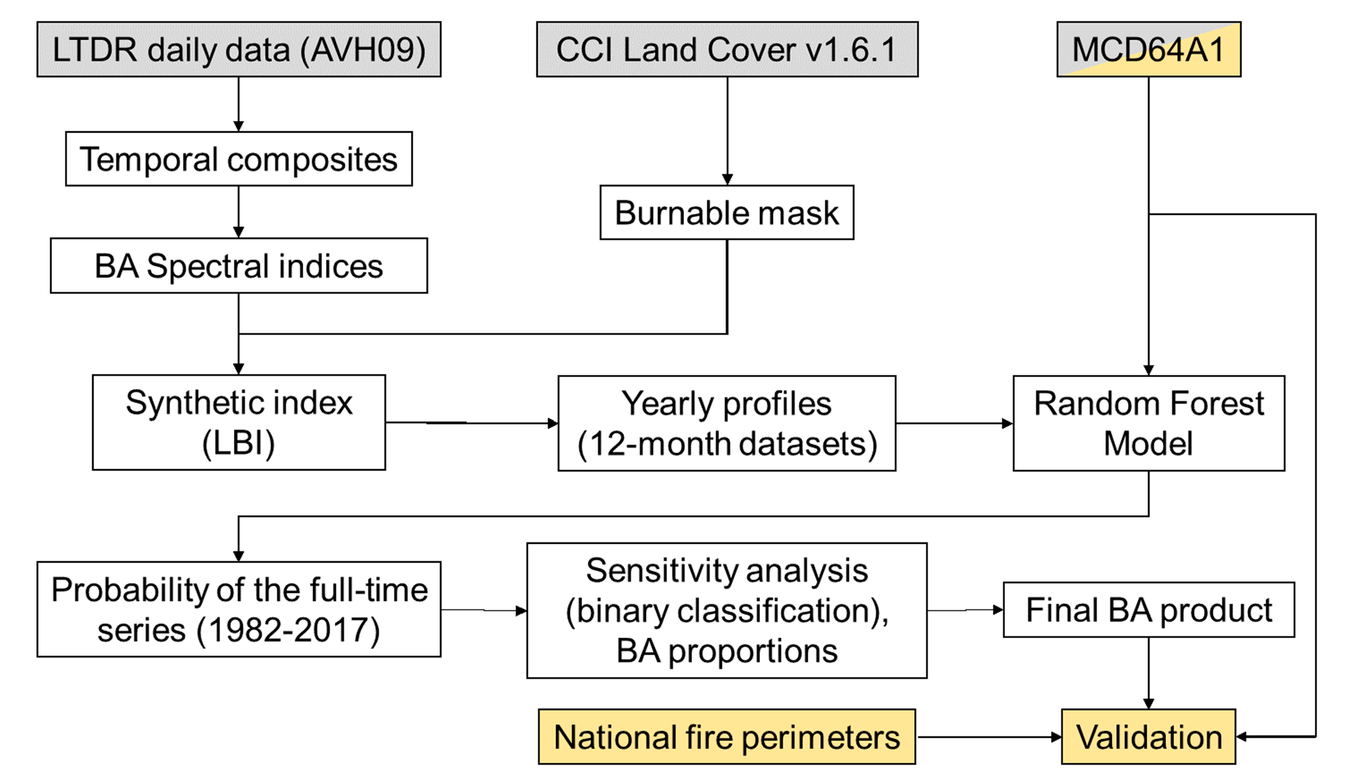
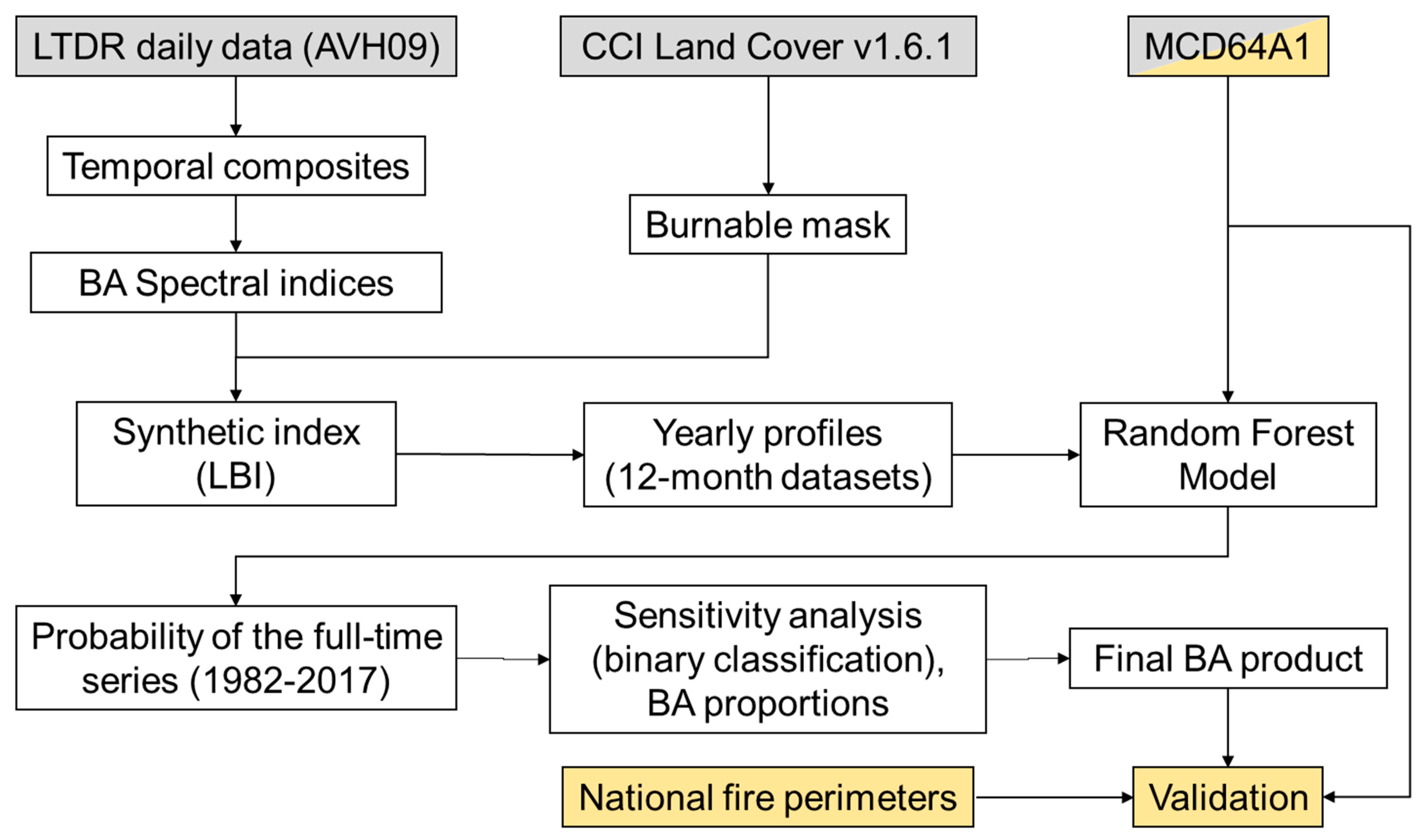
2.1. General Workflow

Figure 1 presents the flow chart with the BA algorithm structure. First, the LTDR daily data were synthetized in monthly composites and spectral indices related to the burned signal were calculated. Unburnable covers were masked out to optimize processing and avoid potential commission errors. These masked areas included bare soil, water, urban areas. and permanent snow and ice, and were obtained from the Land Cover CCI project [27]. From the input bands and derived spectral indices, a synthetic BA variable (named as the LTDR BA index, or LBI to simplify) was computed. This variable tried to include the different spectral features of AVHRR data that would help to discriminate burned pixels based on experience from previous studies and LTDR sample statistics. The random forest (RF) classifier was selected to discriminate burned and unburned pixels, as it has provided good generalization potential in many recent satellite applications. To facilitate the discrimination of BA using seasonal changes, the RF models were trained using the twelve monthly LBI values of each single year as the predictor variables. The training was based on burned pixels obtained from the NASA MCD64A1 Collection 6 (from now on simply MCD64A1) BA product [15], which produced global BA estimations from 2001 to 2017 at a 500 m spatial resolution. This product is widely used by climate modelers [28]. Previous estimations of commission and omission errors for this product were 0.336 and 0.663, respectively [29]. The MCD64A1 product was resampled at 0.05 degrees to obtain the proportion of BA within each LTDR pixel. A pixel was considered burned if it had at least 1% of BA.

The RF model was used to run the processing over the whole time series. Once the burned pixels were detected, they were assigned a proportion of BA based on the MCD64A1 dataset. Finally, the BA product (named FireCCILT10) was formatted to match the standard formats of the Fire_cci project, and made freely accessible [25]. The validation was carried out by comparing BA detections with those included in the MCD64A1 product for those years not used in the training phase. A comparison was also made with the fire perimeters derived from national services in Australia, Canada, and California. Further details are included in the following sections.

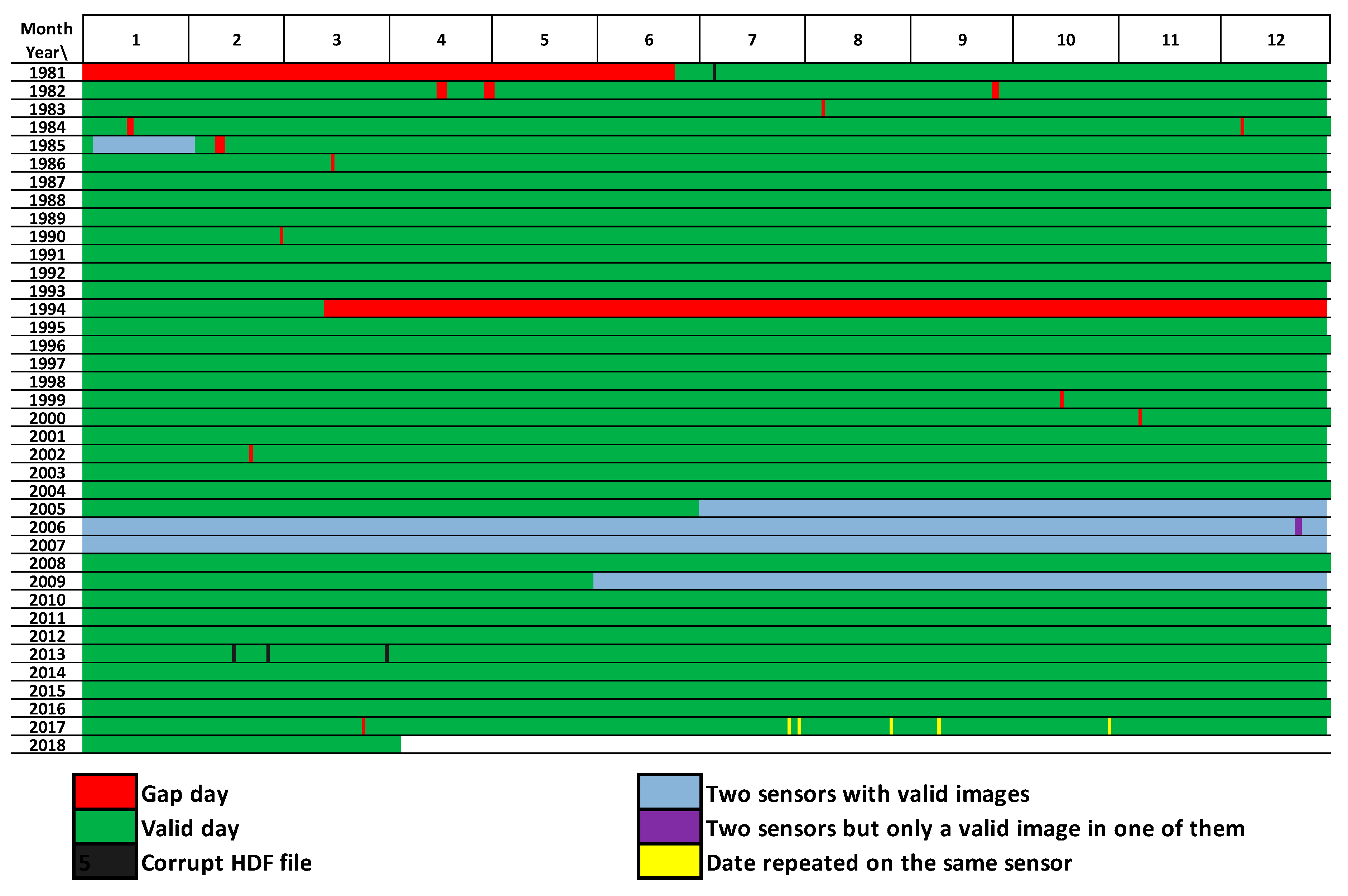
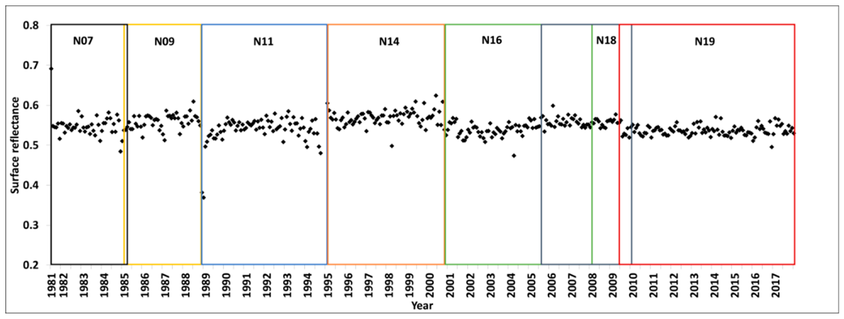
2.2. Land Long Term Data Record Dataset

The LTDR Version 5 product is a dataset created by NASA to provide a corrected time series of global AVHRR coarse-resolution observations [26]. This was generated using the global area coverage (GAC, 4 × 4 km), acquired by the AVHRR2/3 sensors on board the NOAA-7, 9, 11, 14, 16, 18, and 19 satellites (all of them have an equatorial crossing time around early afternoon). The LTDR data are available from 1981–to the present, representing the longest global time series of satellite Earth observations (38 years). However, the dataset is not fully continuous, as different observational gaps are still present. The most important one was found in 1994, which covered several months (Figure 2). For this reason, 1994 was not used in the generation of the FireCCILT10 product.

The LTDR dataset includes radiometric corrections, geometric corrections (inverse navigation to relate an Earth location to each sensor’s instantaneous field of view), and atmospheric corrections (Rayleigh scattering, ozone, water vapor, and aerosol correction). For the latter, MODIS images were used to guarantee consistency, assessing the years in which they were present within the time series. However, despite the calibration among sensors, some inconsistencies were found in the visible channels (Figure 3) due to the degradation during the sensor’s lifetime and for those periods where the new versions of the AVHRR sensor were included in the time series.

The LTDR product has ten bands. The original bands are surface reflectance for channel 1 (0.58–0.68 µm) and channel 2 (0.725–1.1 µm) (red and near infrared, respectively), medium infrared (surface reflectance and top of atmosphere (TOA) brightness temperature for channel 3, 3.55–3.93 µm), and thermal infrared (TOA brightness temperature for channel 4, 10.3–11.3 µm and TOA brightness temperature for channel 5, 11.5–12.5 µm). In addition, LTDR includes the view zenith angle, solar zenith angle, relative azimuth, and quality assessment field (QA). Two bands show several problems. First, the AVHRR2 sensor was changed for AVHRR3 in 2000 with NOAA-16. The new version of the sensor included a change of configuration in channel 3 between daytime (channel 3a, 1.58–1.64 µm) and night-time (channel 3b, the 3.55–3.93 µm original configuration), which implied a modification of daily reflectance and temperature for this band (Figure 4). In 2003, the historical configuration was restored. Furthermore, saturation of channel 3 on the AVHRR2 sensor was increased in the AVHRR3 sensor to 63 degrees [32], so this channel was also not consistent with previous versions (Figure 5). On the other hand, the QA information was found to be not sufficiently accurate as many cloudy and noise pixels observed visually were not properly masked. Therefore, this layer was finally not used.

2.3. Composites

LTDR daily data are difficult to process because they are affected by noise, clouds, shadows, very oblique angles, radiometric instability, and other artifacts. Monthly composites (Figure 6) have been commonly used instead [33] to retain the highest quality observations of a daily dataset. Among the different criteria for creating image composites, we selected the maximum temperature of channel 4 (10.3–11.3 µm), as it has been proven to provide good sensitivity to detect burned pixels while avoiding clouds and cloud shadows [34]. The compositing algorithm also included a burnable mask derived from the ESA’s CCI Land Cover v1.6.1 product [27]. The land cover product was reclassified (burnable and unburnable) and resampled from the original 300 m resolution to the LTDR resolution (0.05 degree), thus obtaining the proportion of burnable area within each pixel. All pixels with a proportion of burnable area lower than 20% were masked and discarded from the analysis. We selected the year 2000 from the different available epochs of this product as being representative of the average cover conditions of the target period.

2.4. Input Bands

To analyze the spectral separability of burned and unburned pixels, the original bands and different spectral indices previously used in BA studies and others used for vegetation dynamics were computed (

Table 1. Derived bands generated as inputs for the BA algorithm. References for previous studies using each index for BA discrimination are included.

Index	Formula	Developer	BA Application
Normalized Difference Vegetation Index	$NDVI=\frac{{\rho }_{NIR}-{\rho }_{RED}}{{\rho }_{NIR}+{\rho }_{RED}}$ ρNIR = surface reflectance for channel 2 (0.725–1.1 µm) ρRED = surface reflectance for channel 1 (0.58–0.68 µm)	[35]	[11,36]
Global Environmental Monitoring Index	$\mathrm{GEMI}=\mathsf{\eta }·\left(1-0.25·\mathsf{\eta }\right)-\left(\frac{{\rho }_{RED}-0.125}{1-{\rho }_{RED}}\right)$ $\mathsf{\eta }=\frac{\left(2 · \left({{\rho }_{NIR}}^2-{\rho }_{RED}{}^2\right)+ 1.5 ·{\rho }_{NIR}+0.5·{\rho }_{RED}\right)}{{\rho }_{NIR}+{\rho }_{RED}+0.5}$	[37]	[18,21]
Burned Area Index	$\mathrm{BAI}=\frac{1}{{\left({\rho c}_{RED}-{\rho }_{RED}\right)}^2+ {\left({\rho c}_{NIR}-{\rho }_{NIR}\right)}^2}$ Where ρcNIR and ρcRED are the convergence values for burned vegetation (defined for AVHRR as 0.06 and 0.1, respectively).	[38]	[18]
Soil Adjusted Vegetation Index	$SAVI= \frac{{\rho }_{NIR}-{\rho }_{RED}}{{\rho }_{NIR}+{\rho }_{RED}+L}·\left(1+L\right)$ Being L soil reflectance (in this case L = 0.5)	[39]	[40]
Modified Soil Adjusted Vegetation Index	$MSAVI= 0.5·[{\left(2·{\rho }_{NIR}+1\right)}^2-2\left({\left(2·{\rho }_{NIR}+1\right)}^2-8\left({\rho }_{NIR}-{\rho }_{RED}\right){)}^{\frac{1}{2}}\right]$	[41]	[21]
Surface Temperature	$Ts= \mathrm{T}4+3.33\left(\mathrm{T}4-\mathrm{T}5\right)$ T4 = TOA brightness temperature of channel 4 (~10.3–11.3 μm) T5 = TOA brightness temperature of channel 5 (~11.5–12.5 μm)	[42]	[21]

). In addition, the monthly temporal differences of those indices were also calculated.

A statistical analysis was carried out to select the most sensitive variables to discriminate between burned and unburned pixels. A sampling of more than 450,000 burned and more than 50 million unburned pixels was selected. Burned pixels were extracted from the MCD64A1 product, which was used as the reference dataset to generate the classification model. We used 2008 as the calibration year for this analysis. We computed the median and interquartile range values for each input band to analyze whether expected trends (for instance, lower NDVI for higher burned proportions) of each input band were observed. Additionally, RF models were run to select the most explicative variables for BA discrimination, but the results were not conclusive.

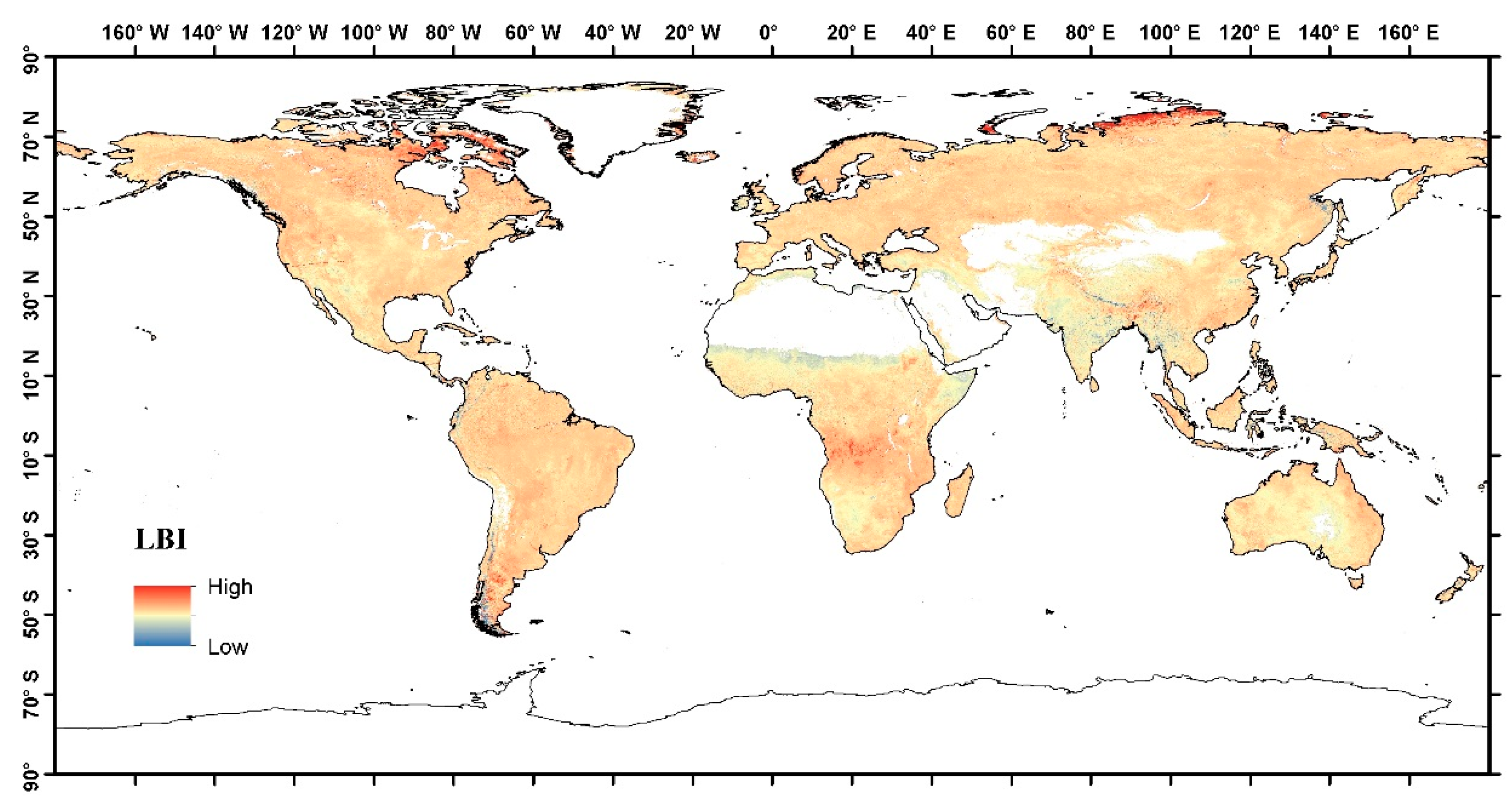
2.5. LTDR Burned Area Index

Several RF models were generated from the original and derived bands (Table 1), but the results showed severe confusion between the burned and unburned pixels. Therefore, we decided to base our models on a dedicated synthetic index that aimed to combine the most sensitive variables for BA discrimination in a single variable. We named this index, the LTDR BA Index (LBI), which included various spectral dimensions of fire effects such as low NIR and R reflectance and GEMI values, high temperature, temporal decrease in NIR reflectance and GEMI values, and increase in temperature. These trends were observed in our dataset as well as in several previous studies on BA discrimination [43].

All variables (X) were normalized (z-score), to reduce the impact of temporal instability in the time series using the means (μ) and standard deviations (σ) for each month:

$$z= \frac{X-\mathsf{\mu }}{\mathsf{\sigma }}$$

The final formula of the LBI was:

$$LBI=z\left(T5\right)-z\left(T5\_diff\right)-z\left(Red\right)-z\left(Red\_diff\right)-z\left(NIR\right)-z\left(NIR\_diff\right)-z\left(GEMI\right)-z\left(BAI\right)-z\left(BA{I}_t+1\right)$$

where t is the monthly composite being analyzed; t + 1 is the composite of the following month and t − 1 is the composite of the previous month; diff is the difference between t − 1 and t; T5 is the TOA brightness temperature of channel 5 (~11.5–12.5 μm); Red is the surface reflectance of channel 1 (0.5–0.7 μm); and NIR is the surface reflectance of channel 2 (0.7–1.0 μm).

Figure 7 shows the comparison of monthly LBI values for the burned and unburned pixels in different tropical regions [44]. To facilitate the comparison between pixels in different hemispheres, the figure indicates the months before and after the fire occurrence. The higher values of LBI indicate a higher likelihood of burning. The burned pixel shows a clear variation around the date of the burning, while the unburned shows a more stable trend. The increase of LBI values before the fire may be related to an increase in vegetation dryness (thus reducing chlorophyll activity) and temperature.

Figure 8 shows the global LBI values in July 2008. As expected, larger values were observed in the Southern Tropical fringe of Africa, which commonly burns during this period. Great values were also observed at high latitudes (60°) where the quality of the LTDR data decreased or artifacts were observed. These outliers did not affect BA discrimination as their temporal trend did not show the clear seasonal variability observed for burned pixels.

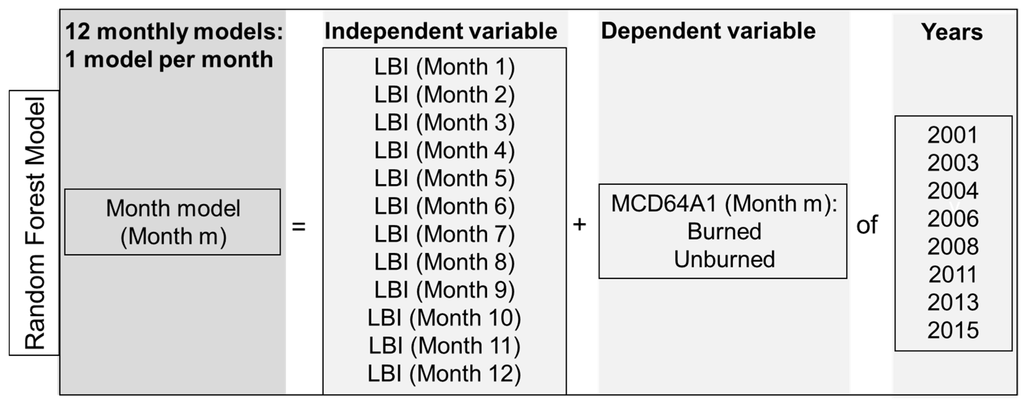
2.6. Random Forest Model

The RF algorithm was selected to create the LTDR BA classification because it has been shown to be quite robust in many land cover classification studies [45,46,47] that also includes BA discrimination [48,49,50]. RF is a machine learning algorithm that is based on generating a combination of decision trees that are independent of each other. Each decision tree randomly selects a subset of input pixels, which are discriminated using the predictor variables. A pixel is assigned to a category according to the majority vote of the ensemble of trees.

For this particular classification, the RF parameters were defined following our previous studies [48,49]. Six hundred decision trees were selected as this was found to be a good number to reach that had acceptable precision without greatly increasing the processing time. To cope with the high unbalanced character of our sample (the vast majority of pixels were unburned), a 10% proportion of the BA pixels were forced to be included in each decision tree. The data entered in each tree were selected randomly, establishing only the percentage of each class.

Monthly RF models were developed to better adjust the fire conditions of each month. Several factors were considered to build the RF models: (1) the number of months during the year by analyzing the impact of the temporal seasonality on the models; (2) the number of input years to be able to obtain a generalized model that was valid for the full time series; and (3) the proportions of the burned area in the MCD64A1 that should define a pixel as burned.

RF models were run with a different number of input months within a year. When just using three months (t, t − 1 and t + 1) the model did not show good performance. The number of months was subsequently increased from seven (three months before, month of study, and three months after) to the whole year to further consider seasonal variability. The latter showed the best performance, as the 12 months included a more complete temporal evolution of the pre- and post-fire conditions.

The first RF models were trained with only one year (2008), but the resultant model performed poorly in other years. Therefore, training was based on several sets of years to avoid the overtraining bias. We found a stable and consistent model with eight years of training data (2001, 2003, 2004, 2006, 2008, 2011, 2013, and 2015) and included years with different global fire occurrences such as 2004 and 2011, which had the highest occurrence, and 2013, which had the lowest.

Finally, different RF models were trained with several proportions of BA within a pixel by taking this information from the reference MCD64A1 product. Five percentile classes (0, 25, 25–50, 50–75, 75), four classes (0, 40, 40–80, 80), three classes (0, 50, 50), and two classes (0, 80) were tested. They showed severe overtraining or inaccurate results, since most of the burned pixels were in the low percentage range. Finally, two classes (burned/unburned) were used, where burned was classified as those LTDR pixels with any proportion of burned (=1%).

In summary, our BA product (named FireCCILT10) was based on 12 RF monthly models, each trained with eight years of data and with two output classes (burned/unburned) (Figure 9). In all cases, the predictor variables were the 12 monthly LBI values of each input year. The training dataset had around one million burned pixels and around thirty million unburned pixels. The RF classification was performed with the monthly models and for the full time series of the LTDR dataset excluding the year 1994. A total of 420 classifications (12 months × 35 years) were performed to obtain the final product. The RF output provided the probability (between 0 and 1) of a pixel to be burned per month and year.

A sensitivity analysis was carried out to convert the RF probabilities into a binary classification, using MCD64A1 data for the overlapping period (2001–2016). Different cut-off thresholds (between 0.00 and 1.00) were used to evaluate the ones that classified the LTDR pixels more similarly to the MCD64A1 product. The proportion with the highest dice coefficient (DC) for each month was used. DC is a statistical index that integrates the omission and commission error of the BA class [51]. Since each year showed slight variations in the monthly thresholds, we used the median value of all years for each month as a cut off value for that month to obtain the burned–unburned classification during the whole time series. The RF probability of the burned assignment was also kept to compute the uncertainty of the BA detection, which was offered as an auxiliary variable of the final FireCCILT10 product.

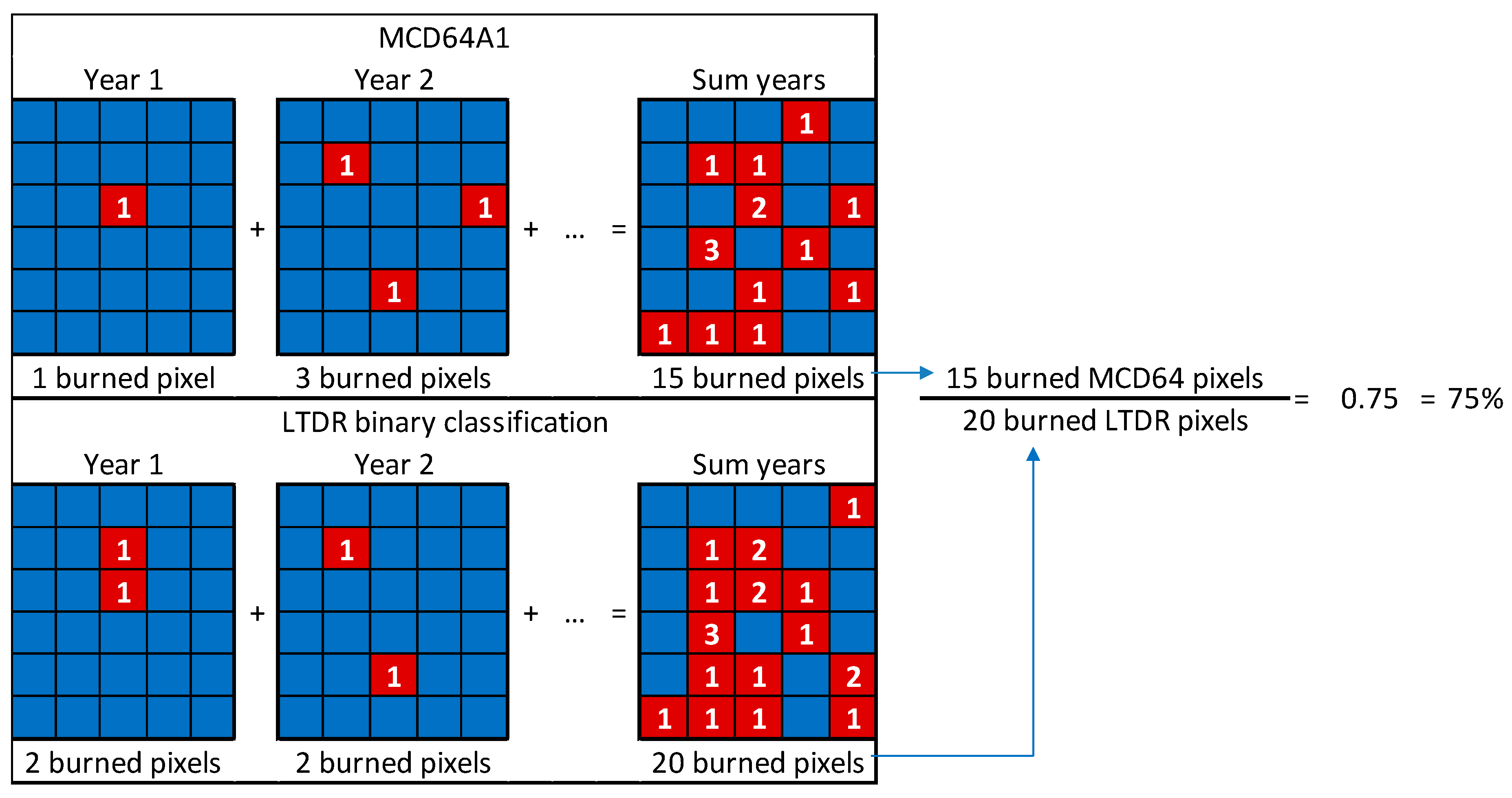
2.7. Estimation of Burned Proportions

Once the binary classification was obtained, the final phase was to assign a certain proportion of the burned area to each burned pixel. Considering a burned LTDR pixel as fully burned was not realistic, as it is unlikely that such a large area (around 25 km²) would be completely affected by fires. For this reason, the pixels classified as burned were converted to a proportion of burned using the MCD64A1 product as a proxy of the true BA. The aim was to obtain a relationship that would provide a similar total BA to the MCD64A1 and LTDR products for the overlapping period, and then use that relation to extrapolate backwards.

This analysis was performed at a grid-cell level, with cells having a 0.25-degree spatial resolution (5 × 5 LTDR pixels). First, we computed the actual BA for each cell during the overlapping period from the MCD64A1. Then, for each cell, we estimated the proportion of burned pixels that would sum up the total BA estimated by the MCD64A1 product (Figure 10). This process was done for each cell and each month of the existing MCD64A1 time series.

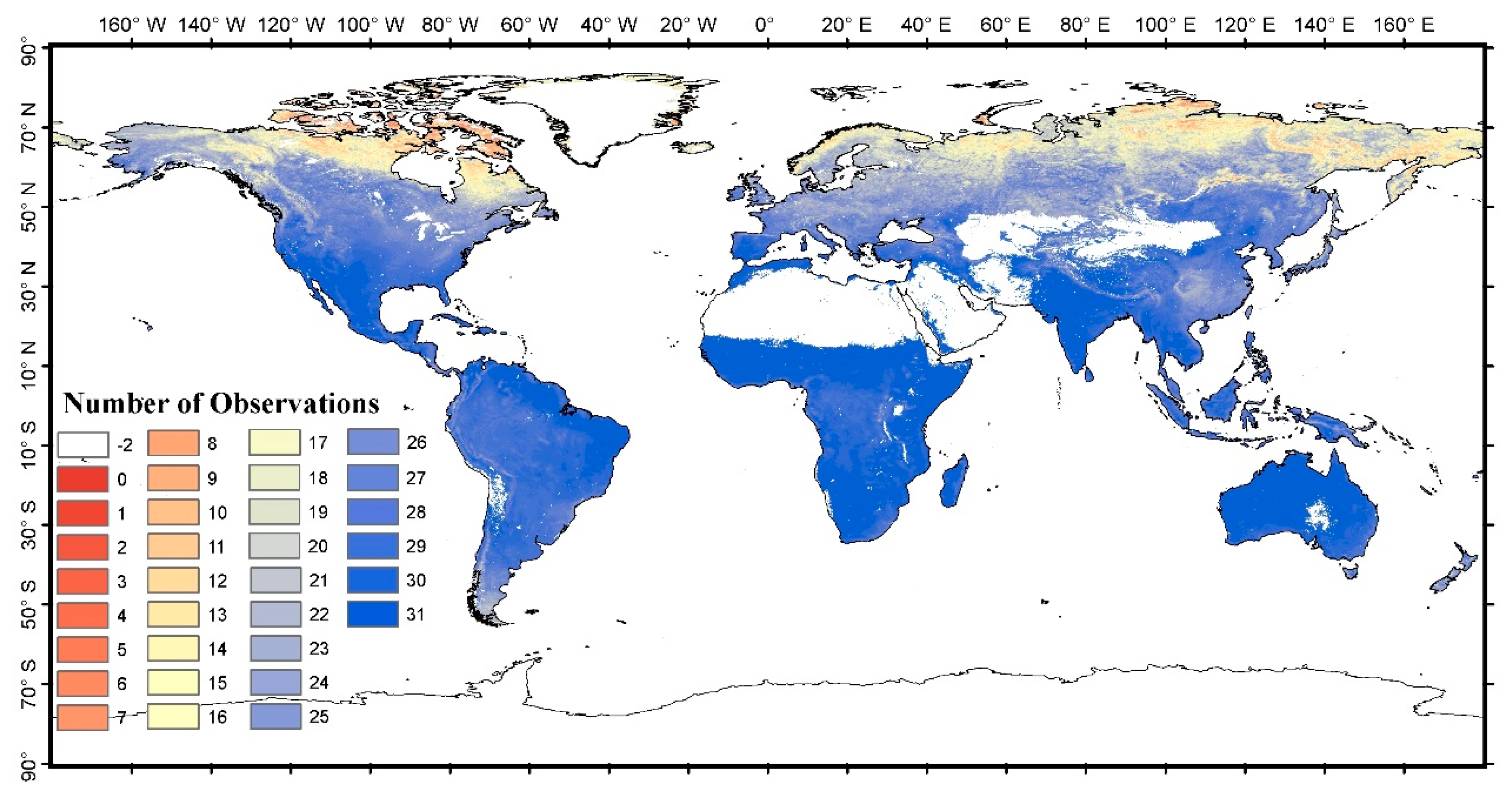
2.8. Number of Observations

We computed the number of observations as a potential source of error in the classification process. This variable was computed as the total daily observations in each month minus the number of days in which each pixel had “No data values” or reflectance equal to or greater than 90% (considered noise). The total number of observations varied throughout the months (28–31 days) and the number of NOAA-AVHRR satellites (1 or 2) that were active that day. An example of this calculus is included in Figure 11. Generally, a higher number of observations were found nearby the Equator, while boreal regions had the lowest.

2.9. Validation

Using Landsat data to validate the product would produce unrealistic estimations of accuracy, considering the large difference in spatial resolution between these two sources of data. In addition, our product was expected to have a low temporal reporting accuracy, as it was built from monthly composites, which would make the comparison with short acquisition periods between two Landsat observations difficult.

For these reasons, a preliminary validation of the FireCCILT10 product was based on comparing the BA estimation of this product with the MCD64A1 for the eight years not used in generating the RF models (2002, 2005, 2010, 2012, 2015, 2016, and 2017). We compared areal estimations of our product with those of MCD64A1 for continental regions [44] by computing the correlation and regression parameters for the eight years between the two datasets.

In addition, we compared our results for the long time series with several national fire perimeters, which are representative of different fire biomes and have a long time series. We included fire perimeters from the Canadian Wildland Fire Information System [52], the state of California [53] and the North Australian Fire Information database [54]. The first two include fire statistics that covered the full time series of our LTDR BA product.

3. Results

3.1. Spatial Patterns

Figure 12 shows the spatial patterns of BA detected by the FireCCILT10 product in relation to the MCD64A1 in 2016. Africa was the most burned continent, especially at the tropical fringes. A total of 74.37% of the whole BA occurred in Africa. MCD64A1 aggregated at 0.05 degrees showed only 2.5% more pixels burned than FireCCILT10, with more detections in the northern latitudes, while FireCCILT10 showed a higher concentration of BA in tropical regions. The main differences between the two products were found in boreal regions and northern South America. In Africa, great similarities were observed, specifically in sites where there was more BA.

According to the continental regions [44], MCD64A1 estimated more BA than FireCCILT10 in each region (

Table 2. Average Burned Area of the FireCCILT10 and MCD64A1 products (2001–2017) in the continental regions. Boreal North America (BONA), Temperate North America (TENA), Central America (CEAM), Northern Hemisphere South America (NHSA), Southern Hemisphere South America (SHSA), Europe (EURO), Middle East (MIDE), Northern Hemisphere Africa (NHAF), Southern Hemisphere Africa (SHAF), Boreal Asia (BOAS), Central Asia (CEAS), Southeast Asia (SEAS), Equatorial Asia (EQAS) and Australia and New Zealand (AUST).

Continental Region	BONA	TENA	CEAM	NHSA	SHSA	EURO	MIDE
MCD64A1 (Mkm2)	0.428	0.478	0.468	0.894	5.002	0.186	0.239
FireCCILT10 (Mkm2)	0.093	0.187	0.201	0.463	3.519	0.102	0.050
Continental Region	NHAF	SHAF	BOAS	CEAS	SEAS	EQAS	AUST
MCD64A1 (Mkm2)	21.917	25.927	1.586	3.417	2.358	0.260	8.702
FireCCILT10 (Mkm2)	20.348	22.984	0.745	1.378	1.948	0.100	5.204

), although they showed similar spatial variability. Southern Hemisphere Africa was the most burned region, followed by Northern Hemisphere Africa. Australia and New Zealand and Southern Hemisphere South America were also greatly affected by fire in both BA products. Europe, the Middle East, and Equatorial Asia were the least burned regions.

The highest discrepancies between the MCD64A1 and the FireCCILT10 were found in boreal regions, where the latter product showed a clear underestimation. This should be related to the low quality observations of the LTDR time series in northern latitude regions, where many months had less than five valid images.

In terms of land cover, the most affected category was tree cover, broadleaved, deciduous, closed to open (15%) with 49.27% of the total burned area, followed by shrubland (25.59%), and rainfed cropland (8.49%).

3.2. Temporal Trends

The FireCCILT10 BA product includes thirty-six years of global BA (1982–2017, excluding 1994). The average yearly BA was 3.12 Mkm², with a maximum burned area of 4.45 Mkm² in 2011 and minimum burned area of 1.74 Mkm² in 1988 (Figure 13). Annual BA estimations from the FireCCILT10 product showed a high inter-annual variability from 1982 to 2000, with more stable trends after 2001 and during the common period with MCD64A1. Decreasing BA at the end of the period (2012–2017) was observed in both products, although it was more evident in FireCCILT10.

Seasonal fire trends were distributed by regions, in particular, the northern hemispheric tropical belt at the end and beginning of the year and the southern hemispheric tropical belt in the middle of the year. Monthly average BA indicated that December and September had the highest values of BA with 0.44 Mkm² and 0.38 Mkm², respectively, and April (0.09 Mkm²) and May (0.10 Mkm²) had the lowest.

3.3. Validation Results

Figure 14 shows the scatterplot of the BA estimations for the MCD64A1 and FireCCILT10 products in the different continental regions. Only the eight common years not used in the training phase were included in this graph. Global correlation was highly significant, although it was highly influenced by the most burned regions (both hemispheres of Tropical Africa). Average estimations for all regions indicate a tendency toward underestimation (18%), according to the slope value. Figure 15 shows the temporal evolution of residuals for the different continents. Residuals are the difference between the MCD64A1 and FireCCILT10 multiplied by the slope of the BA estimations. The larger values corresponded to the most burned regions, with significant underestimation in Australia in 2012 and Southern Hemisphere Africa in 2005 and 2017. A large overestimation was found in the same area in 2010 and, less relevant, in Northern Hemisphere Africa for the same year. Boreal regions and Central Asia showed a consistent underestimation in all validation years.

Comparison of the FireCCILT10 BA estimations and national fire perimeters (Figure 16) showed the limitations of our product, particularly for boreal regions (the example was from Canada), where the fire trends were not well captured, mainly in the pre-MODIS era. For California, the trends were unstable, with a high overestimation in 1992 and underestimation in 2008. The time series had better agreement with the national perimeters after 1998. The FireCCILT10 estimations for the Northern Australia BA were also unstable, with better agreement for the years with lower occurrence. This Australian database only started in 2001 as it is derived from MODIS 250 m data. Unfortunately, there are no fire perimeters for other tropical regions, where our product should produce better agreement than for temperate or boreal regions. The agreements of the national perimeters and the MCD64A1 product were quite reasonable for the three datasets.

4. Discussion

This paper presents the design and prototype processing of a BA algorithm adapted to LTDR data. The final product offers the longest BA time series currently available. Considering the radiometric and spatial limitations of the LTDR data, detecting BA from this data was very challenging, but also attractive for serving the needs of the climate and atmospheric modeling community. The coarse pixel size of LTDR makes the discrimination of the burned signal very complex as a significant proportion of the 0.05° pixels had to be burned to observe significant changes in reflectance or temperature. In fact, existing global BA products based on 250 or 500 m MODIS images have shown great difficulties in discriminating BA in small fire patches or low intense fires [15,17]. These problems are emphasized when working at a much coarser spatial resolution.

Classifying an LTDR pixel as fully burned might have created severe BA overestimation. Therefore, we had to develop a method to convert a binary classification to percentages of BA. We based this analysis on existing BA datasets (MCD64A1) for the common periods, which corrected overestimations, but obviously incorporated the errors of that reference BA dataset.

Another challenge of using LTDR for BA classification is related to the temporal inconsistencies of the middle infrared channel of LTDR. This channel (#3) was changed during the period 2000–2003, moving from the previous 3.7 microns range to an alternative day/night configuration. These changes, plus the lower radiometric stability of this channel, precluded its use for detecting active fires. Active fires are widely used in BA detection [15,17,55] as their strong thermal contrast from the background is much easier to detect than reflectance changes. Consequently, discriminating burned areas without active fire information creates many difficulties in separating BA from other covers with strong temporal changes (seasonal floods, deforestation, cropping, etc.).

Another limitation of the LTDR dataset is the temporal inconsistencies of the reflectance among the satellites [33]. For this reason, different years were used to train the RF models, although they were restricted to the most recent ones, when MODIS BA was available. Considering the seasonal variability of fire impacts, particularly in the Tropics, different RF models were created for each month of the year and assumed similar patterns between the pre- and post-MODIS eras.

The last limitation of the LTDR series regards to the QA inconsistencies: their low quality does not allow the identification of artifacts such as clouds.

The design of the LTDR BA algorithm was based on trying to solve all of these challenges. Composites were used instead of daily images to reduce the impact of clouds, unobserved areas, and artifacts by using the maximum temperature criterion previously tested in other studies [34]. However, compositing potentially reduces the temporal reporting accuracy, as the output composites may have different dates for neighbor pixels.

RF models were selected as they are more robust than other techniques to inconsistencies in input data, while they provide great generalization potential. After several RF test trainings with the original variables, it was decided to generate a synthetic index to facilitate the generalization of the RF models to global BA conditions. In addition, several authors have shown that RF models improve their accuracy with a small number of well-selected and non-redundant input variables [48,56]. The resulting variable (named LBI) is an empirical index, derived from the statistics of burned and unburned pixels, but also based on the experience of previous BA studies [17,23,42,49,55]. This index included red and NIR reflectance, temperature, and some spectral indices. Both the original data and indices considered monthly values and temporal differences. All were normalized using each month’s global statistics to reduce the impact of the temporal instability of the LTDR dataset. RF models were created using the annual variability of the LBI to better discriminate burned areas from other covers that have a strong temporal variation.

As expected, the FireCCILT10 product had lower accuracy values than the other global BA products based on higher resolution sensors. Further efforts are required to improve BA detection, particularly to reduce the impacts of sensor changes in the pre-MODIS era. FireCCILT10 showed good agreement with MCD64A1 at the continental level, although the performance was much higher for tropical than for temperate or boreal regions. Average yearly BA of FireCCILT10 for the common years was lower than MCD64A1 (3.37 Mkm² versus 4.23 Mkm², respectively). In terms of the stability of the temporal series, unrealistic changes between consecutive years were observed in the FireCCILT10 product. The factors that influenced the inter-annual variability were the number of observations, the changes in satellite orbit, and the intercalibration among the AVHRR sensors of different satellites [33].

Future efforts should concentrate on stabilizing the BA temporal series and increasing the sensitivity of the BA product to boreal and temperate regions, where fire occurrence is much less important than in tropical areas. Alternative classification methods (support vector machines, deep learning) will also be tested.

5. Conclusions

FireCCILT10 is the first global BA dataset developed from the LTDR product (v5) and includes the longest time series of BA (1982–2017) currently available.

The algorithm was based on a synthetic index that integrated different input variables to emphasize the burned signal. The BA algorithm was built using RF models and trained with MCD64A1 BA data. Monthly models were created with a set of contrasted years to be more generalized. The probabilities of burning were converted to binary burned maps and then to proportions of burned area by also using the MCD64A1 information for the overlapping period.

The yearly average BA was 3.12 Mkm² in the time series, with Africa being the region with the largest extension of BA (74.37%). 2011 was the most burned year (4.45 Mkm²) and 1988 the least burned (1.74 Mkm²). There were seasonal fire trends according to the different months; December (0.44 Mkm²) and September (0.38 Mkm²) were the most burned periods. The most burned land cover classes around the world and in Africa were tree cover, broadleaved, deciduous, closed to open (15%), shrubland, cropland, and rainfed. Temporal trends of FireCCILT10 and MCD64A1 products were found to be similar at the continental scale, but important differences were found at the national scale, particularly in boreal and temperate regions. Trends had a high inter-annual variability in the pre-MODIS (1982–1999) era and were more stable in the MODIS era (2000–2017). The estimated BA was found to be directly related to the quality of the input LTDR data (particularly the number of observations, the intercalibration among satellites, and the orbital decay of the satellites).

The FireCCILT10 dataset is freely accessible at [57].

References

1. Ciais, P.; Sabine, C.; Bala, G.; Bopp, L.; Brovkin, V.; Canadell, J.; Chhabra, A.; DeFries, R.; Galloway, J.; Heimann, M.; et al. Carbon and other biogeochemical cycles. In Climate Change 2013: The Physical Science Basis. Contribution of Working Group I to the Fifth Assessment Report of the Intergovernmental Panel on Climate Change; Stocker, T.F., Qin, D., Plattner, G.-K., Tignor, M., Allen, S.K., Boschung, J., Nauels, A., Xia, Y., Bex, V., Midgley, P.M., Eds.; Cambridge University Press: Cambridge, UK, 2014; pp. 465–570. [Google Scholar]
2. Bond, W.J.; Woodward, F.I.; Midgley, G.F. The global distribution of ecosystems in a world without fire. New Phytol. 2005, 165, 525–538. [Google Scholar] [CrossRef] [PubMed]
3. Urbanski, S.P.; Hao, W.M.; Baker, S. Chemical composition of wildland fire emissions. Dev. Environ. Sci. 2008, 8, 79–107. [Google Scholar]
4. GCOS. Systematic Observation Requirements for Satellite-Based Products for Climate, 2011 Update; World Meteorological Organization: Geneva, Switzerland, 2011. [Google Scholar]
5. Granier, C.; Bessagnet, B.; Bond, T.; D’Angiola, A.; van Der Gon, H.D.; Frost, G.J.; Heil, A.; Kaiser, J.W.; Kinne, S.; Klimont, Z.; et al. Evolution of anthropogenic and biomass burning emissions of air pollutants at global and regional scales during the 1980–2010 period. Clim. Chang. 2011, 109, 163–190. [Google Scholar] [CrossRef]
6. Ward, D.; Kloster, S.; Mahowald, N.; Rogers, B.; Randerson, J.; Hess, P. The changing radiative forcing of fires: Global model estimates for past, present and future. Atmos. Chem. Phys. 2012, 12, 10857–10886. [Google Scholar] [CrossRef]
7. Hantson, S.; Arneth, A.; Harrison, S.P.; Kelley, D.I.; Prentice, I.C.; Rabin, S.S.; Archibald, S.; Mouillot, F.; Arnold, S.R.; Artaxo, P.; et al. The status and challenge of global fire modelling. Biogeosciences 2016, 13, 3359–3375. [Google Scholar] [CrossRef] [Green Version]
8. Mouillot, F.; Field, C.B. Fire history and the global carbon budget: A 1 degrees × 1 degrees fire history reconstruction for the 20th century. Glob. Chang. Biol. 2005, 11, 398–420. [Google Scholar] [CrossRef]
9. Power, M.J.; Marlon, J.R.; Bartlein, P.J.; Harrison, S.P. Fire history and the global charcoal database: A new tool for hypothesis testing and data exploration. Palaeogeogr. Palaeoclimatol. Palaeoecol. 2010, 291, 52–59. [Google Scholar] [CrossRef]
10. Mouillot, F.; Schultz, M.G.; Yue, C.; Cadule, P.; Tansey, K.; Ciais, P.; Chuvieco, E. Ten years of global burned area products from spaceborne remote sensing—A review: Analysis of user needs and recommendations for future developments. Int. J. Appl. Earth Obs. Geoinf. 2014, 26, 64–79. [Google Scholar] [CrossRef]
11. Grégoire, J.M.; Tansey, K.; Silva, J.M.N. The gba2000 initiative: Developing a global burned area database from spot-vegetation imagery. Int. J. Remote Sens. 2003, 24, 1369–1376. [Google Scholar] [CrossRef]
12. Tansey, K.; Grégoire, J.M.; Defourny, P.; Leigh, R.; Peckel, J.F.; Bogaert, E.V.; Bartholome, J.E. A new, global, multi-annual (2000–2007) burnt area product at 1 km resolution. Geophys. Res. Lett. 2008, 35, L01401. [Google Scholar] [CrossRef]
13. Copernicus Programme. Available online: https://land.copernicus.eu/ (accessed on 1 September 2019).
14. Roy, D.P.; Boschetti, L.; Justice, C.O. The collection 5 modis burned area product—Global evaluation by comparison with the modis active fire product. Remote Sens. Environ. 2008, 112, 3690–3707. [Google Scholar] [CrossRef]
15. Giglio, L.; Boschetti, L.; Roy, D.P.; Humber, M.L.; Justice, C.O. The collection 6 modis burned area mapping algorithm and product. Remote Sens. Environ. 2018, 217, 72–85. [Google Scholar] [CrossRef]
16. Van Der Werf, G.R.; Randerson, J.T.; Giglio, L.; Van Leeuwen, T.T.; Chen, Y.; Rogers, B.M.; Mu, M.; Van Marle, M.J.; Morton, D.C.; Collatz, G.J.; et al. Global fire emissions estimates during 1997–2016. Earth Syst. Sci. Data 2017, 9, 697–720. [Google Scholar] [CrossRef]
17. Chuvieco, E.; Lizundia-Loiola, J.; Pettinari, M.L.; Ramo, R.; Padilla, M.; Tansey, K.; Mouillot, F.; Laurent, P.; Storm, T.; Heil, A. Generation and analysis of a new global burned area product based on modis 250 m reflectance bands and thermal anomalies. Earth Syst. Sci. Data 2018, 10, 2015–2031. [Google Scholar] [CrossRef]
18. Chuvieco, E.; Englefield, P.; Trishchenko, A.P.; Luo, Y. Generation of long time series of burn area maps of the boreal forest from noaa–avhrr composite data. Remote Sens. Environ. 2008, 112, 2381–2396. [Google Scholar] [CrossRef]
19. Kucêra, J.; Yasuoka, Y.; Dye, D.G. Creating a forest fire database for the far east of asia using noaa/avhrr observation. Int. J. Remote Sens. 2005, 26, 2423–2439. [Google Scholar] [CrossRef]
20. Sukhinin, A.I.; French, N.H.F.; Kasischke, E.S.; Hewson, J.H.; Soja, A.J.; Csiszar, I.A.; Hyer, E.J.; Loboda, T.; Conrad, S.G.; Romasko, V.I.; et al. Avhrr-based mapping of fires in Russia: New products for fire management and carbon cycle studies. Remote Sens. Environ. 2004, 93, 546–564. [Google Scholar] [CrossRef]
21. Barbosa, P.M.; Grégoire, J.M.; Pereira, J.M.C. An algorithm for extracting burned areas from time series of avhrr gac data applied at a continental scale. Remote Sens. Environ. 1999, 69, 253–263. [Google Scholar] [CrossRef]
22. Moreno Ruiz, J.A.; Riano, D.; Arbelo, M.; French, N.H.; Ustin, S.L.; Whiting, M.L. Burned area mapping time series in canada (1984–1999) from noaa-avhrr ltdr: A comparison with other remote sensing products and fire perimeters. Remote Sens. Environ. 2012, 117, 407–414. [Google Scholar] [CrossRef]
23. García-Lázaro, J.; Moreno-Ruiz, J.; Riaño, D.; Arbelo, M. Estimation of burned area in the northeastern siberian boreal forest from a long-term data record (ltdr) 1982–2015 time series. Remote Sens. 2018, 10, 940. [Google Scholar] [CrossRef]
24. Riaño, D.; Ruiz, J.A.M.; Isidoro, D.; Ustin, S.L. Global spatial patterns and temporal trends of burned area between 1981 and 2000 using noaa-nasa pathfinder. Glob. Chang. Biol. 2007, 13, 40–50. [Google Scholar] [CrossRef]
25. European Space Agency and Fire_cci Project Team. Available online: https://www.esa-fire-cci.org/ (accessed on 1 September 2019).
26. Pedelty, J.; Devadiga, S.; Masuoka, E.; Brown, M.; Pinzon, J.; Tucker, C.; Vermote, E.; Prince, S.; Nagol, J.; Justice, C.; et al. Generating a long-term land data record from the avhrr and modis instruments. In Proceedings of the 2007 IEEE International Geoscience and Remote Sensing Symposium, Barcelona, Spain, 23–28 July 2007; pp. 1021–1025. [Google Scholar]
27. ESA. Land Cover cci: Algorithm Theoretical Basis Document Version 2; Land_Cover_CCI_ATBDv2_2.3; ESA: Louvain, Belgium, 2013; 191p, Available online: https://www.esa-landcover-cci.org/?q=webfm_send/75 (accessed on 02 September 2019).
28. Padilla, M.; Stehman, S.V.; Hantson, S.; Oliva, P.; Alonso-Canas, I.; Bradley, A.; Tansey, K.; Mota, B.; Pereira, J.M.; Chuvieco, E. Comparing the accuracies of remote sensing global burned area products using stratified random sampling and estimation. Remote Sens. Environ 2015, 160, 114–121. [Google Scholar] [CrossRef] [Green Version]
29. Padilla, M.; Wheeler, J.; Tansey, K. Esa Climate Change Initiative—Fire_cci. D4.1.1 Product Validation Report (pvr). Available online: http://www.esa-fire-cci.org/documents (accessed on 2 September 2019).
30. Myneni, R.B.; Keeling, C.; Tucker, C.J.; Asrar, G.; Nemani, R.R. Increased plant growth in the northern high latitudes from 1981 to 1991. Nature 1997, 386, 698. [Google Scholar] [CrossRef]
31. Horion, S.; Fensholt, R.; Tagesson, T.; Ehammer, A. Using earth observation-based dry season ndvi trends for assessment of changes in tree cover in the sahel. Int. J. Remote Sen. 2014, 35, 2493–2515. [Google Scholar] [CrossRef]
32. Trishchenko, A.P.; Fedosejevs, G.; Li, Z.; Cihlar, J. Trends and uncertainties in thermal calibration of avhrr radiometers onboard noaa-9 to noaa-16. J. Geophys. Res. Atmos. 2002, 107, ACL 17-11–ACL 17-13. [Google Scholar] [CrossRef]
33. Tian, F.; Fensholt, R.; Verbesselt, J.; Grogan, K.; Horion, S.; Wang, Y. Evaluating temporal consistency of long-term global ndvi datasets for trend analysis. Remote Sens. Environ. 2015, 163, 326–340. [Google Scholar] [CrossRef]
34. Chuvieco, E.; Ventura, G.; Martín, M.P.; Gomez, I. Assessment of multitemporal compositing techniques of modis and avhrr images for burned land mapping. Remote Sens. Environ. 2005, 94, 450–462. [Google Scholar] [CrossRef]
35. Rouse, J.W.; Haas, R.W.; Schell, J.A.; Deering, D.H.; Harlan, J.C. Monitoring the Vernal Advancement and Retrogradation (Greenwave effect) of Natural Vegetation; NASA/GSFC: Greenbelt, MD, USA, 1974. [Google Scholar]
36. Simon, M.; Plummer, S.; Fierens, F.; Hoelzemann, J.J.; Arino, O. Burnt area detection at global scale using atsr-2: The globscar products and their qualification. J. Geophys. Res. Atmos. 2004, 109, D14S02. [Google Scholar] [CrossRef]
37. Pinty, B.; Verstraete, M.M. Gemi: A non-linear index to monitor global vegetation from satellites. Vegetatio 1992, 101, 15–20. [Google Scholar] [CrossRef]
38. Martín, M.P.; Chuvieco, E. Cartografía de grandes incendios forestales en la península ibérica a partir de imágenes noaa-avhrr. Ser. Geográfica 1998, 7, 109–128. [Google Scholar]
39. Huete, A.R. A soil-adjusted vegetation index (savi). Remote Sens. Environ. 1988, 25, 295–309. [Google Scholar] [CrossRef]
40. Chuvieco, E.; Martín, M.P.; Palacios, A. Assessment of different spectral indices in the red-near-infrared spectral domain for burned land discrimination. Int. J. Remote Sens. 2002, 23, 5103–5110. [Google Scholar] [CrossRef]
41. McGwire, K.C.; Minor, T.; Fenstermaker, L. Hyperspectral mixture modeling for quantifying sparse vegetation cover in arid environments. Remote Sens. Environ. 2000, 72, 360–374. [Google Scholar] [CrossRef]
42. Barbosa, P.M.; Gregoire, J.-M.; Pereira, J.M.C. Detection of Burned Areas in Africa using A Multitemporal Multithreshold Analysis of NOAA AVHRR GAC Data. In Proceedings of the SPIE, Bellingham, WA, USA, 22–25 September 1997. [Google Scholar]
43. Chuvieco, E.; Mouillot, F.; van der Werf, G.R.; San Miguel, J.; Tanasse, M.; Koutsias, N.; García, M.; Yebra, M.; Padilla, M.; Gitas, I.; et al. Historical background and current developments for mapping burned area from satellite earth observation. Remote Sens. Environ. 2019, 225, 45–64. [Google Scholar] [CrossRef]
44. Giglio, L.; Randerson, J.T.; Werf, G.R. Analysis of daily, monthly, and annual burned area using the fourth generation global fire emissions database (gfed4). J. Geophys. Res. Biogeosci. 2013, 118, 317–328. [Google Scholar] [CrossRef]
45. Rodriguez-Galiano, V.F.; Ghimire, B.; Rogan, J.; Chica-Olmo, M.; Rigol-Sanchez, J.P. An assessment of the effectiveness of a random forest classifier for land-cover classification. ISPRS J. Photogramm. Remote Sens. 2012, 67, 93–104. [Google Scholar] [CrossRef]
46. Pelletier, C.; Valero, S.; Inglada, J.; Champion, N.; Dedieu, G. Assessing the robustness of random forests to map land cover with high resolution satellite image time series over large areas. Remote Sens. Environ. 2016, 187, 156–168. [Google Scholar] [CrossRef]
47. Belgiu, M.; Drăguţ, L. Random forest in remote sensing: A review of applications and future directions. ISPRS J. Photogramm. Remote Sens. 2016, 114, 24–31. [Google Scholar] [CrossRef]
48. Ramo, R.; García, M.; Rodríguez, D.; Chuvieco, E. A data mining approach for global burned area mapping. Int. J. Appl. Earth Obs. Geoinf. 2018, 73, 39–51. [Google Scholar] [CrossRef]
49. Ramo, R.; Chuvieco, E. Developing a random forest algorithm for modis global burned area classification. Remote Sens. 2017, 9, 1193. [Google Scholar] [CrossRef]
50. Long, T.; Zhang, Z.; He, G.; Jiao, W.; Tang, C.; Wu, B.; Zhang, X.; Wang, G.; Yin, R. 30 m resolution global annual burned area mapping based on landsat images and google earth engine. Remote Sens. 2019, 11, 489. [Google Scholar] [CrossRef]
51. Dice, L.R. Measures of the amount of ecologic association between species. Ecology 1945, 26, 297–302. [Google Scholar] [CrossRef]
52. Natural Resources Canada. Available online: cwfis.cfs.nrcan.gc.ca/ha/nfdb (accessed on 1 September 2019).
53. State of California. Available online: frap.fire.ca.gov (accessed on 1 September 2019).
54. North Australia & Rangelands Fire Information. Available online: www.firenorth.org.au/nafi2 (accessed on 1 September 2019).
55. Alonso-Canas, I.; Chuvieco, E. Global burned area mapping from envisat-meris and modis active fire data. Remote Sens. Environ. 2015, 163, 140–152. [Google Scholar] [CrossRef]
56. Dillon, G.K.; Holden, Z.A.; Morgan, P.; Crimmins, M.A.; Heyerdahl, E.K.; Luce, C.H. Both topography and climate affected forest and woodland burn severity in two regions of the western us, 1984 to 2006. Ecosphere 2011, 2, 1–33. [Google Scholar] [CrossRef]
57. European Space Agency and Fire_cci Project Team. Available online: https://geogra.uah.es/fire_cci/ltdr.php (accessed on 1 September 2019).
Figure 1. Flowchart of the methodology to obtain the FireCCILT10 BA product. The method starts with the input data (shown in grey), which are processed and converted into a BA classification. This product is validated independently in the validation step (shown in light orange).
Remotesensing 11 02079 g001
Figure 2. Global and daily data availability of LTDR (v5) in the time series where it was possible to find different problems such as gaps without data (as in 1994 with an eight-month gap or specific gaps in the time series), several daily images with more than one sensor, and corrupt or repeated files.
Remotesensing 11 02079 g002
Figure 3. Evolution of near infrared reflectance (channel 2) in the time series. A pixel in the Sahara Desert was selected to better observe the radiometric stability of the different AVHRR sensors, as this area is very stable throughout time [30,31]. In the shift of the different sensors, the greatest instabilities were shown when new versions of the AVHRR sensor were used such as in 2000 with NOAA 16. N07 to N19 indicate the satellite where the AVHRR was mounted, meaning from the NOAA-7 to the NOAA-19 satellites.
Remotesensing 11 02079 g003
Figure 4. Time series of brightness temperature for channel 3 (3.55–3.93 µm) for a pixel located in the Sahara Desert. The impact of changes related to the daytime configuration of AVHRR3 (1.58–1.64) can be clearly seen between 2000–2003. In 2003, the previous configuration was restored.
Remotesensing 11 02079 g004
Figure 5. Difference between AVHRR2/3 in a Sahara Desert pixel of channel 3 (3.55–3.93 µm). The saturation between AVHRR2/3 was different: AVHRR2 was saturated at 50 °C and AVHRR3 at 63 °C. Therefore, before 2000 (AVHRR2), the data were distributed in a narrower range than after 2000 (AVHRR3). This implies a significant variation between the sensors.
Remotesensing 11 02079 g005
Figure 6. Impact of temporal compositing for the LTDR data. (Left) Daily images acquired on July 18, 2008. (Right) Monthly composite for July 2008 with the unburnable classes removed. In both cases, the RGB color composition used NIR, red, and red reflectances.
Remotesensing 11 02079 g006
Figure 7. Monthly variation (2008) of the LTDR BA Index for an example of the burned area (BA) and unburned area (NBA) pixels. Southern Hemisphere South America (SHSA), Europe (EURO), Northern Hemisphere Africa (NHAF), Southern Hemisphere Africa (SHAF), and Australia and New Zealand (AUST).
Remotesensing 11 02079 g007
Figure 8. LBI values for July 2008. Higher LBI values were observed in the Southern Hemisphere tropical regions, when the dry period occurred.
Remotesensing 11 02079 g008
Figure 9. Representation and composition of the random forest model. Twelve monthly models were created using two variables with the data from eight years.
Remotesensing 11 02079 g009
Figure 10. Calculation of the percentage of Burned Area for the 0.25° cell. The MCD64A1 had 15 pixels classified as burned after aggregating all years during the time series. The LTDR product had 20 pixels classified as burned for the same period. Therefore, each LTDR pixel for this cell was considered to be 75% burned.
Remotesensing 11 02079 g010
Figure 11. Average number of observations per month in the time series. The number of observations shows the number of good observations (without “no data values” or reflectance equal to or higher than 90%).
Remotesensing 11 02079 g011
Figure 12. FireCCILT10 (top) and MCD64A1 (bottom) burned area in 2016.
Remotesensing 11 02079 g012
Figure 13. BA annual trends of the MCD64A1 and FireCCILT10 BA products.
Remotesensing 11 02079 g013
Figure 14. BA estimations of the MCD64A1 and FireCCILT10 products for the continental regions.
Remotesensing 11 02079 g014
Figure 15. Temporal variability of residuals for the different continental regions (for acronyms see the caption of Table 2).
Remotesensing 11 02079 g015
Figure 16. Comparison of the BA trends between FireCCILT10, MCD64A1, and the national fire perimeters: Canada (top), California (center), and Northern Australia (bottom). Note that the vertical scale is quite different among sites, as they have very different fire occurrences.
Remotesensing 11 02079 g016