Article

Improved Empirical Coefficients for Estimating Water Vapor Weighted Mean Temperature over Europe for GNSS Applications

Faculty of Civil and Environmental Engineering, Gdansk University of Technology, 80-233 Gdansk, Poland
*
Author to whom correspondence should be addressed.
Remote Sens. 2019, 11(17), 1995; https://doi.org/10.3390/rs11171995
Submission received: 20 July 2019 / Revised: 14 August 2019 / Accepted: 20 August 2019 / Published: 23 August 2019
(This article belongs to the Special Issue Feature Papers for Section Atmosphere Remote Sensing)

Abstract

:
Development of the so-called global navigation satellite system (GNSS) meteorology is based on the possibility of determining a precipitable water vapor (PWV) from a GNSS zenith wet delay (ZWD). Conversion of ZWD to the PWV requires application of water vapor weighted mean temperature ( T m ) measurements, which can be done using a surface temperature ( T s ) and its linear dependency to the T m . In this study we analyzed up to 24 years (1994–2018) of data from 49 radio-sounding (RS) stations over Europe to determine reliable coefficients of the T m T s relationship. Their accuracy was verified using 109 RS stations. The analysis showed that for most of the stations, there are visible differences between coefficients estimated for the time of day and night. Consequently, the ETm4 model containing coefficients determined four times a day is presented. For hours other than the primary synoptic hours, linear interpolation was used. However, since this approach was not enough in some cases, we applied the dependence of T m T s coefficients on the time of day using a polynomial (ETmPoly model). This resulted in accuracy at the level of 2.8 ± 0.3 K. We also conducted an analysis of the impact of this model on the PWV GNSS. Analysis showed that differences in PWV reached 0.8 mm compared to other commonly used models.

1. Introduction

Earth’s atmosphere affects electromagnetic global navigation satellite system (GNSS) signals by delaying their propagation. While the ionosphere influence can be reduced using dual-frequency measurements, the delay caused by the troposphere has to be estimated during the precise positioning process. Tropospheric delay is usually expressed in the zenith direction (zenith tropospheric delay, ZTD) and it describes the total impact of neutral atmosphere on the GNSS signals. Therefore, ZTD contains delays caused by the hydrostatic (zenith hydrostatic delay, ZHD) and the wet (zenith wet delay, ZWD) part of the troposphere. Both ZHD and ZWD depend on the meteorological parameters and, consequently, changes in these parameters over time. ZHD is correlated with changes of air pressure and temperature, while ZWD depends on the amount of water vapor in the atmosphere.
The sensitivity of the ZWD parameter to the water vapor content variation has triggered the development of the so-called GNSS meteorology. It is based on the possibility of converting the ZWD to precipitable water vapor (PWV) [1], which describes the total content of water vapor in the air column above a GNSS antenna. Short-term monitoring of the water vapor variations is an important element in monitoring and studying of rapid changes of weather conditions [2,3,4]. On the other hand, estimation of the PWV long-term parameters can be used as part of investigation of the climate change [5,6,7]. Vertical PWV variations can be obtained via GNSS tomography [8]. Although this approach enables to estimate accurate humidity distribution through troposphere, it requires delivering of temperature profiles, using dense network of GNSS receivers and complex calculations. PWV can be also calculated based on the ZTD derived from GNSS processing and various external meteorological parameters. Temperature and air pressure profiles are used to estimate ZHD, which is necessary to obtain ZWD. In turn, profiles of temperature and water vapor pressure are required to calculate water vapor weighted mean temperature ( T m ), which takes part in the conversion from ZWD to PWV. In situ measurements of the profiles can be done using radiosonde or microwave radiometers. Unfortunately, the vast majority of GNSS stations are not collocated with such instruments. Thus, it is not possible to obtain the required meteorological data. Therefore, it is necessary to apply some simplifications. ZHD can be accurately modeled using total air pressure at the GNSS antenna location [9], while T m can be obtained based on the linear relationship with the surface temperature ( T s ): T m = a T S + b . This relationship (henceforth named T m T s ) was firstly proposed by Bevis et al. [1]. In their model, the a (slope) and b (intercept) coefficients were calculated on the basis of 8712 radiosonde profiles made on 13 U.S. stations over a two-year period. They determined the values of the coefficients at 0.72 and 70.2 for a and b , respectively, with the root mean square error (RMSE) at the level of 4.74 K. Braun and Van Hove [10] used, based on a personal communication from Michael Bevis, revised version of these coefficients. Based on the profiles derived from nearly globally distributed radio-soundings stations, updated coefficients values were estimated: a = 0.668 and b = 85.63 .
A linear regression analysis of the radiosonde profiles was also conducted by Mendes and Langley [11] who based on the data from stations located between 62°S to 83°N proposed that the following coefficients can be used: a = 0.789 and b = 50.4 . Ross and Rosefeld [12] found that geographical localization may affect the reliability of the T m T s model and have proposed to use the nonlinear function ( T m = 3.402 × 10 6 T s 3 + 196.05 ) for stations located at higher latitudes. Consequently, regional models have started to be developed. Here, Emardson et al. [13] can be mentioned, who have proposed to use a model which included information about time of the year for the Scandinavia region, or Solbrig et al. [14], who have used simple T m T s but estimated specifically for the territory of Germany. Despite the fact that they only included data from Germany, they obtained results ( a = 0.77 , b = 54.7 ) similar to those presented by Mendes and Langley on a global scale. The optimization of the T m T s for the specific area was also undertaken by, e.g., Liu et al. for Taiwan [15], Baltink et al. for the Netherlands [16], Bokoye et al. for Canada [17], Suresh et al. for India [18], Sappucci for Brazil [19], Mekik and Deniz for Turkey [20], Liu et al. for China [21], or Zhang et al. for Tahiti [22]. These works show the importance of developing accurate spatio-temporal models of T m . Simultaneously, new global coefficients were also modeled. Based on the data from the numeric model, Schueler et al. [23] proposed three approaches: Harmonics, which took into account the day of year and seasonal variations of T m , a linear T m T s , and a combined periodic/linear assumption. Yao et al. [24] have proposed a station location (latitude, longitude, and elevation) and season-dependent coefficients for the T m T s linear relation. Lan et al. [25] proposed a gridded model with 2° × 2.5° window size to deliver the site-accurate a and b coefficients, while Yao et al. [26] developed a globally applicable global weighted mean temperature (GWMT) model which considered annual cycle, as well as semi-annual and diurnal variation of T m sourced from the Global Geodetic Observing System (GGOS).
All so far developed models have some advantages and limitations. Local models are best suited to the prevailing weather conditions occurring over a given region, while global models can be used on larger scale. On the other hand, in the case of global models, the coverage of radio-sounding (RS) stations is not uniform. This evokes the need to accept a compromise between model accuracy and global availability or the need to source data from weather models, not in situ observations. The numerical weather models, in turn, contain the average values of meteorological parameters, which can cause deterioration of the results. Until now, there is a lack of a regional model that could be used across the European continent with high accuracy. In this paper, we focus on a regional model of the T m T s relationship, developed exclusively on the basis of in situ measurements. In total, we used observations from 109 RS stations evenly distributed throughout Europe to deliver and validate reliable coefficients of the T m T s . More details about the employed data are given in Section 2 together with a description of the methodology. The accuracy of the selected models is assessed in Section 3. The process of estimation of new coefficients is presented in Section 4, while the results are described and discussed in Section 5.

2. Data and Methodology

ZTD, together with the station coordinates, is a direct product of GNSS processing. It contains hydrostatic (ZHD) and wet components (ZWD):
Z T D = Z H D + Z W D .
ZWD is strictly correlated to the amount of water vapor in the atmosphere and can be converted to PWV by:
P W V =   Π T m ZWD ,
where Π is a dimensionless quantity dependent on T m :
Π 1 = 10 8 × R v K 3 / T m + K 2 ,
where R v is the specific gas constant of water vapor (461.5 J/kg K), and:
K 2 = K 2 K 1 M w M d 22.1   k / h P a ,
where K 1 ,   K 2 ,   K 3 denotes air refractivity parameters. Here, we applied the “best average” values estimated by Ruger [27], equal to 77.689 ± 0.0094 K/hPa, 71.295 ± 1.3 K/hPa, and 3.75463 × 10⁵ ± 0.0076 K2/hPa, respectively. M w =   18.0151 and M d =   28.9644 are the molar masses of wet and dry air expressed in g/mol.
We have stated that T m can be obtained by vertical integration of the temperature in the atmosphere and requires measurements from a sounding station or a microwave radiometer, or data from an accurate and validated numerical weather model. The other way is to use the linear relationship with the T s . To estimate T m T s coefficients, it is necessary to know both values at the station location. In this study, observations from 109 RS stations located in Europe were used (Figure 1). Values of T s were derived directly from the measurements while T m were calculated by vertical integration of the temperature ( T ) and water vapor pressure ( P w ) profiles:
T m = h 0 h m a x P w / T P w / T 2 d h ,
where h 0 is a station altitude and h m a x denotes the maximum height of the atmospheric profile. We used only profiles made up to at least 8 km.
Thus obtained time series of T m and T s were divided into two groups. The first of them contained stations which have been working since 1994 to 2018, collected at least 80% of observations, and were free from visible shifts and significant gaps (henceforth named estimation group). This group consists of 49 stations and constitutes a basis for estimation new coefficients of T m T s (Figure 1, the red triangles) using linear regression. To ensure independent verification of our results, we selected the second group containing 60 RS stations (Figure 1, the light violet circles). These stations (henceforth named external group) have at least 2 years of observations and together with the estimation group were used as an external indicator of the accuracy of all coefficients shown in this paper. All observations were obtained from Earth System Research Laboratory (ESRL) database and were checked before analysis. Incomplete or too low (below 8 km) profiles as well as abnormal recorded values were removed from further processing.
In Section 5, we provide the impact of the new estimated coefficients on the PWV. Therefore, we had to extract ZWD from Equation (1). To this end, we used the Saastamoinen hydrostatic model [9] and surface meteorological parameters derived from the ERA5 model [28] and interpolated at the locations of the stations [29]. As we focus on PWV differences, this approach was acceptable.

3. Accuracy of the Existing T m T s Coefficients

Here, we present the assessment of the accuracy of the T m T s coefficients that can be adopted in Europe. We took into consideration only these models which were estimated based on the in situ observations. In the described analysis, all 109 RS stations presented in Figure 1 were used. For each of them the T m values were estimated using Equation (5). They were compared to the T m values calculated from the relationship with T s and various coefficients. Obtained differences have allowed for an assessment which coefficients provide better accuracy and if this accuracy is evenly distributed over the entire area.
We decided to consider coefficients developed by Bevis et al. [1] (henceforth named Bevis coefficients), since they are still one of the most commonly used. Moreover, their revised versions [10] (BevisRev coefficients) as well as values presented by Mendes and Langley [11] (Mendes coefficients) and Solbrig [14] (Solbrig coefficients) were taken into account. 
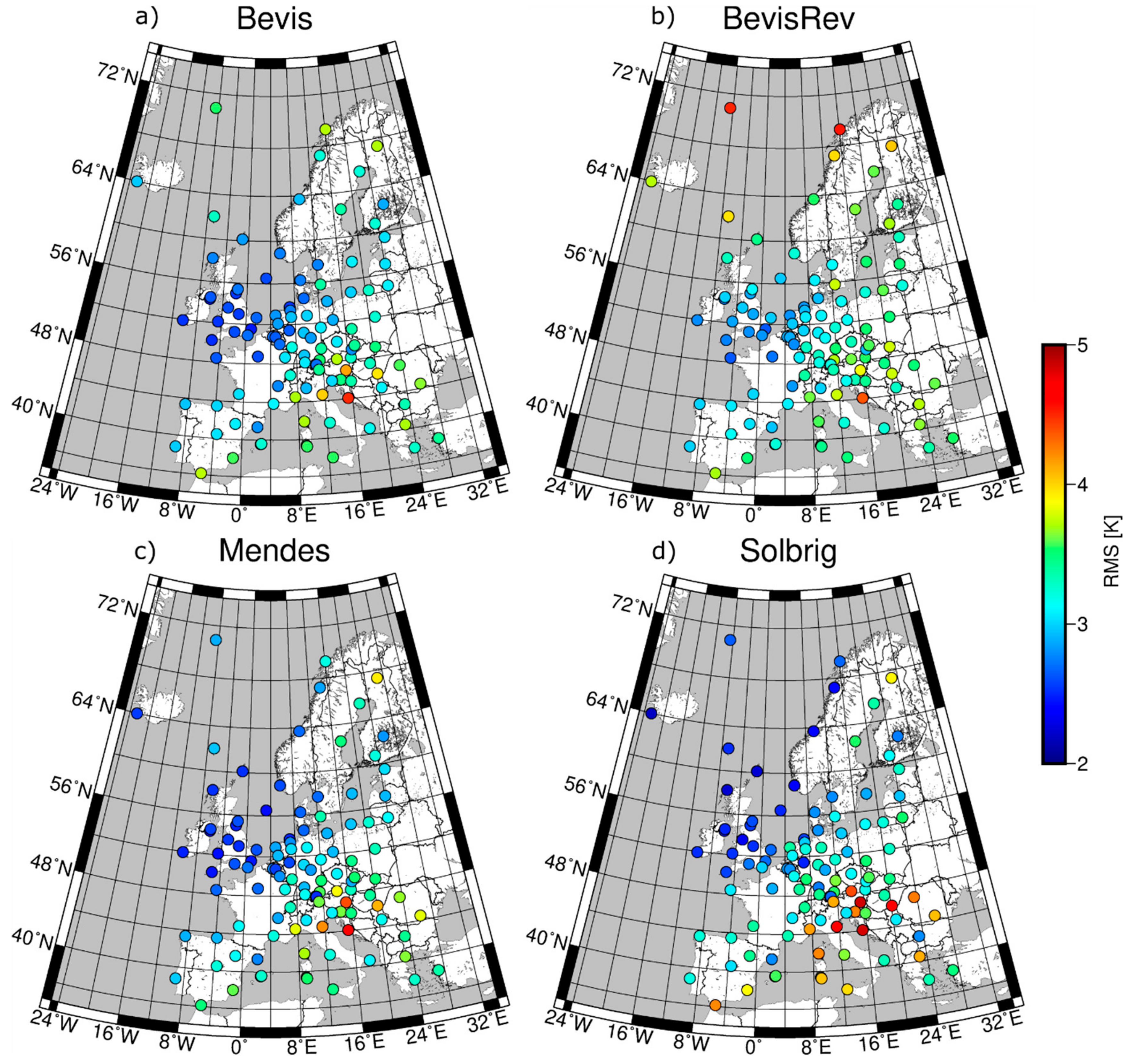
Figure 2 presents the RMSE values for each of the analyzed station and set of coefficients. Using Bevis coefficients, we achieved mean RMSE value at the level of 3.1 ± 0.4 K. As it is seen in Figure 2a, the distribution of RMSE for the individual stations is not homogeneous. The greatest consistency can be found in the north-east area, where for most of the stations the RMSE value is below 3.0 K. This may result from the fact that these stations are located in the temperate oceanic climate zone for which the Atlantic Ocean has a smoothing effect. Similar results can be found when BevisRev coefficients were used (Figure 2b). In this case the mean RMSE was at the level 3.3 ± 0.4 K. These slightly poorer results are probably caused by the spatial distribution of stations used for coefficients estimation (regional in Bevis and global in BevisRev). Application of Mendes coefficients (Figure 2c) did not bring significant difference in results—the mean RMSE value was 3.1 ± 0.5 K. Interesting results were obtained for T m values estimated based on Solbrig coefficients (Figure 2d). Although the coefficients were estimated only for Germany, they can be used for stations located in almost all of Europe, especially the northern part. The obtained accuracy did not diverge significantly from others. The mean RMSE for this solution was 3.2 ± 0.6 K. In this case, the RMSE is affected by poor results obtained for stations located in the Mediterranean area. It is also worth to notice here, as opposed to the expectations, that the stations located in Germany are not characterized by higher accuracy. Summary of the provided results is given in Table 1.
Although part of the stations is in a very good agreement with the T m values obtained by the way of direct measurement, the limitations of these models are also clear. This motivated us to reanalyze RS data from Europe and to verify whether it is possible to estimate coefficients with higher accuracy.

4. Estimation of the New T m T s Coefficients

In the first approach, the T m T s coefficients were estimated using the same method as in case of the above described studies. The T m and T s data from all stations belonging to the estimation group were analyzed in one common process, in which a linear regression was conducted to the whole dataset consisting of 967,277 records. As a result, the coefficients (named ETm) of the T m T s were estimated at 0.7440 ± 0.0004 and 62.84 ± 0.10, for a and b , respectively, with RMSE equal 3.0 K.
The second approach was preceded by an investigation of the relationship between time-varying T m and T s . The possible dependency between T m T s coefficients and the time of day were investigated, e.g., by Mekik and Deniz [19]. In their study, they proved that the differences in RMSE values obtained based on coefficients estimated during day and night are not significant, amounting to about 0.2 K, for RS stations located on the Turkish territory. To verify whether such dependency occur at European stations or not, we estimated T m T s 
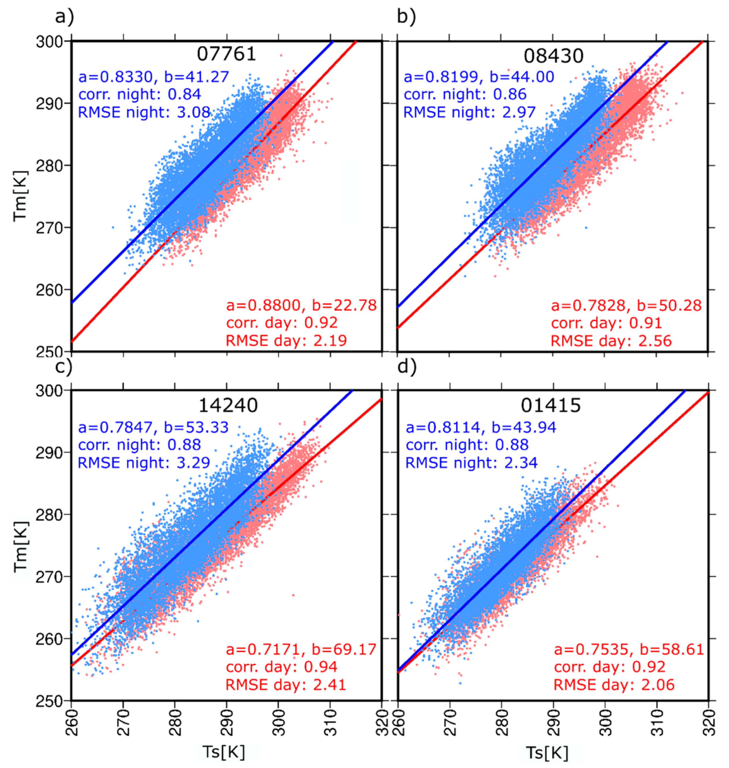
coefficients for two separated synoptic hours: At 00:00 and 12:00 UTC. We found clear differences between the T m T s (Figure 3a–c) estimated during the night (higher RMSE values) and the day (lower RMSE values). In the case of some stations, the RMSE between night and day drops from 3.08 K to 2.19 K, 2.97 K to 2.56 K, and from 3.29 K to 2.41 K for 07761, 08430, and 14240 station, respectively. Only for a few RS stations, the obtained differences were less significant, e.g., 01415 for which RMSE dropped from 2.34 K to 2.06 K (Figure 3d).
The fact that the linear regression coefficients show dependencies on the time of day prompted us to include this fact into the estimation of the new T m T s model. In this approach, observations from the 00:00 and 12:00 UTC collected from all stations belonging to the estimation group were analyzed separately. We obtained the following coefficients for daytime: a = 0.7430 ± 0.004 and b = 61.84 ± 0.13, and for nighttime: a = 0.8436 ± 0.0006 and b = 35.88 ± 0.17. These coefficients, named ETm2, were estimated with RMSE of 2.46 K and 2.91 K, respectively, for the day and the night. It is seen that the obtained RMSE are lower than in case of ETm coefficients, which proves that ETm2 ensures a better fit for the linear model.
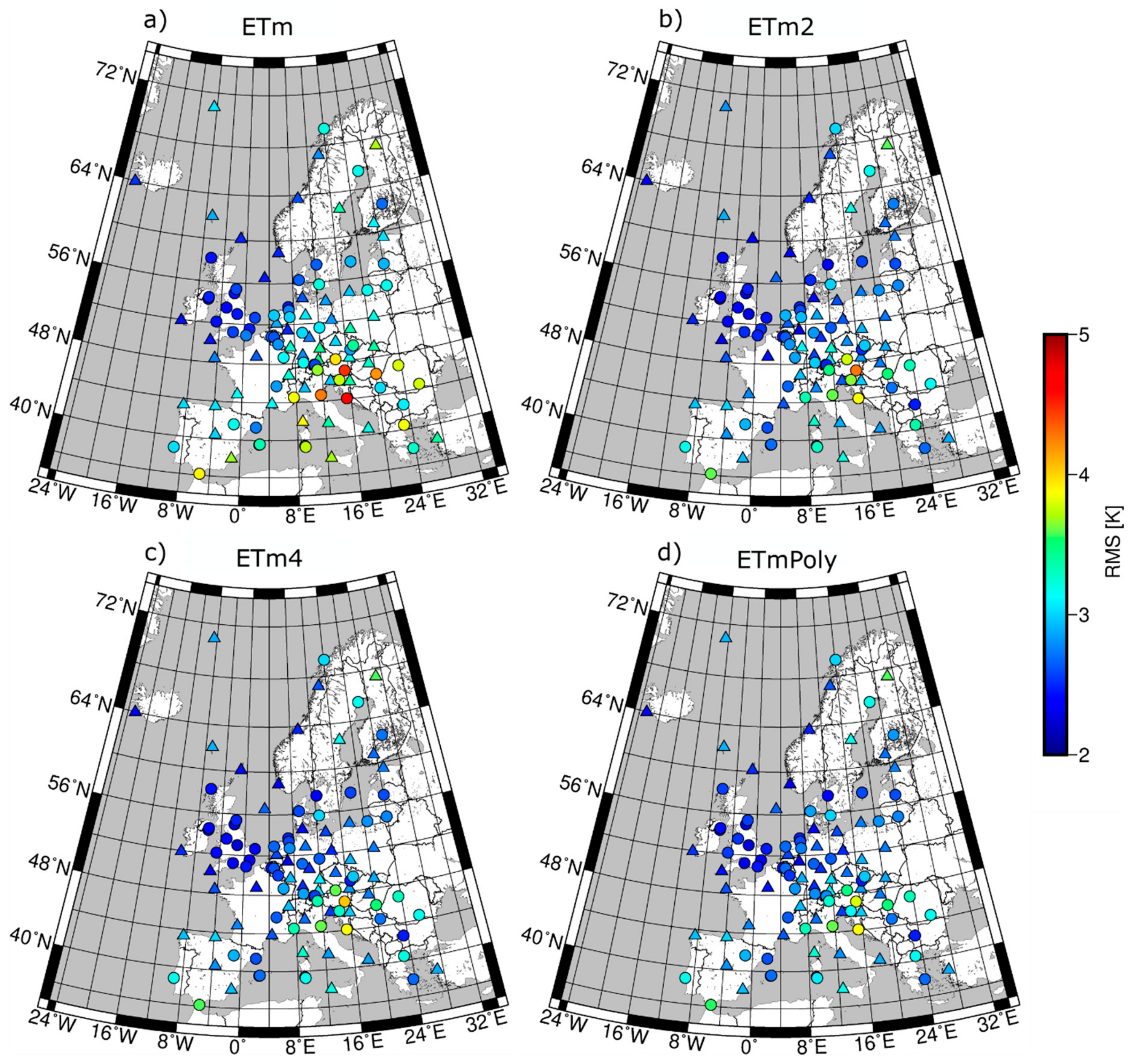
Many RS stations had observations performed also at additional hours, mostly at 06:00 and 18:00 UTC. This fact allowed for an estimation of linear regression coefficients (ETm4) also for these terms. As a result, we have obtained four coefficients of T m T s which are presented in Table 2 together with RMSE. It can be seen that the uncertainties of estimated coefficients at 06:00 and 18:00 have higher values. This is due to the fact of using fewer stations for calculation than on the other terms. Nonetheless, the differences between the coefficients are significantly higher than their uncertainties. Determination the coefficients for several terms in a day can increase the T m accuracy by making the simple T m T s formula time dependent. This will cause the coefficients to be interpolated at a specific time of a day.

5. Results and Discussion

In this section we provide results of validation of obtained coefficients. To this end, in situ measurements from all RS stations were used. Then, we considered the impact of our computed coefficients on PWV calculation at both RS and GNSS stations.

5.1. Accuracy of the New T m T s Coefficients

The accuracy of the presented T m T s coefficients was evaluated in the same way as previously described and expressed by RMSE values. As a reference the T m values obtained directly from RS observations were adopted. In Figure 4, the RMS values obtained for each RS station are presented. The triangles denote stations on the basis of which the coefficients were estimated. Furthermore, an external verification was done by the stations marked by the circles. For the coefficients estimated for different terms of a day (ETm2 and ETm4) we made linear interpolation to obtain values for a given hour of measurement.
The mean RMSE of the T m values calculated using ETm coefficients amounts 3.1 ± 0.5 K. As can be noticed (Figure 4a), the distribution of the RMS value for individual stations is close to those obtained for Bevis and Mendes coefficients. North-eastern Europe shows the higher consistency between estimated and measured T m value, while the Mediterranean area is affected by larger discrepancies between these values. Stations with the poorest accuracy are 14430 (Zadar–Zemunik, Croatia), 16144 (S. Pietro Capofiume Molin, Italy), and 11240 (Graz, Austria). A higher accuracy was obtained when the ETm2 coefficients were used. In this case, the RMSE was at the level of 2.8 ± 0.4 K. In contrast to the ETm, in ETm2 (Figure 4b) there is no inferior fit between measured and estimated parameters in the Mediterranean region. The use of the ETm4 coefficients resulted in the mean RMSE at the level of 2.8 ± 0.4 (Figure 4c). Although, at first sight, these results do not significantly vary from the ETm2 results, it is worth to notice that stations with the poorest (so far) accuracy have improved their results, especially station 11240 (Graz, Austria) (4.4 K to 4.1 K).
The application of linear interpolation to obtain values of coefficients at the specific epoch may introduce some uncertainties because in reality T m changes between four primary synoptic hours may not have a linear nature. Thus, we decided to express daily changes of a and b values using polynomial function. For this purpose, T m T s coefficients were estimated for each epoch when the total number of the RS observations was over 20,000. Then, we fitted polynomials of different degrees. Results are presented in Figure 5. Generally, all polynomials are well fitted in points where the observations were performed (Figure 5, black dots). Therefore, the average RMSE values calculated at all stations are very similar. The difference is visible in detailed comparison of the RS stations which performed measurements at other epochs, e.g., 11240 (Graz, Austria). For this station, the RMSE obtained using fifth degree polynomials (3.7 K) was better by about 0.1 K and 0.5 K then the results obtained using fourth and third degrees, respectively. Application of the sixth degree polynomial coefficients gives worse accuracy represented by the higher average RMSE value of about 0.2 ± 0.2 K (maximum 1.4 K) with comparison to the fifth degree polynomial. We assumed that those fifth degree coefficients allow accurate description of the time-varying T m T s coefficients (named ETmPoly):
a = 10.07 t 5 + 23.95 t 4 19.08 t 3 + 5.998 t 2 0.7914 t + 0.8436 , b = 2985 t 5 7200 t 4 + 5882 t 3 1923 t 2 + 256.8 t + 35.87 ,
where t is a UTC time of the observation, expressed as a fraction of the day.
The results achieved using ETmPoly coefficients are characterized, in general, by an accuracy equal to 2.8 ± 0.3 K (Figure 4d). Most of the stations show similar results to those obtained with ETm4. The 91% of the stations are characterized by differences smaller than 0.1 K and 80% of the stations had differences smaller than 0.05 K. However, we noticed that the highest differences occurred, again, for 11240 station (Graz, Austria), which RMSE decreased from 4.1 K (ETm4) to 3.7 K (ETmPoly). This station has practically no observations at primary synoptic hours (00:00, 06:00, 12:00, and 18:00 UTC), and most of the data concerns hours between 02:00 and 04:00 UTC. Thus, although application of coefficients from the ETm4 model makes it possible to estimate T m , the final accuracy suffers from the lack of observation at primary synoptic hours for which model ETm4 suits the best. Therefore, limitations of the linear interpolation of the ETm4 coefficients and benefits of introducing the non-linear ETmPoly model are easy to seen at this station.

5.2. Impact of the New Coefficients on the PWV Estimated at RS Stations

Here, an assessment of the impact of the new T m T s coefficients on the PWV estimation at RS stations is shown. The analysis was conducted for the ETmPoly, since these coefficients provide the highhest accuracy. PWV calculated using the Bevis coefficients are also shown as a comparison. Both series of PWV were calculated using ZWD and T s obtained at RS stations and Equations (2) and (3). Then, we compared them to the in situ measurements of PWV. Figure 6 presents the RMS for Bevis (left) and ETmPoly (right) coefficients for each of analyzed RS station. In general, the ETmPoly model is characterized by the higher accuracy in southern Europe, the slightly higher in central Europe, and similar in northern Europe, compared to Bevis model.
The above results were obtained for the entire period. Therefore, they represent the average differences and some remarkable details are not visible. In Figure 7, we present PWV differences for selected RS stations and for a representative time span. We selected stations from the areas where the differences between ETmPoly and Bevis were highest. It can be seen that characteristics of the presented variations differ. For station 15614 (Sofia, Bulgaria) a small bias, in the amount of 0.1 mm, is visible for the entire period. However, in the case of station 16144 (S. Pietro Capofiume Molin, Italy), the differences were determined by the season. In winter, the PWV obtained using ETmPoly and Bevis coefficients are almost the same, while during the summer months they are shifted by 0.2 mm. It is worth to notice that for both stations the ETmPoly solution gives more accurate results than the Bevis model.

5.3. Impact of the New Coefficients on the PWV Estimated at GNSS Stations

PWV can be calculated based on GNSS ZWD data which, in contrast to RS data, can be characterized by a much higher frequency of measurements. Here, we show an assessment of the impact of the ETmPoly coefficients on the PWV obtained from hourly ZWD values. Dataset contains ZTD values for 27 GNSS stations belonging to the EUREF Permanent Network (EPN). Tropospheric parameters were estimated using precise point positioning (PPP) method with global mapping function (GMF) [30]. Used data were described in detail in our previous study [29]. Hourly ZTD for each station was converted to the PWV according to the described methodology in Section 2.
Figure 8 shows PWV differences for selected stations. For the stations located at the southern part of the Europe, e.g., EBRE, SFER, or MEDI, the differences exceed ±0.5 mm and for the WTZR station reached 0.8 mm. For stations located at the northern part of the Europe, e.g., KIRU, the differences are smaller and contain usually in the range of ±0.2 mm. These discrepancies result from two reasons. Firstly, it is related to the accuracy of the model coefficients, which was discussed above. Secondly, it is associated with the resolution of the data. In case of GNSS technique, we usually deal with much higher data frequency than in the case of RS measurements. We assumed that the ETmPoly coefficients are linked to more accurate results than the Bevis coefficients. This results from the fact, that for the RS stations which collected observation on different terms than the 00:00, 06:00, 12:00, and 18:00 UTC, the ETmPoly allowed to get the highest accuracy of the T m values, which was described on the basis of 11240 (Graz, Austria) station.
Like in the case of PWV estimated on the basis of RS data (Figure 7), also in the case of GNSS PWV, an increase in the discrepancy between ETMPoly and Bevis solutions took place during the summer months. To verify the spread of these differences depending on the season, we calculated the STD of the differences obtained during December/January/February (DJF) and June/July/August (JJA) seasons. The differences between GNSS PWV estimated using ETmPoly and Bevis are smaller during the DJF (Figure 9a) than during the JJA (Figure 9b) season. Moreover, the discrepancies between the results for individual stations are less significant in this case. Generally, the STDs for DJF are in a range from 0.02 mm to 0.08 mm, with slightly higher values for stations located along the coastal area, compared to the stations located at the continental part of Europe. In JJA, STDs of the differences are between 0.08 mm to 0.22 mm (WARE station) with slightly lower values for stations located at the northern part of Europe. The only exception of this is the GRAS station, which despite the location in the southern part of the continent is characterized by low STD value. This station, however, is also located at the highest altitude (1319 m) from all analyzed cases. Therefore, the smaller humidity fluctuations at this altitude, as well as at the northern part of Europe during the JJA and continental part of Europe during the DJF, supports the determination of similar T m values for both models.

6. Conclusions

This paper presents a comparative analysis of the existing T m T s linear coefficients together with the development of a new form. In total, 109 RS stations over Europe were used to access and validate the accuracy of the T m estimation. Firstly, the Bevis, BevisRev, Mendes, and Solbrig coefficients were examined by comparing T m time series to the in situ measurements derived from RS stations. This indicated that Bevis and Mendes have similar accuracy and spatial distribution of the obtained results. The mean RMSE were 3.1 ± 0.4 K and 3.1 ± 0.5 K, respectively. In both cases, the highest consistency between the estimated and the observed data was found in north-western Europe, while the worst results were seen for the south-east. Similar results for north-western stations were found for the Solbrig coefficients. In other cases, significantly worse results were achieved. The T m estimation using BevisRev coefficients, which is Bevis global revision, was characterized by a mean RMSE at the level of 3.3 ± 0.4 K. Although this model represents a similar distribution of the results, in general, it did not achieve RMSE values as low as in the case of previous models (especially in the north-east area). In addition, stations located at the highest latitudes were represented by much lower accuracy. This is probably a consequence of using low latitude stations and stations from the southern hemisphere for coefficient estimation.
The coefficients we propose were estimated based on 49 RS stations over that were continuously operating for at least 20 years. In total, almost 970,000 records were used to estimate the T m T s coefficients following three different approaches: (i) All observations were used simultaneously to estimate one set of coefficients (ETm), (ii) two set of coefficients were estimated based on a separate calculation of observations only from 0 and 12 hours (ETm2), and (iii) the coefficients were estimated at four (00:00, 06:00, 12:00, 18:00) synoptic hours (ETm4). The determination the coefficients several times a day allowed us to perform an interpolation between terms to increase the T m determination accuracy. We showed that an application of even a simple linear interpolation brings tangible benefits especially for the measurements not performed at four primary synoptic hours. This might be exemplified by differences in T m RMSE between ETm and ETm4 models. For 101 out of 109 RS stations, we noted a reduction in RMSE value. Its mean value was 0.3 K and the highest reached up to 0.8 K (16546, Piras, Italy).
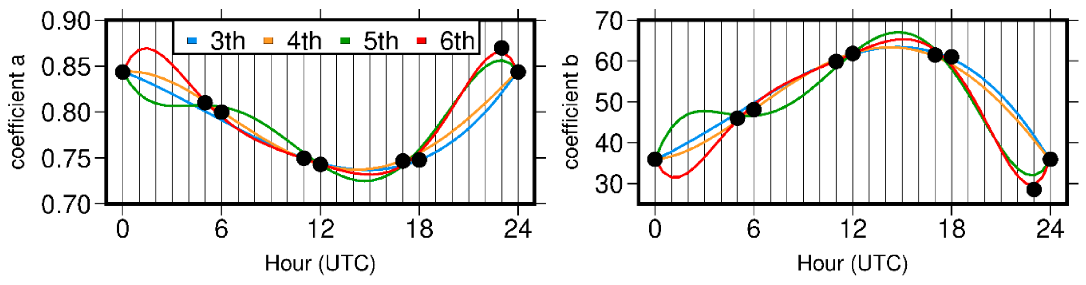
As a complement to the above approaches, we decided to apply a five-degree polynomial fitting instead of a linear interpolation to estimate a and b coefficients for a specific epoch during daytime (ETmPoly). Although this model is based on the exact same set of data as ETm4, we noticed some differences between the obtained results. Despite the fact that the mean RMSE of T m for these two models is the same (2.8 K), the STD was reduced from 0.4 K to 0.3 K. The highest differences between ETm4 and ETmPoly were found for stations which have observations out of primary synoptic hours. Here, the 11240 (Graz, Austria) station, for which RMSE was reduced by 0.4 K, can be mentioned.
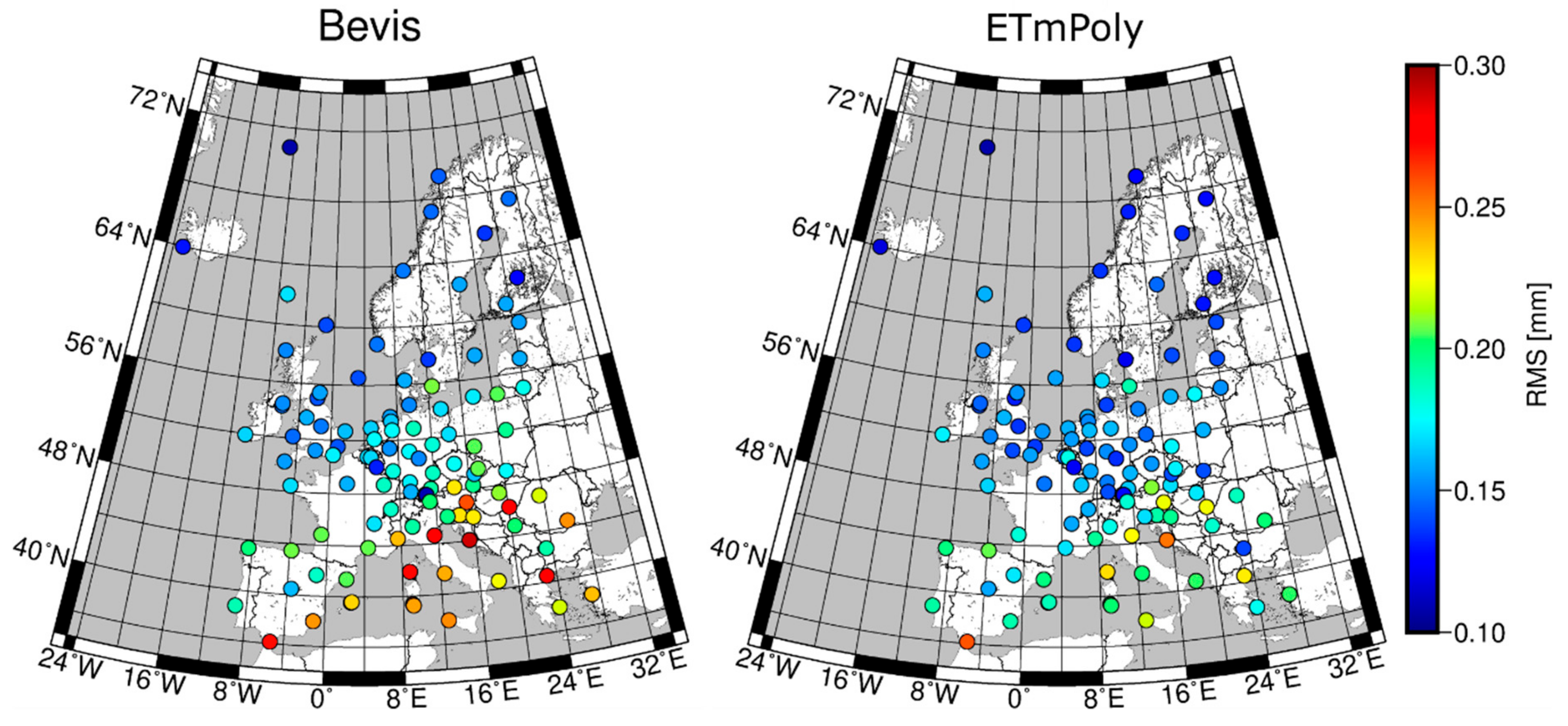
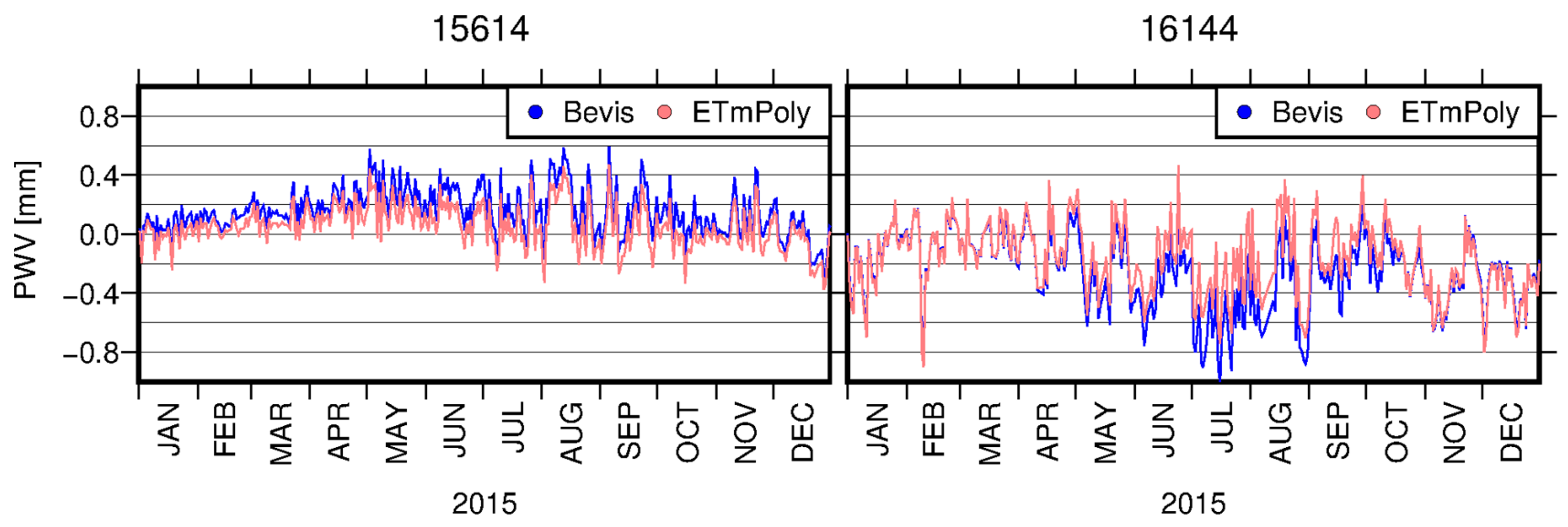
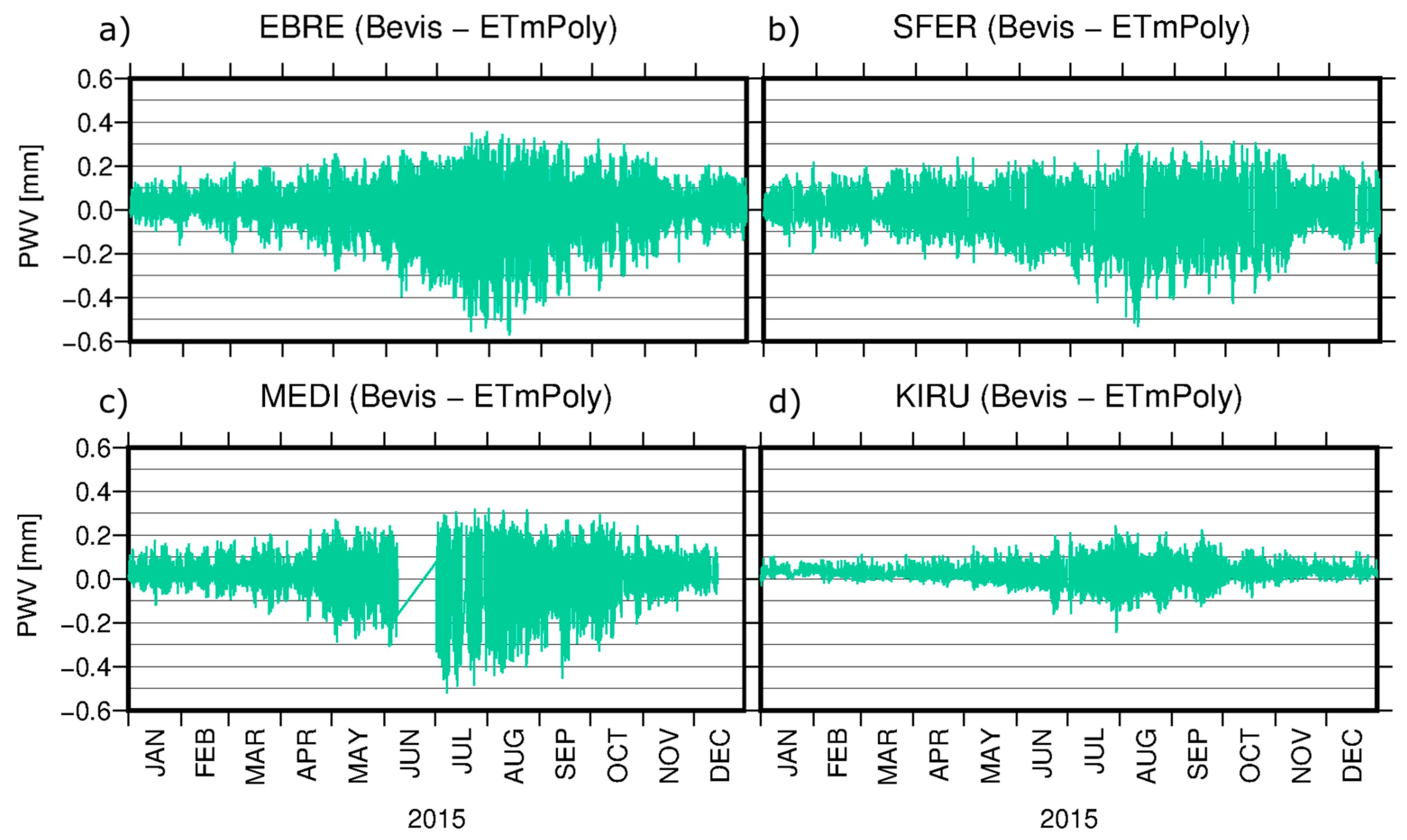
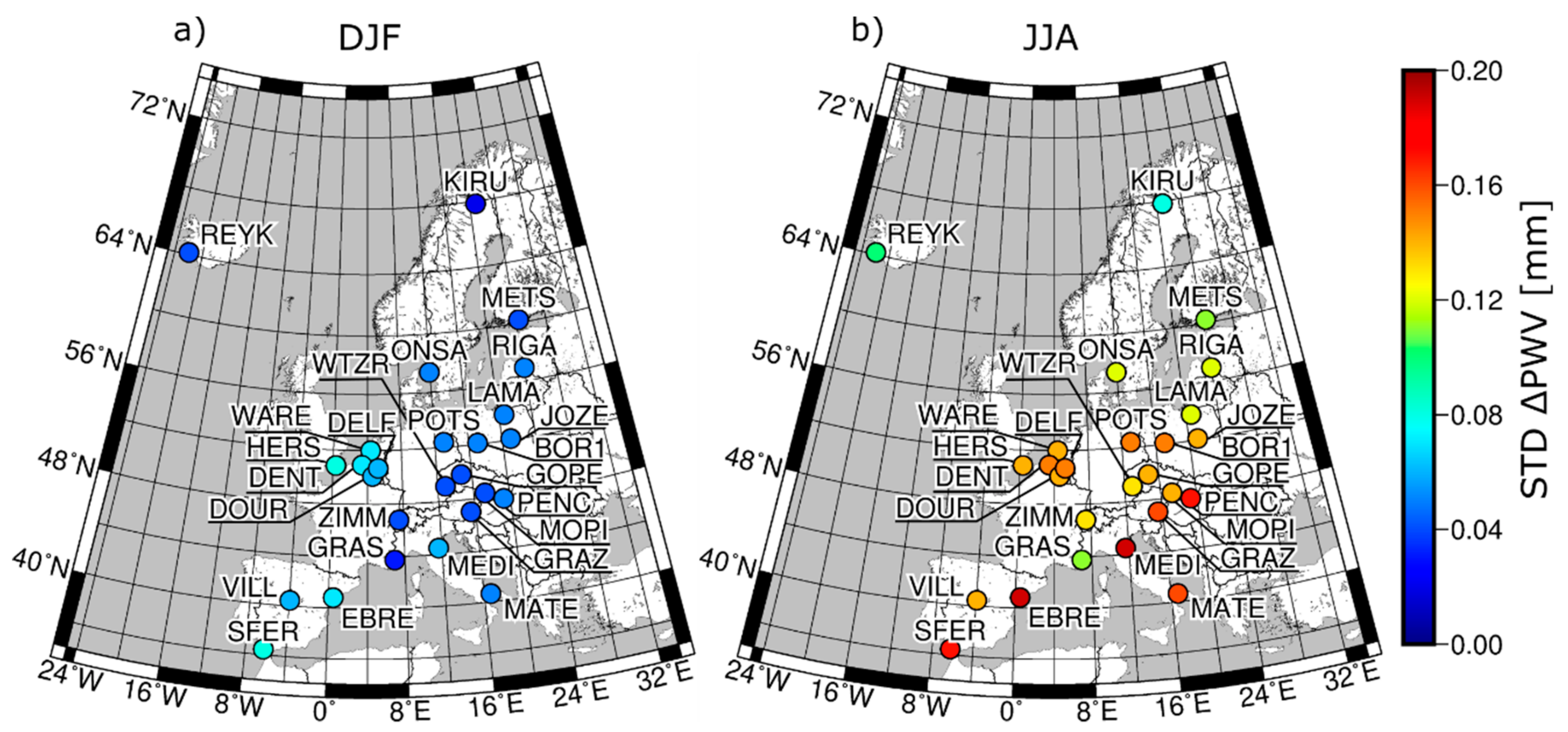
Each of the introduced models containing values of time-varying a and b coefficients represents higher accuracy than the Bevis model. For ETm2, ETm4, and ETmPoly we achieved accuracy at the level of 2.8 ± 0.4 K, 2.8 ± 0.4 K, and 2.8 ± 0.3 K, respectively, while in the case of Bevis model it was 3.1 ± 0.4. In addition to the RMSE, differences between the analyzed approaches can be found during estimation of the PWV value, especially based on GNSS data. We showed that although mean values of differences between, e.g., Bevis and ETmPoly coefficients may not be significant, applying these two models to the data with high temporal resolution results in discrepancies in PWV values up to 0.8 mm.
The most reliable results were obtained using ETmPoly coefficients. This is due to the fact that in addition to time-varying a and b coefficients, this model does not assume a linear character of the changes between main synoptic terms. Taking into account the daily variability of T m T s coefficients during the day by fitting the polynomial bring benefits and is especially important in GNSS meteorology, where time resolution of the observations is much higher than in case of RS.

Author Contributions

Conceptualization, Z.B. and G.N.; methodology, Z.B. and G.N.; validation, Z.B.; formal analysis, Z.B. and G.N.; investigation, Z.B.; resources, G.N.; writing—original draft preparation, Z.B.; writing—review and editing, G.N.; visualization, Z.B.

Funding

This research was funded by the Faculty of Civil and Environmental Engineering of Gdansk University of Technology statutory research funds.

Acknowledgments

Calculations were carried out at the Academic Computer Centre in Gdansk. The authors would like to thank Earth System Research Laboratory (ESRL) database for providing radio-sounding data.

Conflicts of Interest

The authors declare no conflict of interest.

References

  1. Bevis, M.; Businger, S.; Herring, A.T.; Rocken, C.; Anthes, R.A.; Ware, R.H. GPS meteorology: Remote sensing of atmospheric water vapor using the global positioning system. J. Geophys. Res. 1992, 97, 15787–15801. [Google Scholar] [CrossRef]
  2. Guerova, G.; Jones, J.; Douša, J.; Dick, G.; de Haan, S.; Pottiaux, E.; Bock, O.; Pacione, R.; Elgered, G.; Vedel, H.; et al. Review of the state of the art and future prospects of the ground-based GNSS meteorology in Europe. Atmos. Meas. Tech. 2016, 9, 5385–5406. [Google Scholar] [CrossRef] [Green Version]
  3. Priego, E.; Jones, J.; Porres, M.J.; Seco, A. Monitoring water vapour with GNSS during a heavy rainfall event in the Spanish Mediterranean area. Geomat. Nat. Hazards Risk 2017, 8, 282–294. [Google Scholar] [CrossRef]
  4. Nykiel, G.; Figurski, M.; Baldysz, Z. Analysis of GNSS sensed precipitable water vapour and tropospheric gradients during the derecho event in Poland of 11th August 2017. J. Atmos. Sol. Terr. Phys. 2019. [Google Scholar] [CrossRef]
  5. Gradinarsky, L.P.; Johansson, J.M.; Bouma, H.R.; Scherneck, H.G.; Elgered, G. Climate monitoring using GPS. Phys. Chem. Earth 2002, 27, 225–340. [Google Scholar] [CrossRef]
  6. Nilsson, T.; Elgered, G. Long-term trends in the atmospheric water vapor content estimated from groundbased GPS data. J. Geophys. Res.-Atmos. 2008, 113, D19101. [Google Scholar] [CrossRef]
  7. Bianchi, C.E.; Mendoza, L.P.O.; Fernández, L.I.; Natali, M.P.; Meza, A.M.; Moirano, J.F. Multi-year GNSS monitoring of atmospheric IWV over Central and South America for climate studies. Ann. Geophys. 2016, 34, 623–639. [Google Scholar] [CrossRef] [Green Version]
  8. Flores, A.; Ruffini, G.; Rius, A. 4D tropospheric tomography using GPS slant wet delays. Ann. Geophys. 2000, 18, 223–234. [Google Scholar] [CrossRef]
  9. Saastamoinen, J. Atmospheric Correction for the Troposphere and Stratosphere in Ranging Satellites. In The Use of Artificial Satellites for Geodesy; Geophysical Monograph Series; American Geophysical Union: Washington, DC, USA, 1972; pp. 247–251. [Google Scholar] [CrossRef]
  10. Braun, J.J.; Van Hove, T. Recent Improvements in the Retrieval of Precipitable Water Vapor. In Proceedings of the 18th International Technical Meeting of the Satellite Division of The Institute of Navigation (ION GNSS 2005), Long Beach, CA, USA, 13–16 September 2005; pp. 298–301. [Google Scholar]
  11. Mendes, V.B.; Langley, R.B. Tropospheric zenith delay prediction accuracy for high-precision GPS positioning and navigation. Navigation 1999, 46, 25–34. [Google Scholar] [CrossRef]
  12. Ross, R.J.; Rosenfeld, S. Estimating mean weighted temperature of the atmosphere for Global Positioning System. J. Geophys. Res. 1997, 102, 21719–21730. [Google Scholar] [CrossRef]
  13. Emardson, T.R.; Elgered, G.; Johansson, J.M. Three months of continuous monitoring of atmospheric water vapour with a network of Global Positioning System receivers. J. Geophys. Res. 1998, 103, 1807–1820. [Google Scholar] [CrossRef]
  14. Solbrig, P. Untersuchungen uber die Nutzung numerischer Wettermodelle zur Wasserdampfbestimmung mit Hilfe des Global Positioning Systems. Ph.D. Thesis, Institute of Geodesy and Navigation, University FAF Munich, Munich, Germany, 2000. [Google Scholar]
  15. Liou, Y.; Teng, Y.; Van Hove, T.; Liljegren, J.C. Comparison of precipitable water observations in the near tropics by GPS, microwave radiometer, and radiosondes. J. Appl. Meteorol. 2001, 40, 5–15. [Google Scholar] [CrossRef]
  16. Baltink, H.K.; Van Der Marel, H.; Van Der Hoeven, A.G.A. Integrated atmospheric water vapour estimates from a regional GPS network. J. Geophys. Res. 2002, 107, ACL 3-1–ACL 3-8. [Google Scholar] [CrossRef]
  17. Bokoye, A.I.; Royer, A.; O’Neill, N.T.; Cliché, P.; McArthur, L.J.B.; Teillet, P.M.; Thériault, J.M. Multisensor analysis of integrated atmospheric water vapour over Canada and Alaska. J. Geophys. Res. 2003, 108, 15–21. [Google Scholar] [CrossRef]
  18. Suresh Raju, C.; Saha, K.; Thampi, B.V.; Parameswaran, K. Empirical model for mean temperature for Indian zone and estimation of precipitable water vapour from ground based GPS measurements. Ann. Geophys. 2007, 25, 1935–1948. [Google Scholar] [CrossRef]
  19. Sapucci, L.F. Evaluation of modeling water-vapour-weighted mean tropospheric temperature for GNSS-integrated water vapour estimates in Brazil. J. Appl. Meteorol. Clim. 2014, 53, 715–730. [Google Scholar] [CrossRef]
  20. Mekik, C.; Deniz, I. Modelling and validation of the weighted mean temperature for Turkey. Meteorol. Appl. 2017, 24, 92–100. [Google Scholar] [CrossRef]
  21. Liu, J.; Yao, Y.; Sang, J. A new weighted mean temperature model in China. Adv. Space Res. 2018, 61, 402–412. [Google Scholar] [CrossRef]
  22. Zhang, F.; Barriot, J.-P.; Xu, G.; Yeh, T.-K. Metrology Assessment of the Accuracy of Precipitable Water Vapor Estimates from GPS Data Acquisition in Tropical Areas: The Tahiti Case. Remote Sens. 2018, 10, 758. [Google Scholar] [CrossRef]
  23. Schueler, T.; Posfay, A.; Hein, G.W.; Biberger, R. A Global Analysis of the Mean Atmospheric Temperature for GPS Water Vapor Estimation. In Proceedings of the 14th International Technical Meeting of the Satellite Division of The Institute of Navigation (ION GPS 2001), Salt Lake City, UT, USA, 11–14 September 2001; pp. 2476–2489. [Google Scholar]
  24. Yao, Y.; Zhu, S.; Yue, S. A globally applicable, season-specific model for estimating the weighted mean temperature of the atmosphere. J. Geod. 2012, 86, 1125–1135. [Google Scholar] [CrossRef]
  25. Lan, Z.; Zhang, B.; Geng, Y. Establishment and analysis of global gridded Tm–Ts relationship model. Geod. Geodyn. 2016, 7, 101–107. [Google Scholar] [CrossRef]
  26. Yao, Y.; Zhang, B.; Xu, C.; Chen, J. Analysis of the global Tm–Ts correlation and establishment of the latitude-related linear model. Chin. Sci. Bull. 2014, 59, 2340–2347. [Google Scholar] [CrossRef]
  27. Rüger, J.M. Refractive Index Formulae for Radio Waves. In Proceedings of the FIG XXII International Congress, Washington, DC, USA, 19–26 April 2002. [Google Scholar]
  28. Copernicus Climate Change Service (C3S). ERA5: Fifth Generation of ECMWF Atmospheric Reanalyses of the Global Climate. Copernicus Climate Change Service Climate Data Store (CDS). 2017. Available online: https://confluence.ecmwf.int/display/CKB/ERA5+data+documentation (accessed on 20 July 2019).
  29. Baldysz, Z.; Nykiel, G.; Figurski, M.; Araszkiewicz, A. Assessment of the impact of GNSS processing strategies on the long-term parameters of 20 years IWV time series. Remote Sens. 2018, 10, 496. [Google Scholar] [CrossRef]
  30. Boehm, J.; Niell, A.; Tregoning, P.; Schuh, H. Global mapping function (GMF): A new empirical mapping function based on numerical weather model data. Geophys. Res. Lett. 2006, 33, L07304. [Google Scholar] [CrossRef]
Figure 1. Distribution of the radio-sounding (RS) stations used in the study. The red triangles denote stations from the estimation group, whereas the light violet circles denote stations from the external group. The station number is assigned to the station from the estimation group.
Remotesensing 11 01995 g001
Figure 2. RMSE of differences between direct T m measurements and T m calculated using T s and the following coefficients of linear relationship: Bevis (a), BevisRev (b), Mendes (c), Solbrig (d). The dots indicate the location of 109 RS station, while their colors denote RMSE values.
Remotesensing 11 01995 g002
Figure 3. Correlation and T m T s coefficients for selected RS stations: 07761 (Ajaccio, France) (a), 08430 (Murcia, Spain) (b), 14240 (Zagreb Maksimir, Croatia) (c), and 01415 (Stavanger Sola, Norway) (d). The light blue and light pink dots represent observations at 00:00 and 12:00 UTC, respectively. Fitted lines are shown using blue (night) and red (day) lines. Linear regression coefficients ( a and b ), correlation coefficient (corr.) and RMSE for each case are also shown.
Remotesensing 11 01995 g003
Figure 4. RMS values of T m estimated using ETm (a), ETm2 (b), ETm4 (c), and ETmPoly (d) coefficients. RMSE calculated in reference to the in situ measurements performed at RS stations in a period since 1996 to the end of 2018. The circles and the triangles represent RS stations belonging to estimation and external groups, respectively.
Remotesensing 11 01995 g004
Figure 5. Results of fitting different degree polynomials into T m T s linear regression coefficients: a (left) and b (right). Color of the line denotes degree of the polynomial: 3rd—blue, 4th—orange, 5th—green, 6th—red.
Remotesensing 11 01995 g005
Figure 6. RMS values of the precipitable water vapor (PWV) estimated using Bevis (left) and ETmPoly (right) coefficients. The PWV derived from RS profiles were adopted as a reference.
Remotesensing 11 01995 g006
Figure 7. Differences between PWV estimated using Bevis (blue) and ETmPoly (pink) coefficients and PWV obtained directly from the RS measurements, for 15614 (left) and 16144 (right) RS stations.
Remotesensing 11 01995 g007
Figure 8. Differences between PWV values estimated using Bevis and ETmPoly coefficients for EBRE (a), SFER (b), MEDI (c), and KIRU (d) GNSS stations.
Remotesensing 11 01995 g008
Figure 9. Standard deviations of differences between global navigation satellite system (GNSS) PWV values estimated using Bevis and ETmPoly coefficients for the seasons: (a) December/January/February (DJA) and (b) June/July/August (JJA).
Remotesensing 11 01995 g009
Table 1. Average root mean square error (RMSE) ( R M S E ¯ ) of the analyzed coefficients calculated based on 109 RS stations.
T m = a T s + b
Coefficientsab R M S E ¯
Bevis0.7270.23.1 ± 0.4
BevisRev0.66885.633.3 ± 0.4
Mendes0.78950.43.1 ± 0.5
Solbrig0.7754.73.2 ± 0.6
Table 2. Summary of the estimated T m T s coefficients.
T m T s   Coefficients
NameHours (UTC) a b R M S E ¯ Number of Observations
ETmall available0.7440 ± 0.000462.84 ± 0.103.02967 277
ETm200:000.8436 ± 0.000635.88 ± 0.172.91391 401
12:000.7430 ± 0.000461.84 ± 0.132.46381 106
ETm400:000.8436 ± 0.000635.88 ± 0.172.91391 401
06:000.7997 ± 0.001448.07 ± 0.402.9526 160
12:000.7430 ± 0.000461.84 ± 0.132.46381 106
18:000.7478 ± 0.001161.00 ± 0.312.4324 862

