Remote Sensing of Environmental Changes in Cold Regions: Methods, Achievements and Challenges

 ,
,  ,
,  ,
,  , ,
, , 
Abstract
1. Introduction
2. Principles and Methods
2.1. Remote Sensing of Ice
2.1.1. Glacier Mass and Movement
2.1.2. Lake Ice Cover
2.2. Remote Sensing of Snow
2.2.1. Snow Cover Area
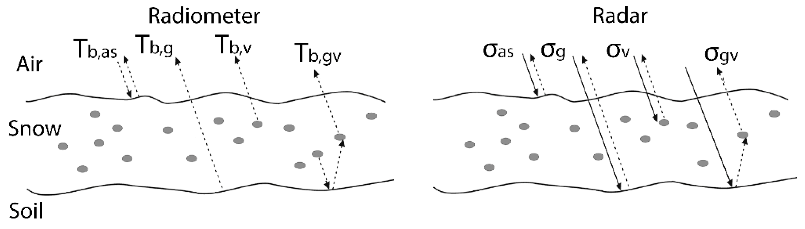
2.2.2. Snow Water Equivalent
2.3. Remote Sensing of Frozen Soil
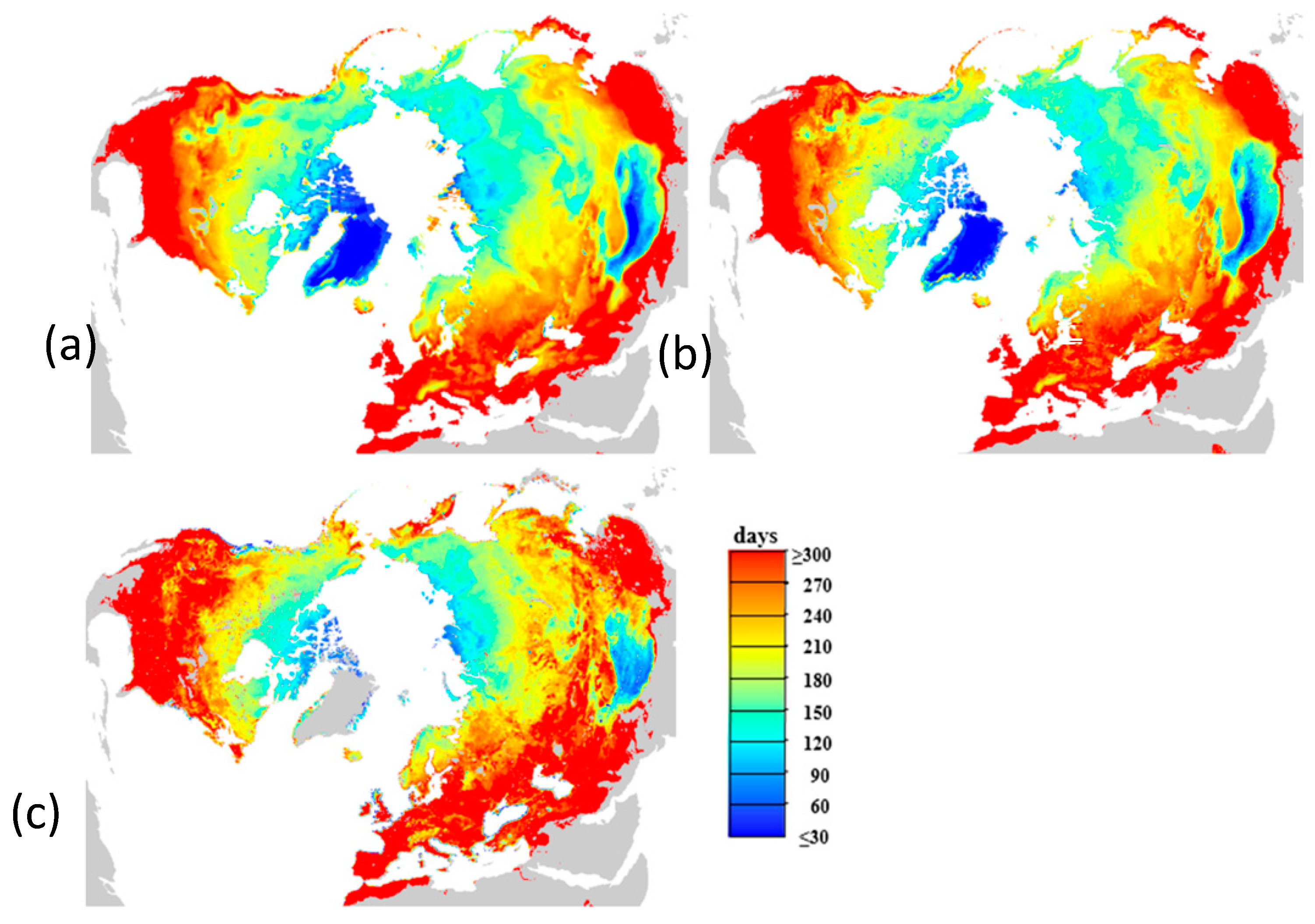
2.3.1. Landscape Freeze/Thaw States
2.3.2. Surface Deformation
2.4. Remote Sensing of Water Bodies
2.5. Remote Sensing of Terrestrial Ecosystems
2.5.1. Vegetation Mapping
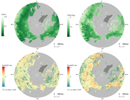
2.5.2. Vegetation Growth and Photosynthetic Carbon Assimilation
3. Changes and Trends
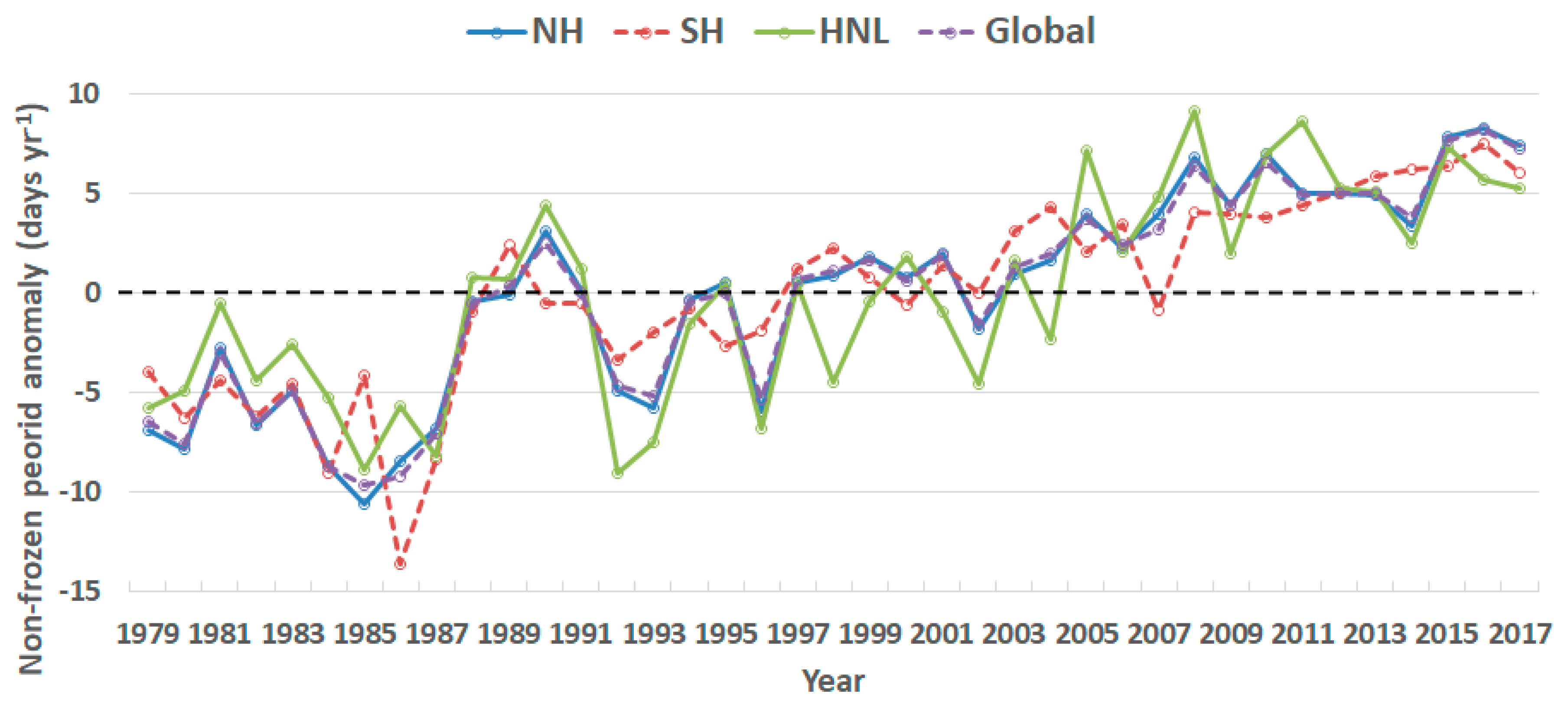
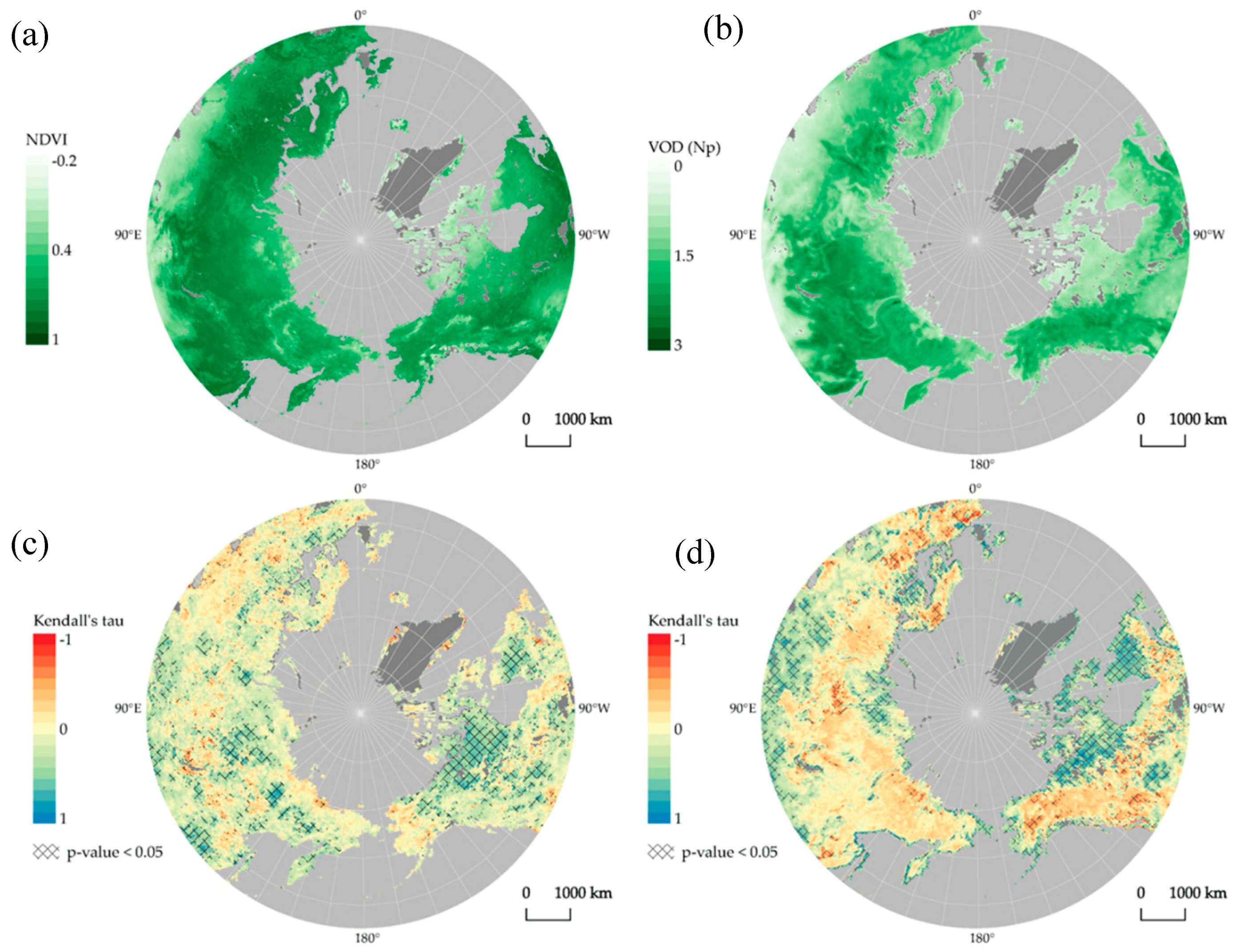
3.1. Northern High Latitudes
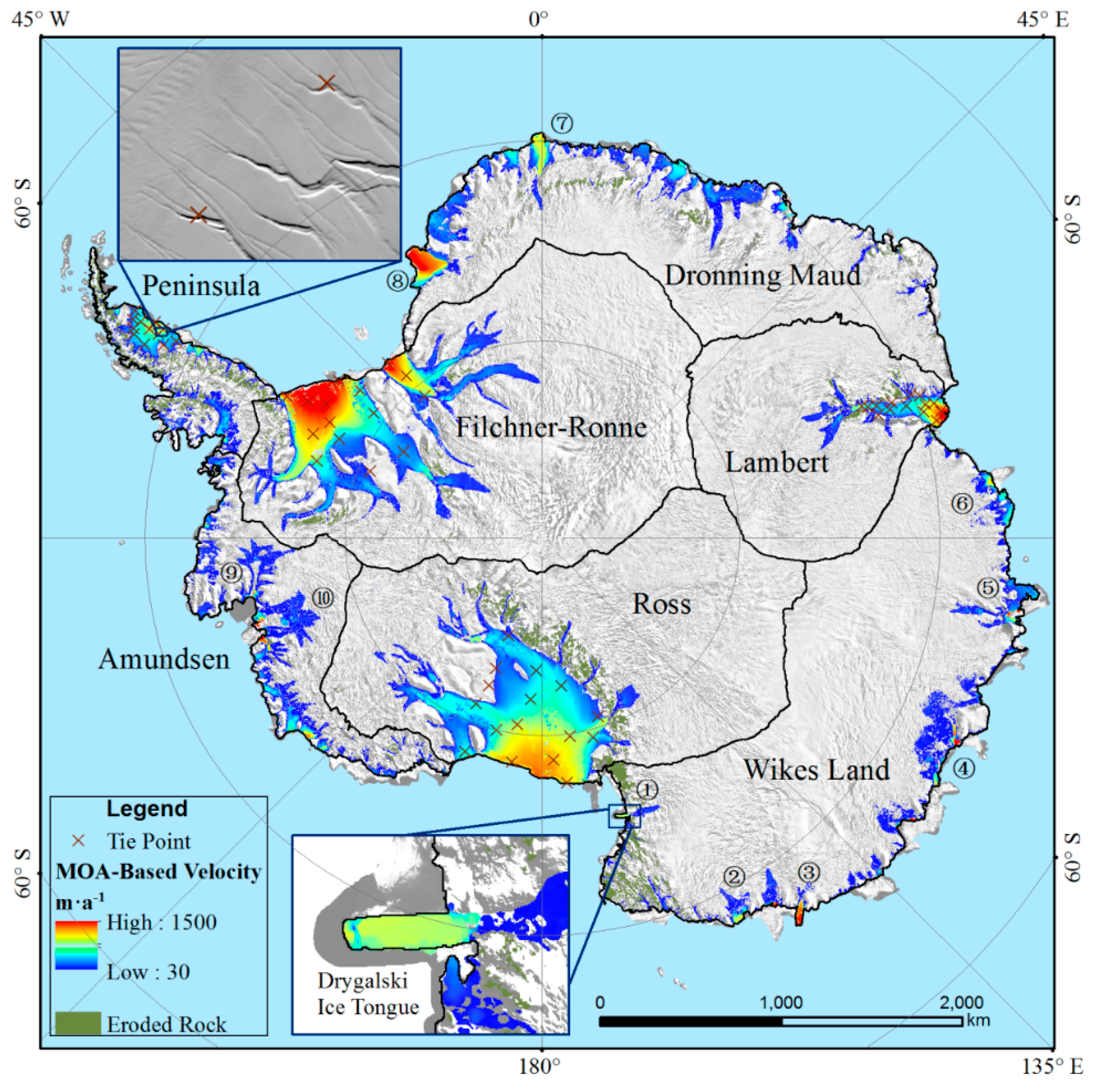
3.2. Antarctic and Greenland Ice
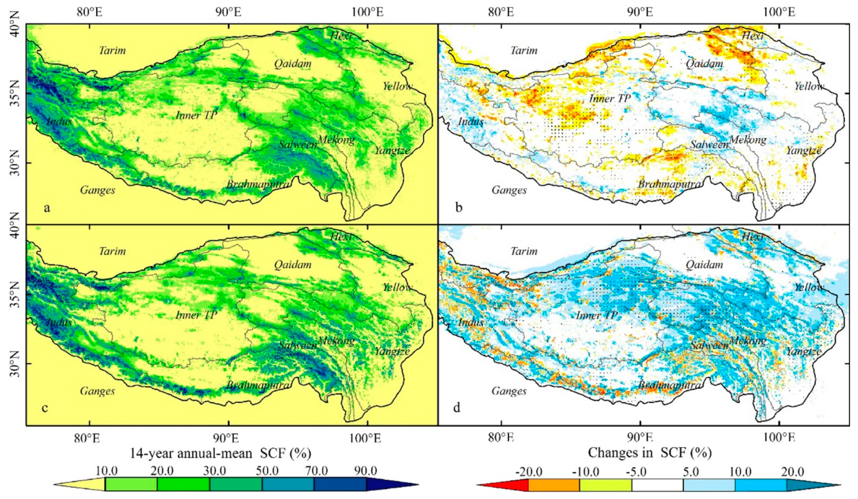
3.3. Tibetan Plateau
4. Challenges and Opportunities
4.1. Limitations of Current Approaches
4.2. Opportunities
5. Conclusions
Supplementary Materials
Author Contributions
Funding
Conflicts of Interest
Acronym list
| AGB | Aboveground biomass |
| APAR | Absorbed PAR |
| AMSR2 | Advanced Microwave Scanning Radiometer 2 |
| AMSR-E | Advanced Microwave Scanning Radiometer for Earth Observing System |
| ASAR | Advanced SAR |
| ATLAS | Advanced Topographic Laser Altimeter System |
| AVHRR | Advanced very-high-resolution radiometer |
| AMSR-E/2 | AMSR-E and AMSR2 |
| Tb | Brightness temperature |
| China–Brazil Earth Resources Satellite | CBERS-1 |
| DEM | Digital Elevation Model |
| DInSAR | Differential Interferometric Synthetic Aperture Radar |
| DMSP | Defense Meteorological Satellite Program |
| ERS | European remote sensing satellite |
| ETM | Enhanced Thematic Mapper |
| EVI | Enhanced Vegetation Index |
| FT | Freeze–thaw |
| FY | Feng Yun |
| GLAS | Geoscience Laser Altimeter System |
| GIMMS | Global Inventory Monitoring and Modeling System |
| GCOS | Global Climate Observing System |
| GNSS | Global Navigation Satellite System |
| GOES | Geostationary Operational Environmental Satellite |
| GRACE | Gravity Recovery and Climate Experiment |
| GBL | Great Bear Lake |
| GSL | Great Slave Lake |
| GPP | Gross Primary Productivity |
| ICESat | Ice, Cloud, and land Elevation Satellite |
| IMS | Interactive Multisensor Snow and Ice Mapping System |
| InSAR | Interferometric Synthetic Aperture Radar |
| ISRO | Indian Space Research Organisation |
| HKHT | Kush-Himalaya-Tibetan |
| LST | Land Surface Temperature |
| LAI | Leaf Area Index |
| LIDAR | Light Detection and Ranging |
| LUE | Light Use Efficiency |
| MBE | Mean Bias Error |
| MSG | Meteosat Second Generation |
| MWRI | Microwave Radiation Imager |
| MODIS | Moderate Resolution Imaging Spectroradiometer |
| MTSAT | Multifunctional Transport Satellites |
| NASA | National Aeronautics and Space Administration |
| NISAR | NASA-ISRO Synthetic Aperture Radar |
| NOAA | National Oceanic and Atmospheric Administration |
| NDSI | Normalized Difference Snow Index |
| NDVI | Normalized Difference Vegetation Index |
| NDFSI | Normalized Difference Forest Snow Index |
| Optical-IR | Optical and Infrared |
| OLI | Operational Land Imager |
| PSI | Persistent Scattered Interferometry |
| PALSAR | Phased Array type L-band Synthetic Aperture Radar |
| PAR | Photosynthetically active radiation |
| RMSE | Root Mean Square Error |
| SIRAL | SAR Interferometer Radar Altimeter |
| SMMR | Scanning Multichannel Microwave Radiometer |
| SWE | Snow water equivalent |
| SMAP | Soil Moisture Active Passive |
| SMOS | Soil Moisture and Ocean Salinity |
| SIF | Solar Induced Fluorescence |
| SSM/I | Special Sensor Microwave/Imager |
| SSMIS | Special Sensor Microwave Imager Sounder |
| SW | Surface water |
| SWOT | Surface Water Ocean Topography |
| SAR | Synthetic Aperture Radar |
| fPAR | The fraction of absorbed PAR |
| TM | Thematic Mapper |
| TP | Tibetan Plateau |
| TPSCE | Tibetan Plateau Snow Cover Extent record |
| UAV | Unmanned aerial vehicle |
| USGS | United States Geological Survey |
| VOD | Vegetation Optical Depth |
References
- Cohen, J.; Screen, J.A.; Furtado, J.C.; Barlow, M.; Whittleston, D.; Coumou, D.; Francis, J.; Dethloff, K.; Entekhabi, D.; Overland, J.; et al. Recent Arctic amplification and extreme mid-latitude weather. Nat. Geosci. 2014, 7, 627. [Google Scholar] [CrossRef]
- Stuecker, M.F.; Bitz, C.M.; Armour, K.C.; Proistosescu, C.; Kang, S.M.; Xie, S.P.; Kim, D.; McGregor, S.; Zhang, W.; Zhao, S.; et al. Polar amplification dominated by local forcing and feedbacks. Nat. Clim. Chang. 2018, 8, 1076. [Google Scholar] [CrossRef]
- Wang, B.; Bao, Q.; Hoskins, B.; Wu, G.X.; Liu, Y.M. Tibetan plateau warming and precipitation changes in East Asia. Geophys. Res. Lett. 2008, 35. [Google Scholar] [CrossRef]
- Xu, B.Q.; Cao, J.J.; Hansen, J.; Yao, T.D.; Joswia, D.R.; Wang, N.L.; Wu, G.J.; Wang, M.; Zhao, H.B.; Yang, W.; et al. Black soot and the survival of Tibetan glaciers. Proc. Natl. Acad. Sci. USA 2009, 106, 22114–22118. [Google Scholar] [CrossRef]
- Hugelius, G.; Routh, J.; Kuhry, P.; Crill, P. Mapping the degree of decomposition and thaw remobilization potential of soil organic matter in discontinuous permafrost terrain. J. Geophys. Res. Biogeosci. 2012, 117. [Google Scholar] [CrossRef]
- Olefeldt, D.; Goswami, S.; Grosse, G.; Hayes, D.; Hugelius, G.; Kuhry, P.; McGuire, A.D.; Romanovsky, V.E.; Sannel, A.B.K.; Schuur, E.A.G.; et al. Circumpolar distribution and carbon storage of thermokarst landscapes. Nat. Commun. 2016, 7, 13043. [Google Scholar] [CrossRef]
- Vaughan, D.G.; Marshall, G.J.; Connolley, W.M.; Parkinson, C.; Mulvaney, R.; Hodgson, D.A.; King, J.C.; Pudsey, C.J.; Turner, J. Recent rapid regional climate warming on the Antarctic Peninsula. Clim. Chang. 2003, 60, 243–274. [Google Scholar] [CrossRef]
- Huang, J.; Zhang, X.; Zhang, Q.; Lin, Y.; Hao, M.; Luo, Y.; Zhao, Z.; Yao, Y.; Chen, X.; Wang, L.; et al. Recently amplified arctic warming has contributed to a continual global warming trend. Nat. Clim. Chang. 2017, 7, 875. [Google Scholar] [CrossRef]
- Kim, Y.; Kimball, J.S.; Zhang, K.; Didan, K.; Velicogna, I.; McDonald, K.C. Attribution of divergent northern vegetation growth responses to lengthening non-frozen seasons using satellite optical-NIR and microwave Remote Sens. Int. J. Remote Sens. 2014, 35, 3700–3721. [Google Scholar] [CrossRef]
- Kim, Y.; Kimball, J.S.; Robinson, D.A.; Derksen, C. New satellite climate data records indicate strong coupling between recent frozen season changes and snow cover over high northern latitudes. Environ. Res. Lett. 2015, 10, 084004. [Google Scholar] [CrossRef]
- Schuur, E.A.; McGuire, A.D.; Schädel, C.; Grosse, G.; Harden, J.W.; Hayes, D.J.; Hugelius, G.; Koven, C.D.; Kuhry, P.; Lawrence, D.M.; et al. Climate change and the permafrost carbon feedback. Nature 2015, 520, 171. [Google Scholar] [CrossRef]
- Van Huissteden, J.; Dolman, A.J. Soil carbon in the Arctic and the permafrost carbon feedback. Curr. Opin. Environ. Sustain. 2012, 4, 545–551. [Google Scholar] [CrossRef]
- Pepin, N.; Bradley, R.S.; Diaz, H.F.; Baraër, M.; Caceres, E.B.; Forsythe, N.; Fowler, H.; Greenwood, G.; Hashmi, M.Z.; Liu, X.D.; et al. Elevation-dependent warming in mountain regions of the world. Nat. Clim. Chang. 2015, 5, 424. [Google Scholar]
- Zhu, Z.; Piao, S.; Myneni, R.B.; Huang, M.; Zeng, Z.; Canadell, J.G.; Ciais, P.; Sitch, S.; Friedlingstein, P.; Arneth, A.; et al. Greening of the Earth and its drivers. Nat. Clim. Chang. 2016, 6, 791–795. [Google Scholar] [CrossRef]
- Schuur, E.A.; Mack, M.C. Ecological response to permafrost thaw and consequences for local and global ecosystem services. Annu. Rev. Ecol. Evol. Syst. 2018, 49, 279–301. [Google Scholar] [CrossRef]
- Bormann, K.J.; Ross, D.B.; Chris, D.; Thomas, H. Painter. Estimating snow-cover trends from space. Nat. Clim. Chang. 2018, 8, 924–928. [Google Scholar] [CrossRef]
- Du, J.; Kimball, J.S.; Duguay, C.R.; Kim, Y.; Watts, J. Satellite microwave assessment of Northern Hemisphere lake ice phenology from 2002 to 2015. Cryosphere 2017, 11, 47–63. [Google Scholar] [CrossRef]
- Serreze, M.C.; Stroeve, J. Arctic sea ice trends, variability and implications for seasonal ice forecasting. Philos. Trans. R. Soc. A Math. Phys. Eng. Sci. 2015, 373, 20140159. [Google Scholar] [CrossRef]
- Rignot, E.; Mouginot, J.; Scheuchl, B.; van den Broeke, M.; van Wessem, M.J.; Morlighem, M. Four decades of Antarctic Ice Sheet mass balance from 1979–2017. Proc. Natl. Acad. Sci. USA 2019, 116, 1095–1103. [Google Scholar] [CrossRef]
- Flanner, M.G.; Shell, K.M.; Barlage, M.; Perovich, D.K.; Tschudi, M.A. Radiative forcing and albedo feedback from the Northern Hemisphere cryosphere between 1979 and 2008. Nat. Geosci. 2011, 4, 151. [Google Scholar] [CrossRef]
- Kim, Y.; Kimball, J.S.; Du, J.; Schaaf, C.L.B.; Kirchner, P.B. Quantifying the effects of freeze-thaw transitions and snowpack melt on land surface albedo and energy exchange over Alaska and Western Canada. Environ. Res. Lett. 2018, 13, 075009. [Google Scholar] [CrossRef]
- Duan, L.; Cao, L.; Caldeira, K. Estimating Contributions of Sea Ice and Land Snow to Climate Feedback. J. Geophys. Res. Atmos. 2019, 124, 199–208. [Google Scholar] [CrossRef]
- Boelman, N.T.; Liston, G.E.; Gurarie, E.; Meddens, A.J.; Mahoney, P.J.; Kirchner, P.B.; Bohrer, G.; Brinkman, T.J.; Cosgrove, C.L.; Eitel, J.U.; et al. Integrating snow science and wildlife ecology in Arctic-boreal North America. Environ. Res. Lett. 2019, 14, 010401. [Google Scholar] [CrossRef]
- Liljedahl, A.K.; Boike, J.; Daanen, R.P.; Fedorov, A.N.; Frost, G.V.; Grosse, G.; Hinzman, L.D.; Iijma, Y.; Jorgenson, J.C.; Matveyeva, N.; et al. Pan-Arctic ice-wedge degradation in warming permafrost and its influence on tundra hydrology. Nat. Geosci. 2016, 9, 312. [Google Scholar] [CrossRef]
- Turetsky, M.R.; Abbott, B.W.; Jones, M.C.; Anthony, K.W.; Olefeldt, D.; Schuur, E.A.; Koven, C.; McGuire, A.D.; Grosse, G.; Kuhry, P.; et al. Permafrost collapse is accelerating carbon release. Nature 2019, 569, 32–34. [Google Scholar] [CrossRef] [PubMed]
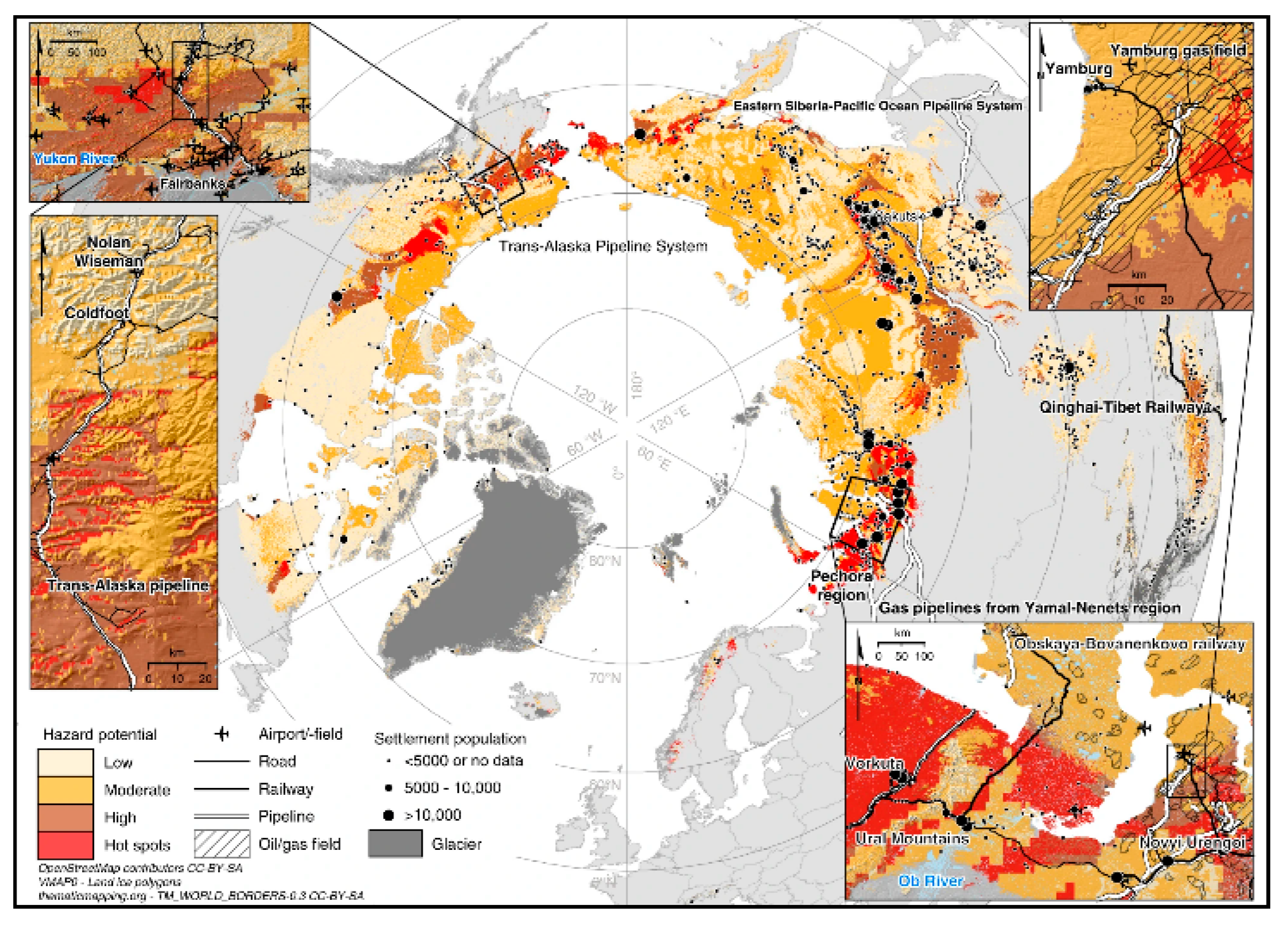
- Hjort, J.; Karjalainen, O.; Aalto, J.; Westermann, S.; Romanovsky, V.E.; Nelson, F.E.; Etzelmüller, B.; Luoto, M. Degrading permafrost puts Arctic infrastructure at risk by mid-century. Nat. Commun. 2018, 9, 5147. [Google Scholar] [CrossRef] [PubMed]
- Walvoord, M.A.; Kurylyk, B.L. Hydrologic impacts of thawing permafrost—A review. Vadose Zone J. 2016, 15. [Google Scholar] [CrossRef]
- Smith, L.C.; Sheng, Y.; MacDonald, G.M.; Hinzman, L.D. Disappearing arctic lakes. Science 2005, 308, 1429. [Google Scholar] [CrossRef]
- Watts, J.D.; Kimball, J.S.; Jones, L.A.; Schroeder, R.; McDonald, K.C. Satellite Microwave remote sensing of contrasting surface water inundation changes within the Arctic–Boreal Region. Remote Sens. Environ. 2012, 127, 223–236. [Google Scholar] [CrossRef]
- Andresen, C.G.; Lougheed, V.L. Disappearing Arctic tundra ponds: Fine-scale analysis of surface hydrology in drained thaw lake basins over a 65 year period (1948–2013). J. Geophys. Res. Biogeosci. 2015, 120, 466–479. [Google Scholar] [CrossRef]
- Park, T.; Ganguly, S.; Tømmervik, H.; Euskirchen, E.S.; Høgda, K.-A.; Karlsen, S.R.; Brovkin, V.; Nemani, R.R.; Myneni, R.B. Changes in growing season duration and productivity of northern vegetation inferred from long-term remote sensing data. Environ. Res. Lett. 2016, 11. [Google Scholar] [CrossRef]
- Soja, A.J.; Tchebakova, N.M.; French, N.H.; Flannigan, M.D.; Shugart, H.H.; Stocks, B.J.; Sukhinin, A.I.; Parfenova, E.I.; Chapin, F.S., III; Stackhouse, P.W., Jr. Climate-induced boreal forest change: Predictions versus current observations. Glob. Planet. Chang. 2007, 56, 274–296. [Google Scholar] [CrossRef]
- Loranty, M.M.; Lieberman-Cribbin, W.; Berner, L.T.; Natali, S.M.; Goetz, S.J.; Alexander, H.D.; Kholodov, A.L. Spatial variation in vegetation productivity trends, fire disturbance, and soil carbon across arctic-boreal permafrost ecosystems. Environ. Res. Lett. 2016, 11, 095008. [Google Scholar] [CrossRef]
- Park, H.; Kim, Y.; Kimball, J.S. Widespread permafrost vulnerability and soil active layer increases over the high northern latitudes inferred from satellite remote sensing and process model assessments. Remote Sens. Environ. 2016, 175, 349–358. [Google Scholar] [CrossRef]
- Kim, Y.; Kimball, J.S.; Glassy, J.; Du, J. An extended global earth system data record on daily landscape freeze-thaw status determined from satellite passive microwave Remote Sens. Earth Syst. Sci. Data 2017, 9, 133–147. [Google Scholar] [CrossRef]
- Potter, C. Recovery Rates of Wetland Vegetation Greenness in Severely Burned Ecosystems of Alaska Derived from Satellite Image Analysis. Remote Sens. 2018, 10, 1456. [Google Scholar] [CrossRef]
- Pan, C.G.; Kirchner, P.B.; Kimball, J.S.; Kim, Y.; Du, J. Rain-on-snow events in Alaska, their frequency and distribution from satellite observations. Environ. Res. Lett. 2018, 13, 075004. [Google Scholar] [CrossRef]
- Du, J.; Kimball, J.S.; Azarderakhsh, M.; Dunbar, R.S.; Moghaddam, M.; McDonald, K.C. Classification of Alaska spring thaw characteristics using satellite L-band radar Remote Sens. IEEE Trans. Geosci. Remote Sens. 2014, 53, 542–556. [Google Scholar]
- Montgomery, J.; Brisco, B.; Chasmer, L.; Devito, K.; Cobbaert, D.; Hopkinson, C. SAR and Lidar Temporal Data Fusion Approaches to Boreal Wetland Ecosystem Monitoring. Remote Sens. 2019, 11, 161. [Google Scholar] [CrossRef]
- Davidson, S.; Santos, M.; Sloan, V.; Watts, J.; Phoenix, G.; Oechel, W.; Zona, D. Mapping Arctic tundra vegetation communities using field spectroscopy and multispectral satellite data in North Alaska, USA. Remote Sens. 2016, 8, 978. [Google Scholar] [CrossRef]
- Lindenschmidt, K.E.; Li, Z. Radar Scatter Decomposition to Differentiate between Running Ice Accumulations and Intact Ice Covers along Rivers. Remote Sens. 2019, 11, 307. [Google Scholar] [CrossRef]
- Veh, G.; Korup, O.; Roessner, S.; Walz, A. Detecting Himalayan glacial lake outburst floods from Landsat time series. Remote Sens. Environ. 2018, 207, 84–97. [Google Scholar] [CrossRef]
- Rondeau-Genesse, G.; Trudel, M.; Leconte, R. Monitoring snow wetness in an Alpine Basin using combined C-band SAR and MODIS data. Remote Sens. Environ. 2016, 183, 304–317. [Google Scholar] [CrossRef]
- Shi, J.; Dozier, J. Estimatino of snow water equivalence using SIR-C/X-SAR, Part I: Inferring snow density and subsurface properties. IEEE Trans. Geosci. Remote Sens. 2000, 38, 2465–2474. [Google Scholar]
- Shi, J.; Dozier, J. Estimation of snow water equivalence using SIR-C/X-SAR, Part II: Inferring snow depth and particle size. IEEE Trans. Geosci. Remote Sens. 2000, 38, 2475–2488. [Google Scholar]
- Rautiainen, K.; Parkkinen, T.; Lemmetyinen, J.; Schwank, M.; Wiesmann, A.; Ikonen, J.; Derksen, C.; Davydov, S.; Davydova, A.; Boike, J.; et al. SMOS prototype algorithm for detecting autumn soil freezing. Remote Sens. Environ. 2016, 180, 346–360. [Google Scholar] [CrossRef]
- Baghdadi, N.; Bazzi, H.; El Hajj, M.; Zribi, M. Detection of frozen soil using Sentinel-1 SAR data. Remote Sens. 2018, 10, 1182. [Google Scholar] [CrossRef]
- Chen, X.; Liu, L.; Bartsch, A. Detecting soil freeze/thaw onsets in Alaska using SMAP and ASCAT data. Remote Sens. Environ. 2019, 220, 59–70. [Google Scholar] [CrossRef]
- Jansson, P.; Hock, R.; Schneider, T. The concept of glacier storage: A review. J. Hydrol. 2003, 282, 116–129. [Google Scholar] [CrossRef]
- Williams, R.S. Glaciers: Clues to Future Climate? United States Geological Survey: Denver, CO, USA, 1983.
- Sasgen, I.; Konrad, H.; Helm, V.; Grosfeld, K. High-Resolution Mass Trends of the Antarctic Ice Sheet through a Spectral Combination of Satellite Gravimetry and Radar Altimetry Observations. Remote Sens. 2019, 11, 144. [Google Scholar] [CrossRef]
- Wahr, J.; Swenson, S.; Zlotnicki, V.; Velicogna, I. Time-variable gravity from GRACE: First results. Geophys. Res. Lett. 2004, 31. [Google Scholar] [CrossRef]
- Wesche, C.; Jansen, D.; Dierking, W. Calving fronts of Antarctica: Mapping and classification. Remote Sens. 2013, 5, 6305–6322. [Google Scholar] [CrossRef]
- Wang, X.; Cheng, X.; Gong, P.; Huang, H.; Li, Z.; Li, X. Earth science applications of ICESat/GLAS: A review. Int. J. Remote Sens. 2011, 32, 8837–8864. [Google Scholar] [CrossRef]
- Markus, T.; Neumann, T.; Martino, A.; Abdalati, W.; Brunt, K.; Csatho, B.; Farrell, S.; Fricker, H.; Gardner, A.; Harding, D.; et al. The Ice, Cloud, and land Elevation Satellite-2 (ICESat-2): Science requirements, concept, and implementation. Remote Sens. Environ. 2017, 190, 260–273. [Google Scholar] [CrossRef]
- Cook, A.J.; Murray, T.; Luckman, A.; Vaughan, D.G.; Barrand, N.E. A new 100-m Digital Elevation Model of the Antarctic Peninsula derived from ASTER Global DEM: Methods and accuracy assessment. Earth Syst. Sci. Data 2012, 4, 129–142. [Google Scholar] [CrossRef]
- Toutin, T.; Schmitt, C.; Berthier, E.; Clavet, D. DEM generation over ice fields in the Canadian Arctic with along-track SPOT5 HRS stereo data. Can. J. Remote Sens. 2012, 37, 429–438. [Google Scholar] [CrossRef]
- McMillan, M.; Shepherd, A.; Sundal, A.; Briggs, K.; Muir, A.; Ridout, A.; Hogg, A.; Wingham, D. Increased ice losses from Antarctica detected by CryoSat-2. Geophys. Res. Lett. 2014, 41, 3899–3905. [Google Scholar] [CrossRef]
- Fahnestock, M.; Scambos, T.; Moon, T.; Gardner, A.; Haran, T.; Klinger, M. Rapid large-area mapping of ice flow using Landsat 8. Remote Sens. Environ. 2016, 185, 84–94. [Google Scholar] [CrossRef]
- Li, T.; Liu, Y.; Li, T.; Hui, F.; Chen, Z.; Cheng, X. Antarctic Surface Ice Velocity Retrieval from MODIS-Based Mosaic of Antarctica (MOA). Remote Sens. 2018, 10, 1045. [Google Scholar] [CrossRef]
- Strozzi, T.; Luckman, A.; Murray, T.; Wegmuller, U.; Werner, C.L. Glacier motion estimation using SAR offset-tracking procedures. IEEE Trans. Geosci. Remote Sens. 2002, 40, 2384–2391. [Google Scholar] [CrossRef]
- Cheng, X.; Xu, G. The integration of JERS-1 and ERS SAR in differential interferometry for measurement of complex glacier motion. J. Glaciol. 2006, 52, 80–88. [Google Scholar] [CrossRef]
- Gourmelen, N.; Kim, S.W.; Shepherd, A.; Park, J.W.; Sundal, A.V.; Björnsson, H.; Pálsson, F. Ice velocity determined using conventional and multiple-aperture InSAR. Earth Planet. Sci. Lett. 2011, 307, 156–160. [Google Scholar] [CrossRef]
- Brown, L.C.; Duguay, C.R. The response and role of ice cover in lake-climate interactions. Prog. Phys. Geogr. 2010, 34, 671–704. [Google Scholar] [CrossRef]
- Eerola, K.L.; Rontu, E.; Kourzeneva, H.; Kheyrollah, P.; Duguay, C.R. Impact of partly ice-free Lake Ladoga on temperature and cloudiness in an anticyclonic winter situation—A case study using HIRLAM model. Tellus Ser. A Dyn. Meteorol. Oceanogr. 2014, 66, 23929. [Google Scholar] [CrossRef]
- Baijnath-Rodino, J.A.; Duguay, C.R. Historical spatiotemporal trends in snowfall extremes over the Canadian domain of the Great Lakes Basin. Adv. Meteorol. 2018, 2018. [Google Scholar] [CrossRef]
- Baijnath-Rodino, J.A.; Duguay, C.R.; LeDrew, E.F. Climatological trends of snowfall over the Laurentian Great Lakes Basin. Int. J. Climatol. 2018, 38, 3942–3962. [Google Scholar] [CrossRef]
- Baijnath-Rodino, J.A.; Duguay, C.R. Assessment of coupled CRCM5-FLake on the reproduction of wintertime lake-induced precipitation in the Great Lakes Basin. Theor. Appl. Climatol. 2019. [Google Scholar] [CrossRef]
- GCOS. The Global Observing System for Climate: Implementation Needs, GCOS-200; GCOS 2016 Implementation Plan; World Meteorological Organization: Geneva, Switzerland, 2016; p. 315. [Google Scholar]
- Duguay, C.R.; Prowse, T.D.; Bonsal, B.R.; Brown, R.D.; Lacroix, M.P.; Ménard, P. Recent trends in Canadian lake ice cover. Hydrol. Process. 2006, 20, 781–801. [Google Scholar] [CrossRef]
- Derksen, C.; Burgess, D.; Duguay, C.; Howell, S.; Mudryk, L.; Smith, S.; Thackeray, C.; Kirchmeier-Young, M. Changes in Snow, Ice, and Permafrost across CANADA; Chapter 5 in Canada’s Changing Climate, Report; Bush, E., Lemmen, D.S., Eds.; Government of Canada: Ottawa, ON, USA, 2019; pp. 194–260.
- Surdu, C.M.; Duguay, C.R.; Fernández Prieto, D. Evidence of recent changes in the ice regime of high arctic lakes from spaceborne satellite observations. Cryosphere 2016, 10, 941–960. [Google Scholar] [CrossRef]
- Engram, M.; Arp, C.D.; Jones, B.M.; Ajadi, O.A.; Meyer, F.J. Analyzing floating and bedfast lake ice regimes across Arctic Alaska using 25 years of space-borne SAR imagery. Remote Sens. Environ. 2018, 209, 660–676. [Google Scholar] [CrossRef]
- Duguay, C.; Brown, L. 2018: Lake Ice [in Arctic Report Card 2018. Available online: https://www.arctic.noaa.gov/Report-Card (accessed on 15 May 2019).
- National Ice Center. IMS Daily Northern Hemisphere Snow and Ice Analysis at 1 km, 4 km, and 24 km Resolutions, Version 1; NASA National Snow and Ice Data Center Distributed Active Archive Center: Boulder, CO, USA, 2008; updated daily. [CrossRef]
- Duguay, C.; Brown, L.; Kang, K.-K.; Pour, H.K. The Arctic Lake ice In State of the Climate in 2014. Bull. Am. Meteorol. Soc. 2015, 96, S144–S145. [Google Scholar]
- Cai, Y.; Ke, C.Q.; Li, X.; Zhang, G.; Duan, Z.; Lee, H. Variations of lake ice phenology on the Tibetan Plateau From 2001 to 2017 based on MODIS Data. J. Geophys. Res. Atmos. 2019, 124, 1–19. [Google Scholar] [CrossRef]
- Chen, J.; Wang, Y.; Cao, L.; Zheng, J. Variations in the ice phenology and water level of Ayakekumu Lake, Tibetan Plateau, derived from MODIS and satellite altimetry data. J. Indian Soc. Remote Sens. 2018, 46, 1689–1699. [Google Scholar] [CrossRef]
- Gou, P.; Ye, Q.; Che, T.; Feng, Q.; Ding, B.; Lin, C.; Zong, J. Lake ice phenology of Nam Co, Central Tibetan Plateau, China, derived from multiple MODIS data products. J. Great Lakes Res. 2017, 43, 989–998. [Google Scholar] [CrossRef]
- Murfitt, J.; Brown, L.C. Lake ice and temperature trends for Ontario and Manitoba: 2001 to 2014. Hydrol. Process. 2017, 31, 3596–3609. [Google Scholar] [CrossRef]
- Qi, M.; Yao, X.; Li, X.; Duan, H.; Gao, Y.; Liu, J. Spatiotemporal characteristics of Qinghai Lake ice phenology between 2000 and 2016. J. Geogr. Sci. 2019, 29, 115–130. [Google Scholar] [CrossRef]
- Šmejkalová, T.; Edwards, M.E.; Dash, J. Arctic lakes show strong decadal trend in earlier spring ice-out. Sci. Rep. 2016, 6, 1–8. [Google Scholar] [CrossRef]
- Kang, K.-K.; Duguay, C.R.; Howell, S.E.L. Estimating ice phenology on large northern lakes from AMSR-E: Algorithm development and application to Great Bear Lake and Great Slave Lake, Canada. Cryosphere 2012, 6, 235–254. [Google Scholar] [CrossRef]
- Kang, K.-K.; Duguay, C.R.; Lemmetyinen, J.; Gel, Y. Estimation of ice thickness on large northern lakes from AMSR-E brightness temperature measurements. Remote Sens. Environ. 2014, 150, 1–19. [Google Scholar] [CrossRef]
- Wang, J.; Duguay, C.R.; Clausi, D.A.; Pinard, V.; Howell, S.E.L. Semi-automated classification of lake ice cover using dual polarization RADARSAT-2 imagery. Remote Sens. 2018, 10, 1727. [Google Scholar] [CrossRef]
- Leigh, S.; Wang, Z.; Clausi, D.A. Automated ice-water classification using dual polarization SAR satellite imagery. IEEE Trans. Geosci. Remote Sens. 2014, 52, 5529–5539. [Google Scholar] [CrossRef]
- Murfitt, J.; Brown, L.C.; Howell, S.E.L. Evaluating RADARSAT-2 for the automated monitoring of lake Ice phenology events in mid-latitudes. Remote Sens. 2018, 10, 1641. [Google Scholar] [CrossRef]
- Surdu, C.M.; Duguay, C.R.; Pour, H.K.; Brown, L.C. Ice freeze-up and break-up detection of shallow lakes in Northern Alaska with spaceborne SAR. Remote Sens. 2015, 7, 6133–6159. [Google Scholar] [CrossRef]
- Beckers., J.F.; Casey, J.A.; Haas, C. Retrievals of lake ice thickness from Great Slave Lake and Great Bear Lake using CryoSat-2. IEEE Trans. Geosci. Remote Sens. 2017, 55, 3708–3720. [Google Scholar] [CrossRef]
- Murfitt, J.C.; Brown, L.C.; Howell, S.E.L. Estimating lake ice thickness in Central Ontario. PLoS ONE 2018, 13, e0208519. [Google Scholar] [CrossRef] [PubMed]
- Pour, H.K.; Duguay, C.R.; Scott, A.; Kang, K.-K. Improvement of lake ice thickness retrieval from MODIS satellite data using a thermodynamic model. IEEE Trans. Geosci. Remote Sens. 2017, 55, 5956–5965. [Google Scholar] [CrossRef]
- Duguay, C.R.; Flato, G.M.; Jeffries, M.O.; Ménard, P.; Morris, K.; Rouse, W.R. Ice cover variability on shallow lakes at high latitudes: Model simulations and observations. Hydrol. Process. 2003, 17, 3465–3483. [Google Scholar] [CrossRef]
- Duguay, C.R.; Bernier, M.; Gauthier, Y.; Kouraev, A. Remote sensing of lake and river ice. In Remote Sensing of the Cryosphere; Tedesco, M., Ed.; Wiley-Blackwell: Oxford, UK, 2015; pp. 273–306. [Google Scholar]
- Atwood, D.; Gunn, G.; Roussi, C.; Wu, J.; Duguay, C.; Sarabandi, K. Microwave backscatter from Arctic lake ice and polarimetric implications. IEEE Trans. Geosci. Remote Sens. 2015, 53, 5972–5982. [Google Scholar] [CrossRef]
- Gunn, G.; Duguay, C.; Atwood, D.; King, J.; Toose, P. Observing scattering mechanisms of bubbled freshwater lake ice using polarimetric RADARSAT-2 (C-band) and UWScat (X-, Ku-band). IEEE Trans. Geosci. Remote Sens. 2018, 56, 2887–2903. [Google Scholar] [CrossRef]
- Surdu, C.M.; Duguay, C.R.; Brown, L.C.; Fernández Prieto, D. Response of ice cover on shallow lakes of the North Slope of Alaska to contemporary climate conditions (1950–2011): Radar remote-sensing and numerical modeling data analysis. Cryosphere 2014, 8, 167–180. [Google Scholar] [CrossRef]
- Antonova, S.; Duguay, C.; Kääb, A.; Heim, B.; Langer, M.; Westermann, S.; Boike, J. Monitoring bedfast ice and ice phenology in lakes of the Lena river delta using TerraSAR-X backscatter and coherence time series. Remote Sens. 2016, 8, 903. [Google Scholar] [CrossRef]
- Barnett, T.P.; Adam, J.C.; Lettenmaier, D.P. Potential impacts of a warming climate on water availability in snow-dominated regions. Nature 2005, 438, 303–309. [Google Scholar] [CrossRef] [PubMed]
- Tsai, Y.L.S.; Dietz, A.; Oppelt, N.; Kuenzer, C. Remote Sensing of Snow Cover Using Spaceborne SAR: A Review. Remote Sens. 2019, 11, 1456. [Google Scholar] [CrossRef]
- Dozier, J. Spectral signature of alpine snow cover from the Landsat Thematic Mapper. Remote Sens. Environ. 1989, 28, 9–22. [Google Scholar] [CrossRef]
- Hüsler, F.; Jonas, T.; Wunderle, S.; Albrecht, S. Validation of a modified snow cover retrieval algorithm from historical 1-km AVHRR data over the European Alps. Remote Sens. Environ. 2012, 121, 497–515. [Google Scholar] [CrossRef]
- Hall, D.K.; Riggs, G.A.; Salomonson, V.V.; DiGirolamo, N.E.; Bayr, K.J. MODIS snow-cover products. Remote Sens. Environ. 2002, 83, 181–194. [Google Scholar] [CrossRef]
- Wang, X.; Wang, J.; Che, T.; Huang, X.; Hao, X.; Li, H. Snow cover mapping for complex mountainous forested environments based on a multi-index technique. IEEE J. Sel. Top. Appl. Earth Obs. Remote Sens. 2018, 11, 1433–1441. [Google Scholar] [CrossRef]
- Metsämäki, S.; Mattila, O.-P.; Pulliainen, J.; Niemi, K.; Luojus, K.; Böttcher, K. An optical reflectance model-based method for fractional snow cover mapping applicable to continental scale. Remote Sens. Environ. 2012, 123, 508–521. [Google Scholar] [CrossRef]
- Hori, M.; Sugiura, K.; Kobayashi, K.; Aoki, T.; Tanikawa, T.; Kuchiki, K.; Niwano, M.; Enomoto, H. A 38-year (1978–2015) Northern Hemisphere daily snow cover extent product derived using consistent objective criteria from satellite-borne optical sensors. Remote Sens. Environ. 2017, 191, 402–418. [Google Scholar] [CrossRef]
- Wayand, N.E.; Marsh, C.B.; Shea, J.M.; Pomeroy, J.W. Globally scalable alpine snow metrics. Remote Sens. Environ. 2018, 213, 61–72. [Google Scholar] [CrossRef]
- Gascoin, S.; Grizonnet, M.; Bouchet, M.; Salgues, G.; Hagolle, O. Theia Snow collection: High-resolution operational snow cover maps from Sentinel-2 and Landsat-8 data. Earth Syst. Sci. Data 2019, 11, 493–514. [Google Scholar] [CrossRef]
- Moosavi, V.; Malekinezhad, H.; Shirmohammadi, B. Fractional snow cover mapping from MODIS data using wavelet-artificial intelligence hybrid models. J. Hydrol. 2014, 511, 160–170. [Google Scholar] [CrossRef]
- Czyzowska-Wisniewski, E.H.; van Leeuwen, W.J.D.; Hirschboeck, K.K.; Marsh, S.E.; Wisniewski, W.T. Fractional snow cover estimation in complex alpine-forested environments using an artificial neural network. Remote Sens. Environ. 2015, 156, 403–417. [Google Scholar] [CrossRef]
- Roesch, A.; Wild, M.; Gilgen, H.; Ohmura, A.; Arugnell, N.C. A new snow cover fraction parameterization for the ECHAM4 GCM. Clim. Dyn. 2001, 17, 933–946. [Google Scholar] [CrossRef]
- Salomonson, V.V.; Appel, I. Estimating fractional snow cover from MODIS using the normalized difference snow index. Remote Sens. Environ. 2004, 89, 351–360. [Google Scholar] [CrossRef]
- Vikhamar, D.; Solberg, R. Snow-cover mapping in forests by constrained linear spectral unmixing of MODIS data. Remote Sens. Environ. 2003, 88, 309–323. [Google Scholar] [CrossRef]
- Mishra, V.D.; Negi, H.S.; Rawat, A.K.; Chaturvedi, A.; Singh, R.P. Retrieval of sub-pixel snow cover information in the Himalayan region using medium and coarse resolution remote sensing data. Int. J. Remote. Sens. 2009, 30, 4707–4731. [Google Scholar] [CrossRef]
- Painter, T.H.; Rittger, K.; McKenzie, C.; Slaughter, P.; Davis, R.E.; Dozier, J. Retrieval of subpixel snow covered area, grain size, and albedo from MODIS. Remote Sens. Environ. 2009, 113, 868–879. [Google Scholar] [CrossRef]
- Sirguey, P.; Mathieu, R.; Arnaud, Y. Subpixel monitoring of the seasonal snow cover with MODIS at 250 m spatial resolution in the Southern Alps of New Zealand: Methodology and accuracy assessment. Remote Sens. Environ. 2009, 113, 160–181. [Google Scholar] [CrossRef]
- Hao, S.; Jiang, L.; Shi, J.; Wang, G.; Liu, X. Assessment of MODIS-Based Fractional Snow Cover Products Over the Tibetan Plateau. IEEE J. Sel. Top. Appl. Earth Obs. Remote Sens. 2018, 12, 533–548. [Google Scholar] [CrossRef]
- Romanov, P.; Tarpley, D. Enhanced algorithm for estimating snow depth from geostationary satellites. Remote Sens. Environ. 2007, 108, 97–110. [Google Scholar] [CrossRef]
- De Ruyter de Wildt, M.; Seiz, G.; Gruen, A. Operational snow mapping using multitemporal Meteosat SEVIRI imagery. Remote Sens. Environ. 2007, 109, 29–41. [Google Scholar] [CrossRef]
- Siljamo, N.; Hyvärinen, O. New geostationary satellite-based snow-cover algorithm. J. Appl. Meteorol. Clim. 2011, 50, 1275–1290. [Google Scholar] [CrossRef]
- Yang, J.; Jiang, L.; Wu, F.; Sun, R. Monitoring snow cover over China with MTSAT-2 geostationary satellite. J. Remot. Sens. 2013, 17, 1264–1280. [Google Scholar]
- Yang, J.; Jiang, L.; Shi, J.; Wu, S.; Sun, R.; Yang, H. Monitoring snow cover using Chinese meteorological satellite data over China. Remote Sens. Environ. 2014, 143, 192–203. [Google Scholar] [CrossRef]
- Wang, G.; Jiang, L.; Wu, S.; Shi, J.; Hao, S.; Liu, X. Fractional Snow Cover Mapping from FY-2 VISSR Imagery of China. Remote Sens. 2017, 9, 983. [Google Scholar] [CrossRef]
- Gao, Y.; Xie, H.; Lu, N.; Yao, T.; Liang, T. Toward advanced daily cloud-free snow cover and snow water equivalent products from Terra–Aqua MODIS and Aqua AMSR-E measurements. J. Hydrol. 2010, 385, 23–35. [Google Scholar] [CrossRef]
- Liang, T.; Zhang, X.; Xie, H.; Wu, C.; Feng, Q.; Huang, X.; Chen, Q. Toward improved daily snow cover mapping with advanced combination of MODIS and AMSR-E measurements. Remote Sens. Environ. 2008, 112, 3750–3761. [Google Scholar] [CrossRef]
- Yang, J.; Jiang, L.; Wu, S.; Wang, G.; Wang, J.; Liu, X. Development of a Snow Depth Estimation Algorithm over China for the FY-3D/MWRI. Remote Sens. 2019, 11, 977. [Google Scholar] [CrossRef]
- Helfrich, S.R.; McNamara, D.; Ramsay, B.H.; Baldwin, T.; Kasheta, T. Enhancements to, and forthcoming developments in the Interactive Multisensor Snow and Ice Mapping System (IMS). Hydrol. Process. 2007, 21, 1576–1586. [Google Scholar] [CrossRef]
- Qiu, Y.; Guo, H.; Chu, D.; Zhang, H.; Shi, J.; Shi, L.; Zheng, Z. MODIS daily cloud-free snow cover products over Tibetan Plateau. Sci. Data Bank 2016. [Google Scholar] [CrossRef]
- Hoang, T.; Phu, N.; Mohammed, O.; Kuo-lin, H.; Soroosh, S.; Xia, Q. A cloud-free MODIS snow cover dataset for the contiguous United States from 2000 to 2017. Sci. Data 2019, 6, 180300. [Google Scholar]
- Du, J.; Shi, J.; Tjuatja, S.; Chen, K.S. A combined method to model microwave scattering from a forest medium. IEEE Trans. Geosci. Remote Sens. 2006, 44, 815–824. [Google Scholar]
- Jiang, L.; Wang, P.; Zhang, L.; Yang, H.; Yang, J. Improvement of snow depth retrieval for FY3B-MWRI in China. Sci. China Earth Sci. 2014, 57, 1278–1292. [Google Scholar] [CrossRef]
- Kelly, R. The AMSR-E Snow Depth Algorithm: Description and Initial Results. Remote Sens. Soc. Jpn. 2009, 29, 307–317. [Google Scholar]
- Tedesco, M.; Reichle, R.; Low, A.; Markus, T.; Foster, J.L. Dynamic approaches for snow depth retrieval from spaceborne microwave brightness temperature. IEEE Trans. Geosci. Remote Sens. 2010, 48, 1955–1967. [Google Scholar] [CrossRef]
- Pulliainen, J.; Hallikainen, M. Retrieval of regional snow water equivalent from space-borne passive microwave observations. Remote Sens. Environ. 2001, 75, 76–85. [Google Scholar] [CrossRef]
- Jiang, L.; Shi, J.; Tjuatja, S.; Chen, K.S.; Du, J.; Zhang, L. Estimation of snow water equivalence using the polarimetric scanning radiometer from the cold land processes experiments (CLPX03). IEEE Geosci. Remote Sens. Lett. 2011, 8, 359–363. [Google Scholar] [CrossRef]
- Pan, J.; Durand, M.T.; Vander Jagt, B.J.; Liu, D. Application of a Markov Chain Monte Carlo algorithm for snow water equivalent retrieval from passive microwave measurements. Remote Sens. Environ. 2017, 192, 150–165. [Google Scholar] [CrossRef]
- Santi, E.; Pettinato, S.; Paloscia, S.; Pampaloni, P.; Macelloni, G.; Brogioni, M. An algorithm for generating soil moisture and snow depth maps from microwave spaceborne radiometers: HydroAlgo. Hydrol. Earth Syst. Sci. 2012, 16, 3659–3676. [Google Scholar] [CrossRef]
- Bair, E.H.; Abreu Calfa, A.; Rittger, K.; Dozier, J. Using machine learning for real-time estimates of snow water equivalent in the watersheds of Afghanistan. Cryosphere 2018, 12, 1579–1594. [Google Scholar] [CrossRef]
- Che, T.; Li, X.; Jin, R.; Huang, C. Assimilating passive microwave remote sensing data into a land surface model to improve the estimation of snow depth. Remote Sens. Environ. 2014, 143, 54–63. [Google Scholar] [CrossRef]
- Larue, F.; Royer, A.; Sève, D.D.; Roy, A.; Cosme, E. Assimilation of passive microwave AMSR-2 satellite observations in a snowpack evolution model over northeastern Canada. Hydrol. Earth Syst. Sci. 2018, 22, 5711–5734. [Google Scholar] [CrossRef]
- Rott, H.; Yueh, S.H.; Cline, D.W.; Duguay, C.; Essery, R.; Haas, C.; Heliere, F.; Kern, M.; MacElloni, G.; Malnes, E.; et al. Cold regions hydrology high-resolution observatory for snow and cold land processes. Proc. IEEE 2010, 98, 752–765. [Google Scholar] [CrossRef]
- Du, J.; Shi, J.; Rott, H. Comparison between a multi-scattering and multi-layer snow scattering model and its parameterized snow backscattering model. Remote Sens. Environ. 2010, 114, 1089–1098. [Google Scholar] [CrossRef]
- Zhu, J.; Tan, S.; King, J.; Derksen, C.; Lemmetyinen, J.; Tsang, L. Forward and inverse radar modeling of terrestrial snow using SnowSAR data. IEEE Trans. Geosci. Remote Sens. 2018, 56, 1–11. [Google Scholar] [CrossRef]
- Thompson, A.; Kelly, R. Observations of a Coniferous Forest at 9.6 and 17.2 GHz: Implications for SWE Retrievals. Remote Sens. 2019, 11, 6. [Google Scholar] [CrossRef]
- Ding, K.H.; Xu, X.; Tsang, L. Electromagnetic scattering by bicontinuous random microstructures with discrete permittivities. IEEE Trans. Geosci. Remote Sens. 2010, 48, 3139–3151. [Google Scholar] [CrossRef]
- Tedesco, M.; Jeyaratnam, J. A new operational snow retrieval algorithm applied to historical AMSR-E brightness temperatures. Remote Sens. 2016, 8, 1037. [Google Scholar] [CrossRef]
- Smyth, E.J.; Raleigh, M.S.; Small, E.E. Particle Filter Data Assimilation of Monthly Snow Depth Observations Improves Estimation of Snow Density and SWE. Water Resour. Res. 2019, 55, 1296–1311. [Google Scholar] [CrossRef]
- Yueh, S.H.; Xu, X.; Shah, R.; Kim, Y.; Garrison, J.L.; Komanduru, A.; Elder, K. Remote Sensing of Snow Water Equivalent Using Coherent Reflection from Satellite Signals of Opportunity: Theoretical Modeling. IEEE J. Sel. Top. Appl. Earth Obs. Remote Sens. 2017, 10, 5529–5540. [Google Scholar] [CrossRef]
- Conde, V.; Nico, G.; Mateus, P.; Catalão, J.; Kontu, A.; Gritsevich, M. On the estimation of temporal changes of snow water equivalent by spaceborne SAR interferometry: A new application for the Sentinel-1 mission. J. Hydrol. Hydromech. 2019, 67, 93–100. [Google Scholar] [CrossRef]
- Kim, Y.; Kimball, J.S.; Zhang, K.; McDonald, K.C. Satellite detection of increasing Northern Hemisphere non-frozen seasons from 1979 to 2008: Implications for regional vegetation growth. Remote Sens. Environ. 2012, 121, 472–487. [Google Scholar] [CrossRef]
- Parazoo, N.C.; Arneth, A.; Pugh, T.A.M.; Smith, B.; Steiner, N.; Luus, K.; Commance, R.; Benmergui, J.; Stofferahn, E.; Liu, J.; et al. Spring photosynthetic onset and net CO2 uptake in Alaska triggered by landscape thawing. Glob. Chang. Biol. 2018, 24, 3416–3435. [Google Scholar] [CrossRef] [PubMed]
- Park, H.; Yoshikawa, Y.; Oshima, K.; Kim, Y.; Ngo-Duc, T.; Kimball, J.S.; Yang, D. Quantification of warming climate-induced changes in terrestrial arctic river ice thickness and phenology. J. Clim. 2016, 29, 1733–1754. [Google Scholar] [CrossRef]
- Derksen, C.; Xu, X.; Dunbar, R.S.; Colliander, A.; Kim, Y.; Kimball, J.S.; Black, T.A.; Euskirchen, E.; Langlois, A.; Loranty, M.M.; et al. Retrieving landscape freeze/thaw state from Soil Moisture Active Passive (SMAP) radar and radiometer measurements. Remote Sens. Environ. 2017, 194, 48–62. [Google Scholar] [CrossRef]
- Mortin, J.; Schrøder, T.M.; Walløe Hansen, A.; Holt, B.; McDonald, K.C. Mapping of seasonal freeze-thaw transitions across the pan-Arctic land and sea ice domains with satellite radar. J. Geophys. Res. Ocean. 2012, 117. [Google Scholar] [CrossRef]
- Hu, T.; Zhao, T.; Shi, J.; Wu, S.; Liu, D.; Qin, H.; Zhao, K. High-resolution mapping of freeze/thaw status in china via fusion of MODIS and AMSR2 data. Remote Sens. 2017, 9, 1339. [Google Scholar] [CrossRef]
- Zhao, T.; Zhang, L.; Jiang, L.; Zhao, S.; Chai, L.; Jin, R. A new soil freeze/thaw discriminant algorithm using AMSR-E passive microwave imagery. Hydrol. Process. 2011, 25, 1704–1716. [Google Scholar] [CrossRef]
- Jin, R.; Li, X.; Che, T. A decision tree algorithm for surface soil freeze/thaw classification over China using SSM/I brightness temperature. Remote Sens. Environ. 2009, 113, 2651–2660. [Google Scholar] [CrossRef]
- Forman, B.A.; Reichle, R.H. Using a support vector machine and a land surface model to estimate large-scale passive microwave brightness temperatures over snow-covered land in North America. IEEE J. Sel. Top. Appl. Earth Obs. Remote Sens. 2014, 8, 4431–4441. [Google Scholar] [CrossRef]
- Zwieback, S.; Bartsch, A.; Melzer, T.; Wagner, W. Probabilistic Fusion of Ku - and C-band Scatterometer Data for Determining the Freeze/Thaw State. IEEE Trans. Geosci. Remote Sens. 2011, 50, 2583–2594. [Google Scholar] [CrossRef]
- McColl, K.A.; Roy, A.; Derksen, C.; Konings, A.G.; Alemohammed, S.H.; Entekhabi, D. Triple collocation for binary and categorical variables: Application to validating landscape freeze/thaw retrievals. Remote Sens. Environ. 2016, 176, 31–42. [Google Scholar] [CrossRef]
- Kim, Y.; Kimball, J.S.; Glassy, J.; McDonald, K.C. MEaSUREs Global Record of Daily Landscape Freeze/Thaw Status, Version 4. [Indicate Subset Used]; NASA National Snow and Ice Data Center Distributed Active Archive Center: Boulder, CO, USA, 2017. [CrossRef]
- Kim, Y.; Kimball, J.S.; Glassy, J.; McDonald, K.C. MEaSUREs Northern Hemisphere Polar EASE-Grid 2.0 Daily 6 km Land Freeze/Thaw Status from AMSR-E and AMSR2, Version 1; NASA National Snow and Ice Data Center Distributed Active Archive Center: Boulder, CO, USA, 2018. [CrossRef]
- Roy, A.; Brucker, L.; Prince, M.; Royer, A.; Derksen, C. Aquarius L3 Weekly Polar-Gridded Landscape Freeze/Thaw Data, Version 5. [Indicate Subset Used]; NSIDC: National Snow and Ice Data Center: Boulder, CO, USA, 2018. [Google Scholar] [CrossRef]
- Xu, X.; Dunbar, R.S.; Derksen, C.; Colliander, A.; Kim, Y.; Kimball, J.S. SMAP L3 Radiometer Global and Northern Hemisphere Daily 36 km EASE-Grid Freeze/Thaw State, Version 2. [Indicate Subset Used]; NASA National Snow and Ice Data Center Distributed Active Archive Center: Boulder, CO, USA, 2018. [CrossRef]
- Xu, X.; Dunbar, R.S.; Derksen, C.; Colliander, A.; Kim, Y.; Kimball, J.S. SMAP Enhanced L3 Radiometer Global and Northern Hemisphere Daily 9 km EASE-Grid Freeze/Thaw State, Version 2. [Indicate Subset Used]; NASA National Snow and Ice Data Center Distributed Active Archive Center: Boulder, CO, USA, 2018. [CrossRef]
- Steiner, N.; McDonald, K.C. High Mountain Asia ASCAT Freeze/Thaw/Melt Status, Version 1. [Indicate Subset Used]; NASA National Snow and Ice Data Center Distributed Active Archive Center: Boulder, CO, USA, 2018. [CrossRef]
- Du, J.; Kimball, J.S.; Shi, J.; Jones, L.A.; Wu, S.; Sun, R.; Yang, H. Inter-Calibration of satellite passive microwave land observations from AMSR-E and AMSR2 using overlapping FY3B-MWRI sensor measurements. Remote Sens. 2014, 6, 8594–8616. [Google Scholar] [CrossRef]
- Kim, Y.; Kimball, J.S.; Xu, X.; Dunbar, R.S.; Colliander, A.; Derksen, C. Global Assessment of the SMAP Freeze/Thaw Data Record and Regional Applications for Detecting Spring Onset and Frost Events. Remote Sens. 2019, 11, 1317. [Google Scholar] [CrossRef]
- Tarolli, P. High-resolution topography for understanding Earth surface processes: Opportunities and challenges. Geomorphology 2014, 216, 295–312. [Google Scholar] [CrossRef]
- Liu, L.; Schaefer, K.M.; Chen, A.C.; Gusmeroli, A.; Zebker, H.A.; Zhang, T. Remote sensing measurements of thermokarst subsidence using InSAR. J. Geophys. Res. Earth Surf. 2015, 120, 1935–1948. [Google Scholar] [CrossRef]
- Luo, L.; Ma, W.; Zhang, Z.; Zhuang, Y.; Zhang, Y.; Yang, J.; Cao, X.; Liang, S.; Mu, Y. Freeze/Thaw-Induced Deformation Monitoring and Assessment of the Slope in Permafrost Based on Terrestrial Laser Scanner and GNSS. Remote Sens. 2017, 9, 198. [Google Scholar] [CrossRef]
- Jorgenson, M.T.; Grosse, G. Remote Sensing of Landscape Change in Permafrost Regions. Permafr. Periglac. Process. 2016, 27, 324–338. [Google Scholar] [CrossRef]
- Arenson, L.U.; Kääb, A.; O’Sullivan, A. Detection and Analysis of Ground Deformation in Permafrost Environments. Permafr. Periglac. Process. 2016, 27, 339–351. [Google Scholar] [CrossRef]
- Eltner, A.; Kaiser, A.; Castillo, C.; Rock, G.; Neugirg, F.; Abellán, A. Image-based surface reconstruction in geomorphometry – merits, limits and developments. Earth Surf. Dynam. 2016, 4, 359–389. [Google Scholar] [CrossRef]
- Meng, Y.; Lan, H.; Li, L.; Wu, Y.; Li, Q. Characteristics of Surface Deformation Detected by X-band SAR Interferometry over Sichuan-Tibet Grid Connection Project Area, China. Remote Sens. 2015, 7, 12265–12281. [Google Scholar] [CrossRef]
- Stettner, S.; Beamish, A.L.; Bartsch, A.; Heim, B.; Grosse, G.; Roth, A.; Lantuit, H. Monitoring Inter- and Intra-Seasonal Dynamics of Rapidly Degrading Ice-Rich Permafrost Riverbanks in the Lena Delta with TerraSAR-X Time Series. Remote Sens. 2018, 10, 51. [Google Scholar] [CrossRef]
- Chen, J.; Liu, L.; Zhang, T.; Cao, B.; Lin, H. Using persistent scatterer interferometry to map and quantify permafrost thaw subsidence: A case study of Eboling Mountain on the Qinghai-Tibet Plateau. J. Geophys. Res. Earth Surf. 2018, 123, 2663–2676. [Google Scholar] [CrossRef]
- Pekel, J.F.; Cottam, A.; Gorelick, N.; Belward, A.S. High-resolution mapping of global surface water and its long-term changes. Nature 2016, 540, 418. [Google Scholar] [CrossRef] [PubMed]
- Prigent, C.; Lettenmaier, D.P.; Aires, F.; Papa, F. Toward a high-resolution monitoring of continental surface water extent and dynamics, at global scale: From GIEMS (Global Inundation Extent from Multi-Satellites) to SWOT (Surface Water Ocean Topography). In Remote Sensing and Water Resources; Springer: Cham, Switzerland, 2016; pp. 149–165. [Google Scholar]
- Du, J.; Kimball, J.S.; Velicogna, I.; Zhao, M.; Jones, L.A.; Watts, J.D.; Kim, Y. Multi-component satellite assessment of drought severity in the Contiguous United States from 2002 to 2017 using AMSR-E and AMSR2. Water Resour. Res. 2019. [Google Scholar] [CrossRef]
- Sakai, T.; Hatta, S.; Okumura, M.; Hiyama, T.; Yamaguchi, Y.; Inoue, G. Use of Landsat TM/ETM+ to monitor the spatial and temporal extent of spring breakup floods in the Lena River, Siberia. Int. J. Remote Sens. 2015, 36, 719–733. [Google Scholar] [CrossRef]
- Cooley, S.W.; Smith, L.C.; Ryan, J.C.; Pitcher, L.H.; Pavelsky, T.M. Arctic-Boreal Lake Dynamics Revealed Using CubeSat Imagery. Geophys. Res. Lett. 2019, 46, 2111–2120. [Google Scholar] [CrossRef]
- Nitze, I.; Grosse, G.; Jones, B.M.; Romanovsky, V.E.; Boike, J. Remote sensing quantifies widespread abundance of permafrost region disturbances across the Arctic and Subarctic. Nat. Commun. 2018, 9, 5423. [Google Scholar] [CrossRef]
- Zhang, G.; Bolch, T.; Allen, S.; Linsbauer, A.; Chen, W.; Wang, W. Glacial lake evolution and glacier–lake interactions in the Poiqu River basin, central Himalaya, 1964–2017. J. Glaciol. 2019, 1–19. [Google Scholar] [CrossRef]
- Chand, M.B.; Watanabe, T. Development of Supraglacial Ponds in the Everest Region, Nepal, between 1989 and 2018. Remote Sens. 2019, 11, 1058. [Google Scholar] [CrossRef]
- Carroll, M.L.; DiMiceli, C.M.; Townshend, J.R.G.; Sohlberg, R.A.; Elders, A.I.; Devadiga, S.; Sayer, A.M.; Levy, R.C. Development of an operational land water mask for MODIS Collection 6, and influence on downstream data products. Int. J. Digit. Earth 2017, 10, 207–218. [Google Scholar] [CrossRef]
- Chapman, B.; McDonald, K.; Shimada, M.; Rosenqvist, A.; Schroeder, R.; Hess, L. Mapping regional inundation with spaceborne L-Band SAR. Remote Sens. 2015, 7, 5440–5470. [Google Scholar] [CrossRef]
- Schroeder, R.; McDonald, K.; Chapman, B.; Jensen, K.; Podest, E.; Tessler, Z.; Bohn, T.; Zimmermann, R. Development and evaluation of a multi-year fractional surface water data set derived from active/passive microwave remote sensing data. Remote Sens. 2015, 7, 16688–16732. [Google Scholar] [CrossRef]
- Du, J.; Kimball, J.S.; Jones, L.A.; Watts, J.D. Implementation of satellite based fractional water cover indices in the pan-Arctic region using AMSR-E and MODIS. Remote Sens. Environ. 2016, 184, 469–481. [Google Scholar] [CrossRef]
- Pham-Duc, B.; Prigent, C.; Aires, F.; Papa, F. Comparisons of global terrestrial surface water datasets over 15 years. J. Hydrometeorol. 2017, 18, 993–1007. [Google Scholar] [CrossRef]
- Du, J.; Kimball, J.S.; Galantowicz, J.; Kim, S.B.; Chan, S.K.; Reichle, R.; Jones, L.A.; Watts, J.D. Assessing global surface water inundation dynamics using combined satellite information from SMAP, AMSR2 and Landsat. Remote Sens. Environ. 2018, 213, 1–17. [Google Scholar] [CrossRef]
- ARC, A.R.C.; Galantowicz, J.; Caruso-Marini, M.; Administrator, A.C., II; Picton, J.; Root, B. ARC Flood Extent Depiction Algorithm Description Document. Contract. 2017, 4, R00. [Google Scholar]
- Aires, F.; Miolane, L.; Prigent, C.; Pham, B.; Fluet-Chouinard, E.; Lehner, B.; Papa, F. A global dynamic long-term inundation extent dataset at high spatial resolution derived through downscaling of satellite observations. J. Hydrometeorol. 2017, 18, 1305–1325. [Google Scholar] [CrossRef]
- Fluet-Chouinard, E.; Lehner, B.; Rebelo, L.M.; Papa, F.; Hamilton, S.K. Development of a global inundation map at high spatial resolution from topographic downscaling of coarse-scale remote sensing data. Remote Sens. Environ. 2015, 158, 348–361. [Google Scholar] [CrossRef]
- Wu, G.; Liu, Y. Downscaling surface water inundation from coarse data to fine-scale resolution: Methodology and accuracy assessment. Remote Sens. 2015, 7, 15989–16003. [Google Scholar] [CrossRef]
- Bourgeau-Chavez, L.L.; Endres, S.; Powell, R.; Battaglia, M.J.; Benscoter, B.; Turetsky, M.; Kasischke, E.S.; Banda, E. Mapping boreal peatland ecosystem types from multitemporal radar and optical satellite imagery. Can. J. For. Res. 2016, 47, 545–559. [Google Scholar] [CrossRef]
- Natali, S.M.; Schuur, E.A.G.; Rubin, R.L. Increased plant productivity in Alaskan tundra as a result of experimental warming of soil and permafrost. J. Ecol. 2012, 100, 488–498. [Google Scholar] [CrossRef]
- Melaas, E.K.; Sulla-Menashe, D.; Friedl, M.A. Multidecadal Changes and Interannual Variation in Springtime Phenology of North American Temperate and Boreal Deciduous Forests. Geophys. Res. Lett. 2018, 45, 2679–2687. [Google Scholar] [CrossRef]
- Friedl, M.A.; Sulla-Menashe, D.; Tan, B.; Schneider, A.; Ramankutty, N.; Sibley, A.; Huang, X. MODIS Collection 5 global land cover: Algorithm refinements and characterization of new datasets. Remote Sens. Environ. 2010, 114, 168–182. [Google Scholar] [CrossRef]
- Zhu, Z.; Woodcock, C.E. Continuous change detection and classification of land cover using all available Landsat data. Remote Sens. Environ. 2014, 144, 152–171. [Google Scholar] [CrossRef]
- Selkowitz, D.J.; Stehman, S.V. Thematic accuracy of the National Land Cover Database (NLCD) 2001 land cover for Alaska. Remote Sens. Environ. 2011, 115, 1401–1407. [Google Scholar] [CrossRef]
- Wulder, M.A.; White, J.C.; Cranny, M.; Hall, R.J.; Luther, J.E.; Beaudoin, A.; Goodenough, D.G.; Dechka, J.A. Monitoring Canada’s forests. Part 1: Completion of the EOSD land cover project. Can. J. Remote Sens. 2008, 34, 549–562. [Google Scholar] [CrossRef]
- Karami, M.; Westergaard-Nielsen, A.; Normand, S.; Treier, U.A.; Elberling, B.; Hansen, B.U. A phenology-based approach to the classification of Arctic tundra ecosystems in Greenland. ISPRS J. Photogramm. Remote Sens. 2018, 146, 518–529. [Google Scholar] [CrossRef]
- Stow, D.A.; Hope, A.; McGuire, D.; Verbyla, D.; Gamon, J.; Huemmrich, F.; Houston, S.; Racine, C.; Sturm, M.; Tape, K.; et al. Remote sensing of vegetation and land-cover change in Arctic Tundra Ecosystems. Remote Sens. Environ. 2004, 89, 281–308. [Google Scholar] [CrossRef]
- Saatchi, S.S.; Rignot, E. Classification of boreal forest cover types using SAR images. Remote Sens. Environ. 1997, 60, 270–281. [Google Scholar] [CrossRef]
- Ullmann, T.; Schmitt, A.; Roth, A.; Duffe, J.; Dech, S.; Hubberten, H.-W.; Baumhauer, R. Land Cover Characterization and Classification of Arctic Tundra Environments by Means of Polarized Synthetic Aperture X- and C-Band Radar (PolSAR) and Landsat 8 Multispectral Imagery—Richards Island, Canada. Remote Sens. 2014, 6, 8565–8593. [Google Scholar] [CrossRef]
- Merchant, M.A.; Warren, R.K.; Edwards, R.; Kenyon, J.K. An Object-Based Assessment of Multi-Wavelength SAR, Optical Imagery and Topographical Datasets for Operational Wetland Mapping in Boreal Yukon, Canada. Can. J. Remote Sens. 2019, 1–25. [Google Scholar] [CrossRef]
- Whitcomb, J.; Moghaddam, M.; McDonald, K.; Kellndorfer, J.; Podest, E. Mapping vegetated wetlands of Alaska using L-band radar satellite imagery. Can. J. Remote Sens. 2009, 35, 54–72. [Google Scholar] [CrossRef]
- Mohammadimanesh, F.; Salehi, B.; Mahdianpari, M.; Gill, E.; Molinier, M. A new fully convolutional neural network for semantic segmentation of polarimetric SAR imagery in complex land cover ecosystem. ISPRS J. Photogramm. Remote Sens. 2019, 151, 223–236. [Google Scholar] [CrossRef]
- Xue, J.; Su, B. Significant remote sensing vegetation indices: A review of developments and applications. J. Sens. 2017, 2017, 17p. [Google Scholar] [CrossRef]
- Chen, J.M.; Cihlar, J. Retrieving Leaf Area Index of Boreal Conifer Forests Using Landsat TM Images. Remote Sens. Environ. 1996, 55, 153–162. [Google Scholar] [CrossRef]
- Hame, T.; Salli, A.; Andersson, K.; Lohi, A. A new methodology for the estimation of biomass of conifer dominated boreal forest using NOAA AVHRR data. Int. J. Remote Sens. 1997, 18, 3211–3243. [Google Scholar] [CrossRef]
- Raynolds, M.K.; Walker, D.A.; Epstein, H.E.; Pinzon, J.E.; Tucker, C.J. A new estimate of tundra-biome phytomass from trans-Arctic field data and AVHRR NDVI. Remote Sens. Lett. 2011, 3, 403–411. [Google Scholar] [CrossRef]
- Ueyama, M.; Ichii, K.; Iwata, H.; Euskirchen, E.S.; Zona, D.; Rocha, A.V.; Harazono, Y.; Iwama, C.; Nakai, T.; Oechel, W.C. Upscaling terrestrial carbon dioxide fluxes in Alaska with satellite remote sensing and support vector regression. J. Geophys. Res. Biogeoscie. 2013, 118, 1266–1281. [Google Scholar] [CrossRef]
- Cui, Q.; Shi, J.; Du, J.; Zhao, T.; Xiong, C. An approach for monitoring global vegetation based on multiangular observations from SMOS. IEEE J. Sel. Top. Appl. Earth Obs. Remote Sens. 2015, 8, 604–616. [Google Scholar] [CrossRef]
- Konings, A.G.; Piles, M.; Das, N.; Entekhabi, D. L-band vegetation optical depth and effective scattering albedo estimation from SMAP. Remote Sens. Environ. 2017, 198, 460–470. [Google Scholar] [CrossRef]
- Du, J.; Kimball, J.S.; Jones, L.A.; Kim, Y.; Glassy, J.M.; Watts, J.D. A global satellite environmental data record derived from AMSR-E and AMSR2 microwave Earth observations. Earth Syst. Sci. Data 2017, 9, 791. [Google Scholar] [CrossRef]
- Rao, K.; Anderegg, W.R.; Sala, A.; Martínez-Vilalta, J.; Konings, A.G. Satellite-based vegetation optical depth as an indicator of drought-driven tree mortality. Remote Sens. Environ. 2019, 227, 125–136. [Google Scholar] [CrossRef]
- Tian, F.; Brandt, M.; Liu, Y.Y.; Verger, A.; Tagesson, T.; Diouf, A.A.; Rasmussen, K.; Mbow, C.; Wang, Y.; Fensholt, R. Remote sensing of vegetation dynamics in drylands: Evaluating vegetation optical depth (VOD) using AVHRR NDVI and in situ green biomass data over West African Sahel. Remote Sens. Environ. 2016, 177, 265–276. [Google Scholar] [CrossRef]
- Jones, M.O.; Kimball, J.S.; Jones, L.A. Satellite microwave detection of boreal forest recovery from the extreme 2004 wildfires in Alaska and Canada. Glob. Chang. Biol. 2013, 19, 3111–3122. [Google Scholar] [CrossRef] [PubMed]
- Sims, D.A.; Rahman, A.F.; Cordova, V.D.; El-Masri, B.Z.; Baldocchi, D.D.; Flanagan, L.B.; Goldstein, A.H.; Hollinger, D.Y.; Misson, L.; Monson, R.K.; et al. On the use of MODIS EVI to assess gross primary productivity of North American ecosystems. J. Geophys. Res. Biogeosci. 2006, 111. [Google Scholar] [CrossRef]
- Yan, K.; Park, T.; Yan, G.; Chen, C.; Yang, B.; Liu, Z.; Nemani, R.; Knyazikhin, Y.; Myneni, R. Evaluation of MODIS LAI/FPAR Product Collection 6. Part 1: Consistency and Improvements. Remote Sens. 2016, 8, 359. [Google Scholar] [CrossRef]
- Watts, J.D.; Kimball, J.S.; Parmentier, F.J.W.; Sachs, T.; Rinne, J.; Zona, D.; Oechel, W.; Tagesson, T.; Jackowicz-Korczyński, M.; Aurela, M. A satellite data driven biophysical modeling approach for estimating northern peatland and tundra CO2 and CH4 fluxes. Biogeosciences 2014, 11, 1961–1980. [Google Scholar] [CrossRef]
- Eitel, J.U.H.; Maguire, A.J.; Boelman, N.; Vierling, L.A.; Griffin, K.L.; Jensen, J.; Magney, T.S.; Mahoney, P.J.; Meddens, A.J.H.; Silva, C.; et al. Proximal remote sensing of tree physiology at northern treeline: Do late-season changes in the photochemical reflectance index (PRI) respond to climate or photoperiod? Remote Sens. Environ. 2019, 221, 340–350. [Google Scholar] [CrossRef]
- Parazoo, N.C.; Bowman, K.; Fisher, J.B.; Frankenberg, C.; Jones, D.B.; Cescatti, A.; Perez-Priego, O.; Wohlfahrt, G.; Montagnani, L. Terrestrial gross primary production inferred from satellite fluorescence and vegetation models. Glob. Chang. Biol. 2014, 20, 3103–3121. [Google Scholar] [CrossRef] [PubMed]
- Joiner, J.; Yoshida, Y.; Vasilkov, A.P.; Schaefer, K.; Jung, M.; Guanter, L.; Zhang, Y.; Garrity, S.; Middleton, E.M.; Huemmrich, K.F.; et al. The seasonal cycle of satellite chlorophyll fluorescence observations and its relationship to vegetation phenology and ecosystem atmosphere carbon exchange. Remote Sens. Environ. 2014, 152, 375–391. [Google Scholar] [CrossRef]
- Sun, Y.; Frankenberg, C.; Jung, M.; Joiner, J.; Guanter, L.; Köhler, P.; Magney, T. Overview of Solar-Induced chlorophyll Fluorescence (SIF) from the Orbiting Carbon Observatory-2: Retrieval, cross-mission comparison, and global monitoring for GPP. Remote Sens. Environ. 2018, 209, 808–823. [Google Scholar] [CrossRef]
- Gentine, P.; Alemohammad, S.H. Reconstructed solar-induced fluorescence: A machine learning vegetation product based on MODIS surface reflectance to reproduce GOME-2 solar-induced fluorescence. Geophys. Res. Lett. 2018, 45, 3136–3146. [Google Scholar] [CrossRef] [PubMed]
- Drake, J.B.; Knox, R.G.; Dubayah, R.O.; Clark, D.B.; Condits, R.; Blair, J.B.; Hofton, M. Above-ground biomass estimation in closed canopy Neotropical forests using lidar remote sensing: Factors affecting the generality of relationships. Glob. Ecol. Biogeogr. 2003, 12, 147–159. [Google Scholar] [CrossRef]
- Nelson, R.; Margolis, H.; Montesano, P.; Sun, G.; Cook, B.; Corp, L.; Andersen, H.E.; deJong, B.; Pellat, F.P.; Fickel, T.; et al. Lidar-based estimates of aboveground biomass in the continental US and Mexico using ground, airborne, and satellite observations. Remote Sens. Environ. 2017, 188, 127–140. [Google Scholar] [CrossRef]
- Neigh, C.S.R.; Nelson, R.F.; Ranson, K.J.; Margolis, H.A.; Montesano, P.M.; Sun, G.; Kharuk, V.; Næsset, E.; Wulder, M.A.; Andersen, H.-E. Taking stock of circumboreal forest carbon with ground measurements, airborne and spaceborne LiDAR. Remote Sens. Environ. 2013, 137, 274–287. [Google Scholar] [CrossRef]
- Margolis, H.A.; Nelson, R.F.; Montesano, P.M.; Beaudoin, A.; Sun, G.; Andersen, H.-E.; Wulder, M.A. Combining satellite lidar, airborne lidar, and ground plots to estimate the amount and distribution of aboveground biomass in the boreal forest of North America. Can. J. For. Res. 2015, 45, 838–855. [Google Scholar] [CrossRef]
- Boudreau, J.; Nelson, R.; Margolis, H.; Beaudoin, A.; Guindon, L.; Kimes, D. Regional aboveground forest biomass using airborne and spaceborne LiDAR in Québec. Remote Sens. Environ. 2008, 112, 3876–3890. [Google Scholar] [CrossRef]
- Neumann, M.; Saatchi, S.S.; Ulander, L.M.H.; Fransson, J.E.S. Assessing Performance of L- and P-Band Polarimetric Interferometric SAR Data in Estimating Boreal Forest Above-Ground Biomass. IEEE Trans. Geosci. Remote Sens. 2012, 50, 714–726. [Google Scholar] [CrossRef]
- Sun, G.; Ranson, K.J.; Kharuk, V.I. Radiometric slope correction for forest biomass estimation from SAR data in the Western Sayani Mountains, Siberia. Remote Sens. Environ. 2002, 79, 279–287. [Google Scholar] [CrossRef]
- Soja, M.J.; Sandberg, G.; Ulander, L.M.H. Regression-Based Retrieval of Boreal Forest Biomass in Sloping Terrain Using P-Band SAR Backscatter Intensity Data. IEEE Trans. Geosci. Remote Sens. 2013, 51, 2646–2665. [Google Scholar] [CrossRef]
- Santoro, M.; Cartus, O. Research pathways of forest above-ground biomass estimation based on SAR backscatter and interferometric SAR observations. Remote Sens. 2018, 10, 608. [Google Scholar] [CrossRef]
- Schlund, M.; Scipal, K.; Quegan, S. Assessment of a Power Law Relationship Between P-Band SAR Backscatter and Aboveground Biomass and Its Implications for BIOMASS Mission Performance. IEEE J. Sel. Top. Appl. Earth Obs. Remote Sens. 2018, 99, 1–10. [Google Scholar] [CrossRef]
- Chen, X.; Liang, S.; Cao, Y.; He, T.; Wang, D. Observed contrast changes in snow cover phenology in northern middle and high latitudes from 2001–2014. Sci. Rep. 2015, 5, 16820. [Google Scholar] [CrossRef] [PubMed]
- Boike, J.; Grau, T.; Heim, B.; Günther, F.; Langer, M.; Muster, S.; Gouttevin, I.; Lange, S. Satellite-derived changes in the permafrost landscape of central Yakutia, 2000–2011: Wetting, drying, and fires. Glob. Planet. Chang. 2016, 139, 116–127. [Google Scholar] [CrossRef]
- Sulla-Menashe, D.; Woodcock, C.E.; Friedl, M.A. Canadian boreal forest greening and browning trends: An analysis of biogeographic patterns and the relative roles of disturbance versus climate drivers. Environ. Res. Lett. 2018, 13. [Google Scholar] [CrossRef]
- Myneni, R.B.; Keeling, C.D.; Tucker, C.J.; Asrar, G.; Nemani, R.R. Increased plant growth in the northern high latitudes from 1981 to 1991. Nature 1997, 386, 698–702. [Google Scholar] [CrossRef]
- Goetz, S.J.; Bunn, A.G.; Fiske, G.J.; Houghton, R.A. Satellite-observed photosynthetic trends across boreal North America associated with climate and fire disturbance. Proc. Natl. Acad. Sci. USA 2005, 102, 13521–13525. [Google Scholar] [CrossRef]
- Fraser, R.H.; Olthof, I.; Carrière, M.; Deschamps, A.; Pouliot, D. Detecting long-term changes to vegetation in northern Canada using the Landsat satellite image archive. Environ. Res. Lett. 2011, 6. [Google Scholar] [CrossRef]
- Didan, K.; Munoz, A.B.; Solano, R.; Huete, A. MODIS Vegetation Index User’s Guide (MOD13 Series); Vegetation Index and Phenology Lab, University of Arizona: Tucson, AZ, USA, 2015; pp. 1–38. [Google Scholar]
- Rignot, E.; Thomas, R.H. Mass balance of polar ice sheets. Science 2002, 297, 1502–1506. [Google Scholar] [CrossRef] [PubMed]
- Trusel, L.D.; Das, S.B.; Osman, M.B.; Evans, M.J.; Smith, B.E.; Fettweis, X.; van den Broeke, M.R. Nonlinear rise in Greenland runoff in response to post-industrial Arctic warming. Nature 2018, 564, 104. [Google Scholar] [CrossRef] [PubMed]
- Bevis, M.; Harig, C.; Khan, S.A.; Brown, A.; Simons, F.J.; Willis, M.; Fettweis, X.; van den Broeke, M.R.; Madsen, F.B.; Kendrick, E.; et al. Accelerating changes in ice mass within Greenland, and the ice sheet’s sensitivity to atmospheric forcing. Proc. Natl. Acad. Sci. USA 2019, 116, 1934–1939. [Google Scholar] [CrossRef] [PubMed]
- Graeter, K.; Osterberg, E.C.; Lewis, G.; Hawley, R.; Marshall, H.P.; Meehan, T.; Overly, T.; Birkel, S. Ice core records of West Greenland melt and climate forcing. Geophys. Res. Lett. 2018, 45, 3164–3172. [Google Scholar] [CrossRef]
- The IMBIE Team. Mass balance of the Antarctic Ice Sheet from 1992 to 2017. Nature 2018, 558, 219–222. [Google Scholar] [CrossRef] [PubMed]
- Seo, M.; Kim, H.C.; Huh, M.; Yeom, J.M.; Lee, C.; Lee, K.S.; Choi, S.; Han, K.S. Long-term variability of surface albedo and its correlation with climatic variables over antarctica. Remote Sens. 2016, 8, 981. [Google Scholar] [CrossRef]
- Meyer, H.; Katurji, M.; Appelhans, T.; Müller, M.; Nauss, T.; Roudier, P.; Zawar-Reza, P. Mapping daily air temperature for Antarctica based on MODIS LST. Remote Sens. 2016, 8, 732. [Google Scholar] [CrossRef]
- Hall, D.; Cullather, R.; DiGirolamo, N.; Comiso, J.; Medley, B.; Nowicki, S. A Multilayer Surface Temperature, Surface Albedo, and Water Vapor Product of Greenland from MODIS. Remote Sens. 2018, 10, 555. [Google Scholar] [CrossRef]
- Nicolas, J.P.; Vogelmann, A.M.; Scott, R.C.; Wilson, A.B.; Cadeddu, M.P.; Bromwich, D.H.; Verlinde, J.; Lubin, D.; Russell, L.M.; Jenkinson, C.; et al. January 2016 extensive summer melt in West Antarctica favoured by strong El Niño. Nat. Commun. 2017, 8, 15799. [Google Scholar] [CrossRef]
- Tedesco, M.; Fettweis, X.; Mote, T.; Wahr, J.; Alexander, P.; Box, J.E.; Wouters, B. Evidence and Analysis of 2012 Greenland Records from Spaceborne Observations, a Regional Climate Model and Reanalysis Data. Cryosphere 2013, 7, 615–630. [Google Scholar] [CrossRef]
- Li, X.; Zhang, Y.; Liang, L. Snowmelt detection on the Greenland ice sheet using microwave scatterometer measurements. Int. J. Remote Sens. 2017, 38, 796–807. [Google Scholar] [CrossRef]
- Rignot, E.; Mouginot, J.; Scheuchl, B. Ice flow of the Antarctic ice sheet. Science 2011, 333, 1427–1430. [Google Scholar] [CrossRef]
- Kaab, A.; Berthier, E.; Nuth, C.; Gardelle, J.; Arnaud, Y. Contrasting patterns of early twenty-first-century glacier mass change in the Himalayas. Nature 2012, 488, 495–498. [Google Scholar] [CrossRef]
- Jacob, T.; Wahr, J.; Pfeffer, W.T.; Swenson, S. Recent contributions of glaciers and ice caps to sea level rise. Nature 2012, 482, 514–518. [Google Scholar] [CrossRef]
- Neckel, N.; Kropacek, J.; Bolch, T.; Hochschild, V. Glacier mass changes on the Tibetan Plateau 2003–2009 derived from ICESat laser altimetry measurements. Environ. Res. Lett. 2014, 9, 014009. [Google Scholar] [CrossRef]
- Gardner, A.S.; Moholdt, G.; Cogley, J.G.; Wouters, B.; Arendt, A.A.; Wahr, J.; Berthier, E.; Hock, R.; Pfeffer, W.T.; Kaser, G.; et al. A Reconciled Estimate of Glacier Contributions to Sea Level Rise: 2003 to 2009. Science 2013, 340, 852–857. [Google Scholar] [CrossRef]
- Xiao, Z.; Duan, A. Impacts of Tibetan Plateau snow cover on the interannual variability of the East Asian summer monsoon. J. Clim. 2016, 29, 8495–8514. [Google Scholar] [CrossRef]
- Basang, D.; Barthel, K.; Olseth, J.A. Satellite and Ground Observations of Snow Cover in Tibet during 2001–2015. Remote Sens. 2017, 9, 1201. [Google Scholar] [CrossRef]
- Tang, Z.G.; Wang, J.; Li, H.Y.; Yan, L.L. Spatiotemporal changes of snow cover over the Tibetan plateau based on cloud-removed moderate resolution imaging spectroradiometer fractional snow cover product from 2001 to 2011. Appl. Remote Sens. 2013, 7, 073582. [Google Scholar] [CrossRef]
- Chen, X.N.; Long, D.; Liang, S.L.; He, L.; Zeng, C.; Hao, X.H.; Hong, Y. Developing a composite daily snow cover extent record over the Tibetan Plateau from 1981 to 2016 using multisource data. Remote Sens. Environ. 2018, 215, 284–299. [Google Scholar] [CrossRef]
- Kou, X.K.; Jiang, L.M.; Yan, S.; Zhao, T.J.; Lu, H.; Cui, H.Z. Detection of land surface freeze-thaw status on the Tibetan Plateau using passive microwave and thermal infrared remote sensing data. Remote Sens. Environ. 2017, 199, 291–301. [Google Scholar] [CrossRef]
- Li, X.; Jin, R.; Pan, X.D.; Zhang, T.J.; Guo, J.W. Changes in the near-surface soil freeze-thaw cycle on the Qinghai-Tibetan Plateau. Int. J. Appl. Earth Obs. 2012, 17, 33–42. [Google Scholar] [CrossRef]
- Ma, R.H.; Yang, G.S.; Duan, H.T.; Jiang, J.H.; Wang, S.M.; Feng, X.Z.; Li, A.N.; Kong, F.X.; Xue, B.; Wu, J.L.; et al. China’s lakes at present: Number, area and spatial distribution. Sci. China Earth Sci. 2011, 54, 283–289. [Google Scholar] [CrossRef]
- Zhang, G.Q.; Zheng, G.X.; Gao, Y.; Xiang, Y.; Lei, Y.B.; Li, J.L. Automated Water Classification in the Tibetan Plateau Using Chinese GF-1 WFV Data. Photogramm. Eng. Remote Sens. 2017, 83, 509–519. [Google Scholar] [CrossRef]
- Wang, L.H.; Lu, A.X.; Yao, T.D.; Wang, N.L. The study of typical glaciers and lakes fluctuations using remote sensing in Qinghai-Tibetan Plateau. In Proceedings of the 2007 IEEE International Geoscience and Remote Sensing Symposium, Barcelona, Spain, 23–27 July 2007; pp. 4526–4529. [Google Scholar]
- Wan, W.; Xiao, P.; Feng, X.; Li, H.; Ma, R.; Duan, H. Remote sensing analysis for changes of lakes in the southeast of Qiangtang area, Qinghai-Tibet Plateau in recent 30 years. J. Lake Sci. 2010, 22, 874–881. (In Chinese) [Google Scholar]
- Zhang, G.Q.; Yao, T.D.; Xie, H.J.; Zhang, K.X.; Zhu, F.J. Lakes’ state and abundance across the Tibetan Plateau. Chin. Sci. Bull. 2014, 59, 3010–3021. [Google Scholar] [CrossRef]
- Yang, X.; Lu, X.; Park, E.; Tarolli, P. Impacts of Climate Change on Lake Fluctuations in the Hindu Kush-Himalaya-Tibetan Plateau. Remote Sens. 2019, 11, 1082. [Google Scholar] [CrossRef]
- Hwang, C.W.; Peng, M.F.; Ning, J.S.; Luo, J.; Sui, C.H. Lake level variations in China from TOPEX/Poseidon altimetry: Data quality assessment and links to precipitation and ENSO. Geophys. J. Int. 2005, 161, 1–11. [Google Scholar] [CrossRef]
- Zhang, G.Q.; Xie, H.J.; Kang, S.C.; Yi, D.H.; Ackley, S.F. Monitoring lake level changes on the Tibetan Plateau using ICESat altimetry data (2003–2009). Remote Sens. Environ. 2011, 115, 1733–1742. [Google Scholar] [CrossRef]
- Phan, V.H.; Lindenbergh, R.; Menenti, M. ICESat derived elevation changes of Tibetan lakes between 2003 and 2009. Int. J. Appl. Earth Obs. 2012, 17, 12–22. [Google Scholar] [CrossRef]
- Wang, X.W.; Gong, P.; Zhao, Y.Y.; Xu, Y.; Cheng, X.; Niu, Z.G.; Luo, Z.C.; Huang, H.B.; Sun, F.D.; Li, X.W. Water-level changes in China’s large lakes determined from ICESat/GLAS data. Remote Sens. Environ. 2013, 132, 131–144. [Google Scholar] [CrossRef]
- Gao, L.; Liao, J.J.; Shen, G.Z. Monitoring lake-level changes in the Qinghai-Tibetan Plateau using radar altimeter data (2002–2012). Remote Sens. 2013, 7, 073470. [Google Scholar] [CrossRef]
- Zhang, Z.X.; Chang, J.; Xu, C.Y.; Zhou, Y.; Wu, Y.H.; Chen, X.; Jiang, S.S.; Duan, Z. The response of lake area and vegetation cover variations to climate change over the Qinghai-Tibetan Plateau during the past 30 years. Sci. Total Environ. 2018, 635, 443–451. [Google Scholar] [CrossRef]
- Pang, G.J.; Wang, X.J.; Yang, M.X. Using the NDVI to identify variations in, and responses of, vegetation to climate change on the Tibetan Plateau from 1982 to 2012. Quatern. Int. 2017, 444, 87–96. [Google Scholar] [CrossRef]
- Shen, X.J.; An, R.; Feng, L.; Ye, N.; Zhu, L.J.; Li, M.H. Vegetation changes in the Three-River Headwaters Region of the Tibetan Plateau of China. Ecol. Indic. 2018, 93, 804–812. [Google Scholar] [CrossRef]
- Yu, H.Y.; Luedeling, E.; Xu, J.C. Winter and spring warming result in delayed spring phenology on the Tibetan Plateau. Proc. Natl. Acad. Sci. USA 2010, 107, 22151–22156. [Google Scholar] [CrossRef]
- Shen, M.G. Spring phenology was not consistently related to winter warming on the Tibetan Plateau. Proc. Natl. Acad. Sci. USA 2011, 108, E91–E92. [Google Scholar] [CrossRef] [PubMed]
- Chen, H.; Zhu, Q.A.; Wu, N.; Wang, Y.F.; Peng, C.H. Delayed spring phenology on the Tibetan Plateau may also be attributable to other factors than winter and spring warming. Proc. Natl. Acad. Sci. USA 2011, 108, E93. [Google Scholar] [CrossRef] [PubMed]
- Li, M.; Wu, J.; Song, C.C.; He, Y.; Niu, B.; Fu, G.; Tarolli, P.; Tietjen, B.; Zhang, X. Temporal Variability of Precipitation and Biomass of Alpine Grasslands on the Northern Tibetan Plateau. Remote Sens. 2019, 11, 360. [Google Scholar] [CrossRef]
- Wang, H.S.; Liu, D.S.; Lin, H.; Montenegro, A.; Zhu, X.L. NDVI and vegetation phenology dynamics under the influence of sunshine duration on the Tibetan plateau. Int. J. Climatol. 2015, 35, 687–698. [Google Scholar] [CrossRef]
- Wang, S.Y.; Wang, X.Y.; Chen, G.S.; Yang, Q.C.; Wang, B.; Ma, Y.X.; Shen, M. Complex responses of spring alpine vegetation phenology to snow cover dynamics over the Tibetan Plateau, China. Sci. Total Environ. 2017, 593, 449–461. [Google Scholar] [CrossRef] [PubMed]
- Yi, S.H.; Zhou, Z.Y. Increasing contamination might have delayed spring phenology on the Tibetan Plateau. Proc. Natl. Acad. Sci. USA 2011, 108, E94. [Google Scholar] [CrossRef] [PubMed]
- Myers-Smith, I.H.; Forbes, B.C.; Wilmking, M.; Hallinger, M.; Lantz, T.; Blok, D.; Tape, K.D.; Macias-Fauria, M.; Sass-Klaassen, U.; Lévesque, E.; et al. Shrub expansion in tundra ecosystems: Dynamics, impacts and research priorities. Environ. Res. Lett. 2011, 6, 045509. [Google Scholar] [CrossRef]
- Piermattei, L.; Carturan, L.; de Blasi, F.; Tarolli, P.; Dalla Fontana, G.; Vettore, A.; Pfeifer, N. Suitability of ground-based SfM–MVS for monitoring glacial and periglacial processes. Earth Surf. Dyn. 2016, 4, 425–443. [Google Scholar] [CrossRef]
- Abdalati, W.; Zwally, H.J.; Bindschadler, R.; Csatho, B.; Farrell, S.L.; Fricker, H.A.; Harding, D.; Kwok, R.; Lefsky, M.; Markus, T.; et al. The ICESat-2 laser altimetry mission. Proc. IEEE 2010, 98, 735–751. [Google Scholar] [CrossRef]
- Durand, M.; Fu, L.L.; Lettenmaier, D.P.; Alsdorf, D.E.; Rodriguez, E.; Esteban-Fernandez, D. The surface water and ocean topography mission: Observing terrestrial surface water and oceanic submesoscale eddies. Proc. IEEE 2010, 98, 766–779. [Google Scholar] [CrossRef]
- Li, S.; Tan, H.; Liu, Z.; Zhou, Z.; Liu, Y.; Zhang, W.; Liu, K.; Qin, B. Mapping high mountain lakes using space-borne near-nadir SAR observations. Remote Sens. 2018, 10, 1418. [Google Scholar] [CrossRef]
- van der Sanden, J.J.; Geldsetzer, T. Compact polarimetry in support of lake ice breakup monitoring: Anticipating the RADARSAT Constellation Mission. Can. J. Remote Sens. 2015, 41, 440–457. [Google Scholar] [CrossRef]
- Alvarez-Salazar, O.; Hatch, S.; Rocca, J.; Rosen, P.; Shaffer, S.; Shen, Y.; Sweetser, T.; Xaypraseuth, P. November. Mission design for NISAR repeat-pass Interferometric SAR. In Sensors, Systems, and Next-Generation Satellites XVIII. Int. Soc. Opt. Photonics 2014, 9241, 92410C. [Google Scholar]
- Du, J.; Kimball, J.S.; Moghaddam, M. Theoretical modeling and analysis of l-and p-band radar backscatter sensitivity to soil active layer dielectric variations. Remote Sens. 2015, 7, 9450–9472. [Google Scholar] [CrossRef]
- George, A.D.; Wilson, C.M. Onboard processing with hybrid and reconfigurable computing on small satellites. Proc. IEEE 2018, 106, 458–470. [Google Scholar] [CrossRef]
- Gorelick, N.; Hancher, M.; Dixon, M.; Ilyushchenko, S.; Thau, D.; Moore, R. Google Earth Engine: Planetary-scale geospatial analysis for everyone. Remote Sens. Environ. 2017, 202, 18–27. [Google Scholar] [CrossRef]
- Thompson, A.A. Overview of the RADARSAT constellation mission. Can. J. Remote Sens. 2015, 41, 401–407. [Google Scholar] [CrossRef]
- Le Toan, T.; Quegan, S.; Davidson, M.W.J.; Balzter, H.; Paillou, P.; Papathanassiou, K.; Plummer, S.; Rocca, F.; Saatchi, S.; Shugart, H.; et al. The BIOMASS mission: Mapping global forest biomass to better understand the terrestrial carbon cycle. Remote Sens. Environ. 2011, 115, 2850–2860. [Google Scholar] [CrossRef]
- Spencer, M.; Ulaby, F. Spectrum Issues Faced by Active Remote Sensing: Radio frequency interference and operational restrictions Technical Committees. IEEE Geosci. Remote Sens. Mag. 2016, 4, 40–45. [Google Scholar] [CrossRef]
- Altena, B.; Kääb, A. Weekly glacier flow estimation from dense satellite time series using adapted optical flow technology. Front. Earth Sci. 2017, 5, 53. [Google Scholar] [CrossRef]
- Yang, Z.; Kang, Z.; Cheng, X.; Yang, J. Improved multi-scale image matching approach for monitoring Amery ice shelf velocity using Landsat 8. Eur. J. Remote Sens. 2019, 52, 56–72. [Google Scholar] [CrossRef]
- Rittger, K.; Bair, E.H.; Kahl, A.; Dozier, J. Spatial estimates of snow water equivalent from reconstruction. Adv. Water Resour. 2016, 94, 345–363. [Google Scholar] [CrossRef]
- Bair, E.H.; Rittger, K.; Davis, R.E.; Painter, T.H.; Dozier, J. Validating reconstruction of snow water equivalent in California’s Sierra Nevada using measurements from the NASA Airborne Snow Observatory. Water Resour. Res. 2016, 52. [Google Scholar] [CrossRef]
- Deems, J.S.; Painter, T.H.; Finnegan, D.C. Lidar measurement of snow depth: A review. J. Glaciol. 2013, 59, 467–479. [Google Scholar] [CrossRef]
- Painter, T.H.; Berisford, D.F.; Boardman, J.W.; Bormann, K.J.; Deems, J.S.; Gehrke, F.; Hedrick, A.; Joyce, M.; Laidlaw, R.; Marks, D.; et al. The Airborne Snow Observatory: Fusion of scanning lidar, imaging spectrometer, and physically-based modeling for mapping snow water equivalent and snow albedo. Remote Sens. Environ. 2016, 184, 139–152. [Google Scholar] [CrossRef]
- Leinss, S.; Löwe, H.; Proksch, M.; Lemmetyinen, J.; Wiesmann, A.; Hajnsek, I. Anisotropy of seasonal snow measured by polarimetric phase differences in radar time series. Cryosphere 2016, 10, 1771–1797. [Google Scholar] [CrossRef]
- Henkel, P.; Koch, F.; Appel, F.; Bach, H.; Prasch, M.; Schmid, L.; Schweizer, J.; Mauser, W. Snow water equivalent of dry snow derived from GNSS carrier phases. IEEE Trans. Geosci. Remote Sens. 2018, 56, 3561–3572. [Google Scholar] [CrossRef]
- Qiu, Y.; Xie, P.; Leppäranta, M.; Wang, X.; Lemmetyinen, J.; Lin, H.; Shi, L. MODIS-based Daily Lake Ice Extent and Coverage dataset for Tibetan Plateau. Big Earth Data 2019, 3, 170–185. [Google Scholar] [CrossRef]
- Pulliainen, J.; Aurela, M.; Laurila, T.; Aalto, T.; Takala, M.; Salminen, M.; Kulmala, M.; Barr, A.; Heimann, M.; Lindroth, A.; et al. Early snowmelt significantly enhances boreal springtime carbon uptake. Proc. Natl. Acad. Sci. USA 2017, 114, 11081–11086. [Google Scholar] [CrossRef]
- Bokhorst, S.; Pedersen, S.H.; Brucker, L.; Anisimov, O.; Bjerke, J.W.; Brown, R.D.; Ehrich, D.; Essery, R.L.; Heilig, A.; Ingvander, S.; et al. Changing Arctic snow cover: A review of recent developments and assessment of future needs for observations, modelling, and impacts. Ambio 2016, 45, 516–537. [Google Scholar] [CrossRef]
- Qiu, Y.; Massimo, M.; Li, X.; Birendra, B.; Joni, K.; Narantuya, D.; Liu, S.; Gao, Y.; Cheng, B.; Wu, T.; et al. Observing and understanding high mountain and cold regions using big earth data. Bull. Chin. Acad. Sci. 2017, 32, 82–94. [Google Scholar]
- Arendt, A.A.; Houser, P.; Kapnick, S.B.; Kargel, J.S.; Kirschbaum, D.; Kumar, S.; Margulis, S.A.; McDonald, K.C.; Osmanoglu, B.; Painter, T.H.; et al. NASA’s High Mountain Asia Team (HiMAT): Collaborative research to study changes of the High Asia region. In Proceedings of the 2017 AGU Fall Meeting Abstracts, New Orleans, LA, USA, 11–15 December 2017. [Google Scholar]


© 2019 by the authors. Licensee MDPI, Basel, Switzerland. This article is an open access article distributed under the terms and conditions of the Creative Commons Attribution (CC BY) license (http://creativecommons.org/licenses/by/4.0/).
Share and Cite
Du, J.; Watts, J.D.; Jiang, L.; Lu, H.; Cheng, X.; Duguay, C.; Farina, M.; Qiu, Y.; Kim, Y.; Kimball, J.S.; et al. Remote Sensing of Environmental Changes in Cold Regions: Methods, Achievements and Challenges. Remote Sens. 2019, 11, 1952. https://doi.org/10.3390/rs11161952
Du J, Watts JD, Jiang L, Lu H, Cheng X, Duguay C, Farina M, Qiu Y, Kim Y, Kimball JS, et al. Remote Sensing of Environmental Changes in Cold Regions: Methods, Achievements and Challenges. Remote Sensing. 2019; 11(16):1952. https://doi.org/10.3390/rs11161952
Chicago/Turabian StyleDu, Jinyang, Jennifer D. Watts, Lingmei Jiang, Hui Lu, Xiao Cheng, Claude Duguay, Mary Farina, Yubao Qiu, Youngwook Kim, John S. Kimball, and et al. 2019. "Remote Sensing of Environmental Changes in Cold Regions: Methods, Achievements and Challenges" Remote Sensing 11, no. 16: 1952. https://doi.org/10.3390/rs11161952
APA StyleDu, J., Watts, J. D., Jiang, L., Lu, H., Cheng, X., Duguay, C., Farina, M., Qiu, Y., Kim, Y., Kimball, J. S., & Tarolli, P. (2019). Remote Sensing of Environmental Changes in Cold Regions: Methods, Achievements and Challenges. Remote Sensing, 11(16), 1952. https://doi.org/10.3390/rs11161952