Article

Integration of Machine Learning and Open Access Geospatial Data for Land Cover Mapping

1
Graduate School of Bio-Applications and Systems Engineering, Tokyo University of Agriculture and Technology, Tokyo 183-8538, Japan
2
Department of International Environmental and Agricultural Sciences, Tokyo University of Agriculture and Technology, Tokyo 183-8538, Japan
3
Climate, Biodiversity, Land and Water Department, Food and Agriculture Organization of the United Nations, 00153 Rome, Italy
4
Information and Technology Division (CIO) of Food and Agriculture Organization of the United Nations, 00153 Rome, Italy
5
Graduate School of Engineering, Tokyo University of Agriculture and Technology, Tokyo 183-8538, Japan
6
Institute of Engineering, Tokyo University of Agriculture and Technology, Tokyo 183-8538, Japan
*
Author to whom correspondence should be addressed.
Remote Sens. 2019, 11(16), 1907; https://doi.org/10.3390/rs11161907
Submission received: 12 June 2019 / Revised: 6 August 2019 / Accepted: 8 August 2019 / Published: 15 August 2019
(This article belongs to the Special Issue Multitemporal Land Cover and Land Use Mapping)

Abstract

:
In-time and accurate monitoring of land cover and land use are essential tools for countries to achieve sustainable food production. However, many developing countries are struggling to efficiently monitor land resources due to the lack of financial support and limited access to adequate technology. This study aims at offering a solution to fill in such a gap in developing countries, by developing a land cover solution that is free of costs. A fully automated framework for land cover mapping was developed using 10-m resolution open access satellite images and machine learning (ML) techniques for the African country of Lesotho. Sentinel-2 satellite images were accessed through Google Earth Engine (GEE) for initial processing and feature extraction at a national level. Also, Food and Agriculture Organization’s land cover of Lesotho (FAO LCL) data were used to train a support vector machine (SVM) and bagged trees (BT) classifiers. SVM successfully classified urban and agricultural lands with 62 and 67% accuracy, respectively. Also, BT could classify the two categories with 81 and 65% accuracy, correspondingly. The trained models could provide precise LC maps in minutes or hours. they can also be utilized as a viable solution for developing countries as an alternative to traditional geographic information system (GIS) methods, which are often labor intensive, require acquisition of very high-resolution commercial satellite imagery, time consuming and call for high budgets.

Graphical Abstract

1. Introduction

The United Nations (UN) predicts that the world population will increase to 8.7 billion by 2030 and 9.7 billion by 2050 [1]. This population growth impacts natural resources utilization and causes land use changes. Hence, the UN 2030 agenda for sustainable developments goals (SDG) aims to, achieve food security, improve nutrition, and promote sustainable agriculture to end hunger [2]. This aim has been highlighted under target 2.4 of the SDGs by promoting political and technological efforts to ensure sustainable food production systems, implementing resilient agricultural practices that increase productivity and production, helping maintain ecosystems, strengthening capacity for adaptation to climate change, extreme weather, drought, flooding, and progressively improving land and soil quality [3]. In more detail, indicator 2.4.1 of the SDGs is defined as the proportions of the agricultural area within productive and sustainable agriculture and was specifically designed to focus on agricultural lands which are used to grow crops and raise livestock [4]. Therefore, characterizing and mapping land cover are essential for planning and managing natural resources including agricultural lands [5]. For this purpose, implementation of efficient operational land cover requires advanced remote sensing methodologies with the ability to provide inexpensive, on-demand and accurate land cover products using available free and open access data and free cloud-based data processing platforms.
Regarding land cover mapping resources, the Global Land Cover—SHARE database (GLC-SHARE) developed by the UN’s Food and Agriculture Organization (FAO) is a database with 30 arc-second spatial resolution based on available national and regional land cover databases [6]. Inglada et al., provided the land cover of France using Sentinel-2 products for 17 land cover classes [7]. Also, a cloud-based platform and dense stack satellite time series were utilized to provide artic land cover [8]. Belgiu et al., investigated the ability of a Machine Learning (ML) methodology in land cover mapping in different agro-ecological regions of the planet [9]. Cardille et al., Introduced Bayesian Updating of Land Cover (BULC) for the ongoing updating of land cover classification [10]. Xiaong et al. developed an automated cropland scheme for the continent of Africa by utilizing Moderate Resolution Imaging Spectroradiometer (MODIS) data (250-m resolution) and Google Earth Engine (GEE) [11]. Furthermore, the Climate Change Initiative (CCI) team of the European Space Agency (ESA) released a land cover map at 20-m resolution over Africa for the year 2016 [12].
The above researches were performed using supervised or unsupervised methods to classify and map land cover. However, such methods are time-consuming and require substantial labor and funds [7]. Moreover, the mentioned methodologies have been applied to data sets collected at a certain period of time [13]. This leads to the inability to monitor changes in land cover or to conduct further necessary post-analysis. Furthermore, implementation of such methods on cloud-based platforms are very limited. Thus, many attempts with remote sensing have been carried out in order to overcome the challenges of producing less costly and more time efficient land cover mapping [14].
In this study, we are proposing a combination of an automated land cover mapping methodology and machine learning technique using sets of data obtained from the UN’s FAO land cover maps and free of cost Sentinel-2 high-resolution imagery adapted through an open access and cloud-based platform to produce high precision and on-demand land cover maps. The FAO provides land cover maps at the national and global level for a diverse range of purposes such as forest management, global land cover, water management, etc. [6,15,16]. These land cover maps are generated from different methods including field, airborne or space-borne data. Provided data are valuable sources of information for various applications [17]. GEE is a cloud-based platform providing access to free satellite and airborne image services and offering computational power [18], through its Application Program Interfaces (APIs) including the ESA’s Copernicus Programme [19], NASA and the U.S. Geological Survey [20,21]. Furthermore, it allows users to ingest and utilize other geospatial and/or in-situ data as fusion tables or images. GEE has been utilized in several studies covering topics such as global forest change [22], global surface water change [23], crop yield estimation [24], rice paddy mapping [25], urban mapping [26,27], flood mapping [28], and land cover mapping [29,30]. The computational power of GEE along with its comprehensive data access make GEE a capable option for implementation of land cover mapping platforms which are timely, accessible from remote areas and free of cost for researchers and countries with economical and technical difficulties.
The objectives of this paper are summarized as following:
  • To investigate the potential, limitations, and utilization of GEE for feature extraction.
  • To study the advantages of adding spatial feature to classify land cover and the feasibility of high dimensional feature space in similar applications.
  • To evaluate the performance of machine learning models to classify the land surface by using high dimensional feature space.
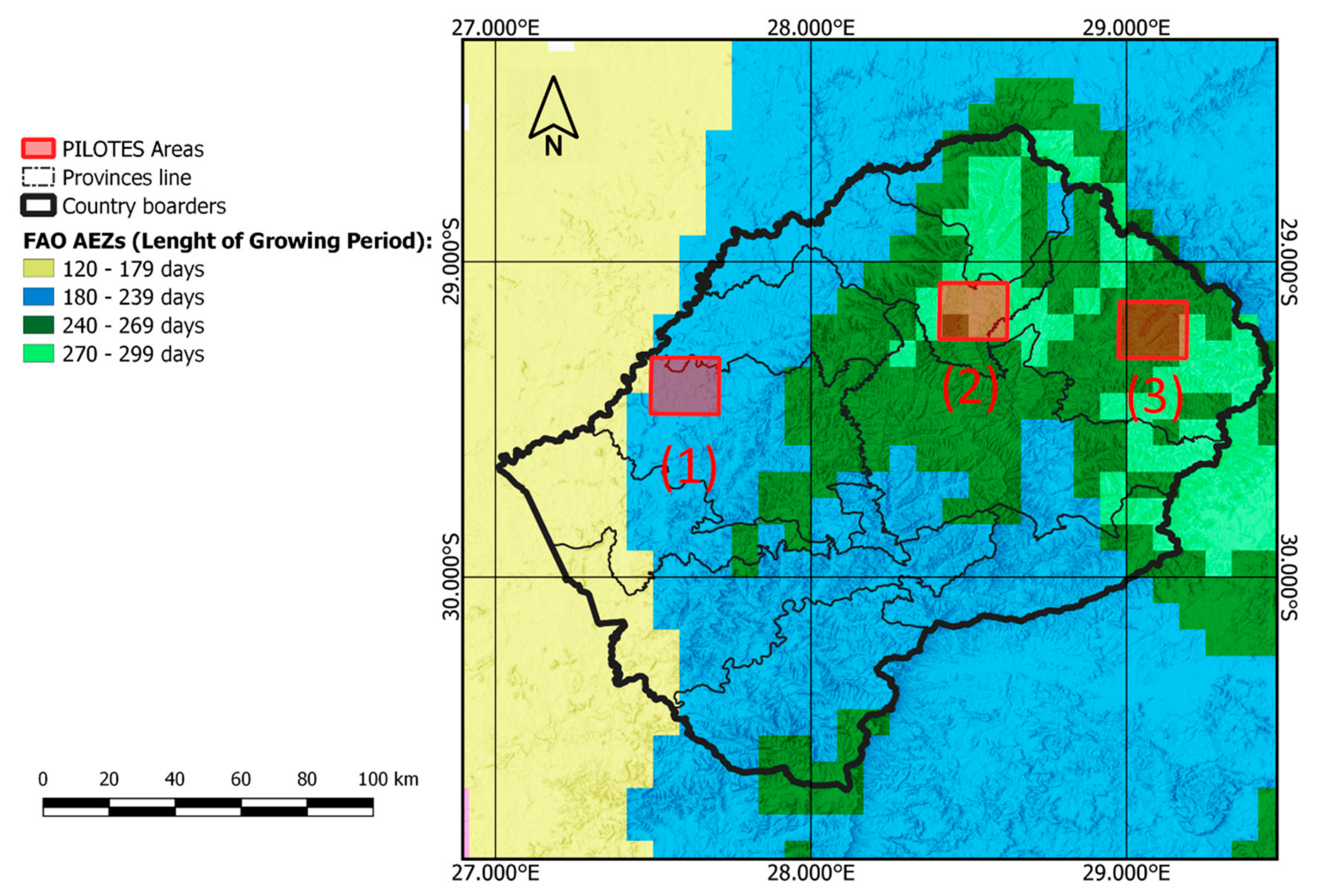
  • To evaluate the methodology on three different areas in Lesotho to ensure that it is independent from climatic variables and agro-ecological zones.
This paper is structured as follows: Section 2 describes the study areas and the data; Section 3 presents the proposed methods; Section 4 is dedicated to the results and Section 5 highlights the main findings and the implications of this study and is followed by our conclusion.

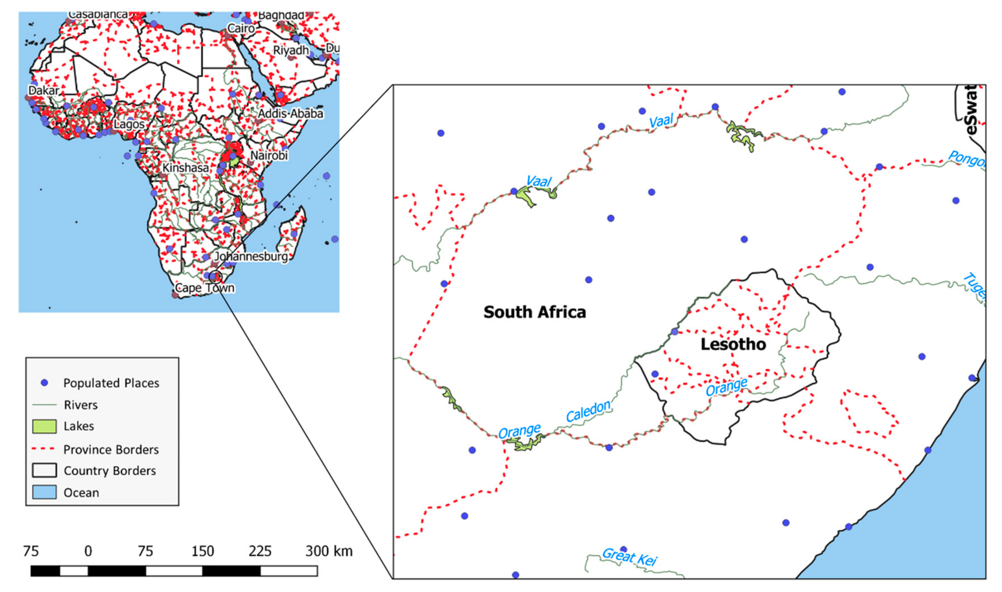
2. Study Area and Data

2.1. Study Area

This study has been carried out over territory of the Kingdom of Lesotho (Figure 1). The Kingdom of Lesotho is a landlocked country completely surrounded by South Africa. The total area of the country is 30,450 km2, making it the 137th largest country on the planet. Lesotho’s population was estimated to be 2,174,645 in 2015 by the UN and expected to reach 2,607,957 by 2030 and 3,203,470 by 2050 [1]. The poverty level in Lesotho is high with 62 percent of the population living on less than 2 USD per day. It is estimated that 36.4 percent are living on 1 USD or less per day. Agriculture is the main economic sector in Lesotho such that 60–70% of the country’s laborers obtain supplemental income from agriculture.
Poverty is the worst in rainfed farming areas. The country’s territory is divided into four agro-ecological zones based on altitude and landscape, namely: lowlands, the foothills, the Senqu River Valley (SRV), and the mountains [13]. The FAO Global Agro-Ecological Zones [31] divide the country into four major agro-ecological zones which are characterized by four different lengths of growing period (LGP) based on analysis of climate, soil, and terrain data (Figure 2).
The climate of Lesotho is characterized by two main seasons: a rainy season from October to the end of March and a dry season from April to the end of September. Normally the majority of precipitation occurs during the southern hemisphere summer thunderstorms (Figure 3).
In this study three different pilot areas labelled as (1) Maseru, (2) Lejone, and (3) Mokhotlong with surface areas of 482.65, 484.45, and 492.39 km2, respectively, were selected from the territories of Lesotho in a way that each area would fall within a distinct agro-ecological zone to represent Lesotho’s variability of different geological features, land cover and land use.
Footprints of the selected areas are shown in Figure 2. This will ensure the efficiency and the independency of the proposed algorithm for providing comprehensive training data. It is well-known that different agro-ecological zones form unique ecosystems influencing plant growth characteristics including photosynthesis (plant chlorophyll content) and therefore spectral reflection [32].

2.2. FAO Land Cover Lesotho Classes

FAO Land Cover of Lesotho (FAO LCL) was developed in 2016 using commercial satellite images and conventional GIS methods, along with supervised image classification techniques with very high-resolution satellite and airborne images with spatial resolution of 1.5 m. It utilizes an object-based classification on pan-sharpened images. The FAO LCL consists of 32 land cover categories based on FAO ISO 19144 Land Cover Meta Language, which provides a common reference structure for the comparison and integration of data for any generic land cover classification system [33]. A list of land cover classes and the specifications of satellite images that were used in FAO LCL data are shown in Table 1 and Table 2, respectively [34]. In this study, the FAO LCL resolution was resampled in order to change the spatial resolution from 1.5 m to 10 m so that it would match Sentinel 2 spatial resolution. The pixel values of the original dataset represented the dominant land cover for each land cover class within 10 m × 10 m cells. These values were aggregated across the new pixel size using a majority filter of 100 m × 100 m cell size. The majority filter algorithm determined the new value of the cell based on the most popular land cover within the filter window. Such method has been used by FAO in 2014 to harmonize national land cover datasets into the GLC-SHARE land cover and by other studies [6,35,36].

2.3. Test and Training Data Set Generation
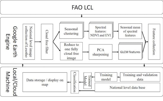
Machine learning (ML) models are often used to classify satellite images. In order to train the ML models, a set of ground truth labeled data points are required. In this study, we have randomly selected over 12,000 points from three pilot areas. To ensure that the accuracy measurements for all classifications are in the same order, the training and validation points were equally distributed between all land cover classes. FAO LCL was used for labelling the training points.

3. Methods

Figure 4 shows the workflow of the proposed methodology. First, the FAO LCL data was prepared and ingested into the GEE as data assets. Data preprocessing and feature extraction was done using GEE on cloud machine by utilizing GEE JavaScript API. All the available Sentinel-2 imagery between the first of October 2015 until the end of December 2017 were used as open access data. Images were preprocessed to remove cloudy pixels and formed (1) an image stack divided into four seasons and (2) a single image for all the territory of Lesotho. The image stack was used to extract the spectral features as explained in Section 3.2.1. The single image was sharpened using Principal Component Analysis (PCA) coefficients and then spatial features were extracted as explained in Section 3.2.2. Finally, the feature vectors of three pilot areas were exported for training, validation, and classification steps on local or cloud machines.

3.1. Google Earth Engine Data

In this regard, GEE was used to collect and extract data at the national level for Lesotho. First, all the available Sentinel-2 image tiles were selected for Lesotho and clipped to the country’s borders. Clouds were filtered based on a pixel-wise filtering technique by the band QA60 of Sentinel-2 products with a 5% cloudy pixel rate. This guaranteed that all the image tiles used in the next steps were only removing cloudy pixels of each image without removing the whole tile. Then image collection was divided into four groups based on the imagery season. Lesotho possesses four distinct seasons: spring-rainy season (October first to the end of December), summer-rainy season (January first to end of March), Autumn-dry season (April to end of June) and Winter-dry season (July to end of September). The season time periods are based on the data available on the Famine Early Warning Systems (FEWS) (www.fews.net) and the MODIS NDVI band (Figure 3).

3.2. Data Preparation

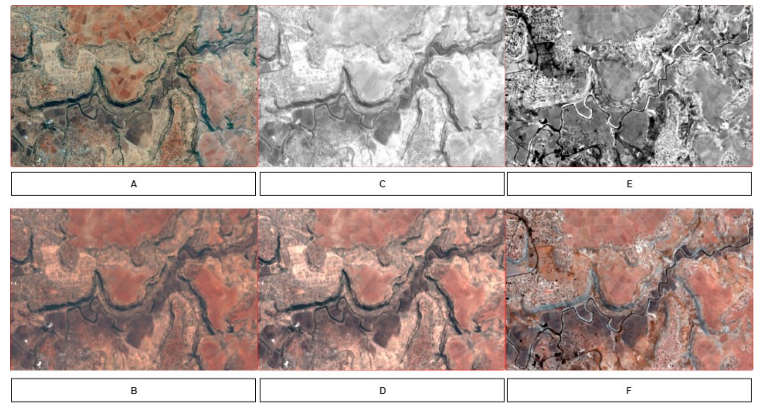
3.2.1. Spectral Features

High spectral resolution satellite sensors produce images in a higher number of bands in both visible and invisible spectrums with narrower bandwidth [34]. Higher spectral sensitivity of sensors could help in obtaining more information from earth surfaces including vegetation. One of the benefits of high spectral images is the possibility of calculating different vegetation indices (VI). VIs, which are obtained from satellite sensors, have been intensively studied and applied in many environmental and remote sensing studies. Xue et al. listed 118 different VIs and reviewed the most popular ones [37]. In this regard, the Normalized Vegetation Index (NDVI) is the most utilized VI, which was introduced by Rouse Jr. et al. [38] as follows:
N D V I = N I R R e d N I R + R e d
NDVI is sensitive to vegetation even in conditions of scarce vegetation. However, soil brightness, soil color, atmosphere, clouds, and shadows affect the NDVI. Since NDVI has negative correlation with soil brightness and atmospheric effect. Enhanced Vegetation Index (EVI) was later introduced which simultaneously correlates soil and atmospheric effects as:
E V I = G × N I R R e d N I R + C 1 × R e d C 2 × B l u e + L
where G is the gain factor equal to 2.5, L = 1 is the soil-adjustment factor, C1 = 6 and C2 = 7.5 are the coefficients of the aerosol resistance term, which uses the blue band to correct aerosol influences in the red band [39,40].
In this study, the seasonal mean of NDVI and EVI were calculated as spectral features based on Lesotho climatic seasons (Figure 3) on all existing data. The combined application of NDVI and EVI decreases the effect of atmospheric transmission and insures the reliability of the spectral features.

3.2.2. Spatial Features

In addition to the spectral properties of satellite images, the spatial properties (i.e., image texture) are important characteristics that can be used to describe land cover. Texture is defined as feel, appearance, or consistency of a surface or a substance. In the digital image processing field, the texture is the spatial arrangement of colors or pixel intensities. Different sets of metrics are designed in image processing to quantify the perceived texture of an image. Hereby, spatial properties were extracted from the Sentinel-2 images into two steps.

Image Pre-Processing with PCA

To extract the textural properties of images, it is necessary to pre-process the images in order to remove the noise or increasing the amount of details in each images tile. Therefore, to increase the differences between different textures in an image, principal component analysis (PCA) was applied.
PCA uses orthogonal transformation to convert possibly correlated data into linearly uncorrelated values so that the first principal component has the largest possible variance [41]. In general, almost any data matrix can be simplified by PCA. PCA estimates the correlation structure of variables. Therefore, principal component analysis of a data matrix extracts the dominant patterns in the matrix.
PCA was applied on visible channels (B2, B3, and B4) and near infrared (NIR) channel (B8) of Sentiel-2 images. Then the first component was combined with the original image plus a coefficient. Pan-sharpening is the injection of high-resolution panchromatic image into lower resolution multispectral images to get higher resolution multispectral images [42]. However, this study takes advantage of PCA pan-sharpening method on Sentinel-2 images by applying PCA coefficients that were obtained from visible bands and the bands with higher atmospheric transmission (i.e., band 8 and 12) on all the bands. Figure 5 compares the first and second principal components with Google Earth images, Sentinel-2 images and the final sharpening results using first and second components.

Texture Features: Grey Level Co-occurrence Matrix (GLCM)

A co-occurrence matrix is a matrix that is defined over an image I in which it is the distribution of co-occurring pixel values (grayscale values or colors) at a given offset Δ x , Δ y that is a position operator to be applied on any pixel in an image. The i , j t h value of the co-occurrence matrix gives the number of times in the image that the i t h , and j t h pixel values occur in the relation given by the offset. For an image with p different pixel values, the p × p co-occurrence matrix C is defined over an n × m image I , as:
C Δ x , Δ y i , j = x = 1 n y = 1 m 1 , i f   I x , y = i     a n d     I x + Δ x ,   y + Δ y = j 0 , o t h e r w i s e ,
where, I x , y indicates the pixel value at the pixel x , y . Here, the co-occurrence matrices were calculated over three visible and two NIR bands for an offset of 8 pixels distance in all directions.
Second order statistics can be derived from co-occurrence matrices to quantify the properties of an image. In this study, we have calculated 18 s-order statistics introduced by Haralick et al. and Conners et al., e.g., correlation, sum of variance, and contrast, etc. [43,44].

3.3. Trained Machine Learning Models

For machine learning models, we have trained bagged trees (BT) and support vector machine (SVM). BT and SVM have been used in various studies for land surface classification [45,46,47]. The BT that was used in this study is an ensemble of decision trees model with 30 learner trees [48]. The BT model in this study only accepts one parameter (number of trees). It should be noted that, typically, in remote sensing applications, random forest classifiers are used which are a specific type of bagged trees in which it needs two parameters. First, the number of trees, and second is the number of features (predictors) to train each decision tree. However, in this study, the BT model was trained on all features. The SVM model was trained based on a degree three polynomial kernel [49] and one verses one (ovo) decision function.

4. Results

4.1. Trained Models’ Performance

Table 3 shows the overall accuracy and training time for both models. The training time for the SVM model was significantly higher than the BT model. The BT and SVM were trained and validated based on a randomly generated dataset (12,000 point). BT yielded a higher overall accuracy in a 5-fold cross validation process.
Both models were trained and validated on a laptop PC with 1.8 GHz dual-core Intel Core i5 CPU and 8 GB of memory to demonstrate the efficiency and practicality of the proposed method in real world scenarios. Training and segmentation steps in remote sensing applications require high computational power as well as memory resources [7,18]. In this study, the training time for both models showed very high efficiency despite the size of the training and validation datasets. Furthermore, the achieved time efficiency would allow the users to modify or add ground truth data samples and to retrain the models in the future. This will guarantee the operational ability of the algorithm.
Table 4 and Table 5 show the confusion matrices for the BT and SVM models. The BT achieved highest accuracy, in the built-up class, 81%, while the SVM gained the highest accuracy in the hydrology class, 76%. The differences of models’ performance were not significant in the agriculture, tree and barren-land classes. The lowest accuracy was observed in shrub-land and grass-land classes for both models. However, in the case of in grass-land class, the BT showed a lower score than the SVM. The ESA CCI 20 m land cover of Africa reported an overall accuracy of 65%, however, the overall accuracy for Lesotho was reported between 22% and 45%. The proposed methodology in this research out-performed the ESA CCI 20 m land cover by 20% [12].

4.2. Classes Accuracy and Inter-Class Similarities

Table 4 and Table 5 also shows the highest confusion rate for each class. It should be noted that both ML models had high confusion rates in similar classes. The built-up class allocated the highest confusion rate in agriculture and grass-land classes with 6% and 5% for the BT model and 8% and 15% for the SVM model, respectively. Similarly, the highest confusion rate for the agriculture class was observed in the grass-land class with 11% and 13% for the BT and SVM, respectively.
Tree and shrub-land classes showed a 13% and 9% confusion rate where the tree class was selected as shrubs or vice versa. Also, the highest confusion rate for shrub-lands was occurred in grass-land class with 17%. Grass-land class has the highest confusion rates with other classes with 17%, 14%, and 13% for shrub-land, barren-land, and agricultural areas respectively.

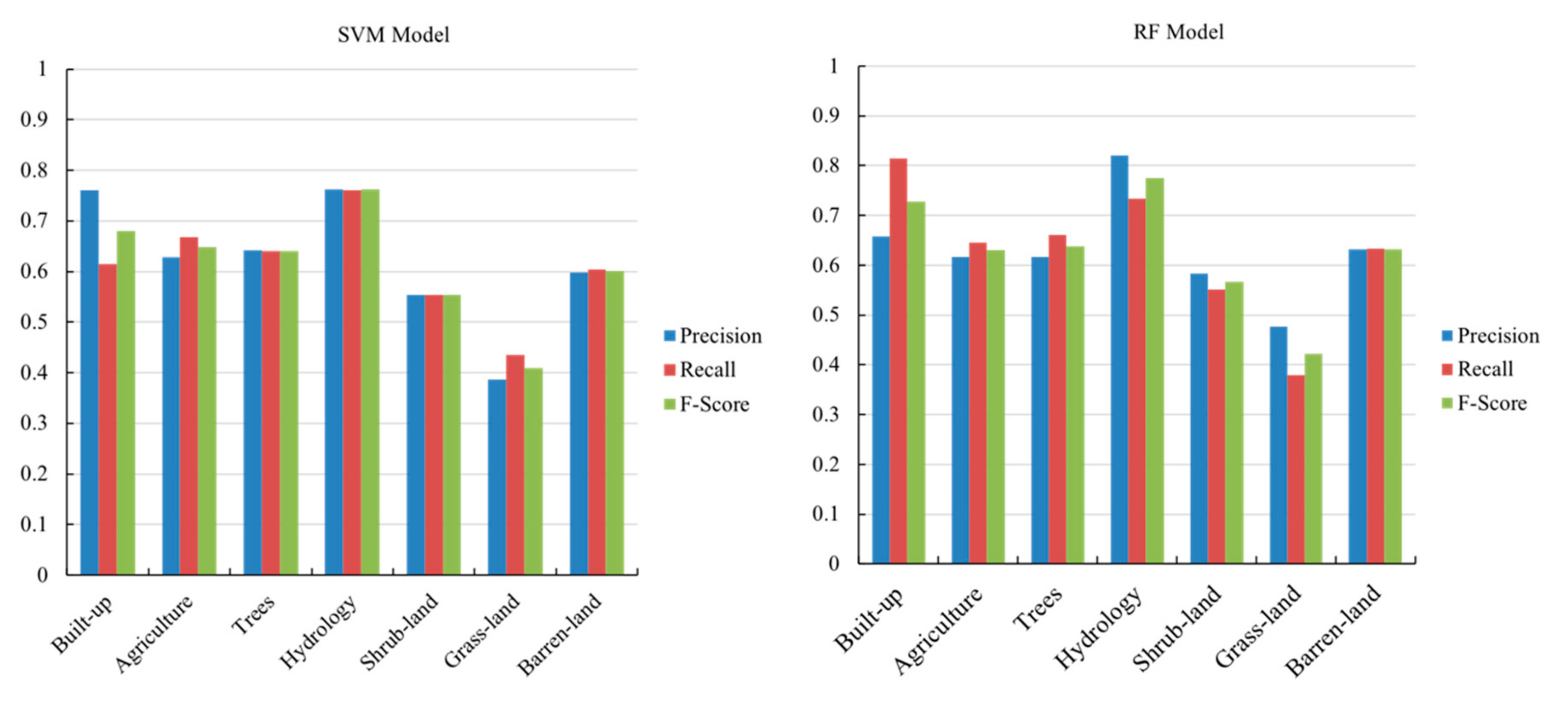
4.3. Discriminating Ability of the Train Models: Precision, Recall, and Receiver Operator Curve

Figure 6 shows the recall, precision and F-score values for both trained models. As can be seen in this figure, both models have similar precision and recall values. Precision is the fraction of relevant points among the retrieved points in a specific class, while recall is the fraction of relevant points that is retrieved over the total amount of relevant points in a class. Our results indicate that both models are successful in retrieving relevant classes for both in-sample and out-sample data. Precision comparing false positives to true positives. It captures the effect of the large number of negative examples on the model’s performance, while higher recall means that the trained model is successful in returning most of the relevant results [50].
Figure 7 compares the recall, area under the curve (AUC) in a receiver operator curve (ROC), and a false positive rate (FPR) for both ML models. When comparing the AUC values of trained models, the BT model showed higher ability in retrieving relevant data than the SVM. Also, the false positive rate for both models was very low, meaning the number of incorrect points that were assigned to each class of the land cover was low.

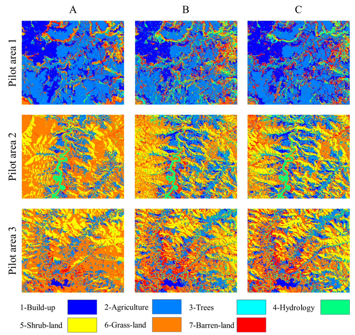
4.4. Classification Results and Final Land Cover Product

The trained models were tested on the selected pilot areas to generate the final land cover products. The testing step was run on the same PC as training and validation step. Segmentation results for studied pilot areas are shown in Figure 8. The images in column A show the FAO LCL as the base map for training ML models. Images in columns B and C show the results for the SVM and BT models, respectively. The BT model classified the pilot areas in average 51 min for each pilot area. The BT model was 48% faster than those of SVM in classifying pilot areas.

5. Discussion

5.1. Google Earth Engine as a Cloud Base Remote Sensing Platform

GEE was able to calculate the feature vector for the entire territory of Lesotho. Computational power of GEE enables feature extraction at the national level; however, it was out of computation-time in some circumstances. It could be due to high dimensional matrix operations for PCA analysis and GLCM passing the system limits on allowed processing time for each request [18]. This problem can be avoided by extracting the features at a local level instead of a national level, once the initial parameters for PCA (i.e., the mean and covariance of pixel values for the selected bands) were extracted for the country’s territory. GEE allows processing of data through its APIs in different ways. However, this study selected the JavaScript API and GEE code editor as the main data processing tool. The goal was to minimize the cost and increase the time efficiency of GEE in land cover mapping. Meanwhile, the processing of generated feature vectors required to be partly executed on cloud machine (i.e., GEE), then exported and partly processed on the local machine (PC), since such processing method was causing the GEE code editor to run out of computation-time. This process of exporting and processing the feature vector on a local/cloud machine acts as the main bottleneck of the algorithm’s pipeline. Further efforts are required to overcome this problem by using new GEE features in the future.

5.2. The Effect of Spectral and Spatial Features on Accuracy Performance

Image segmentation has traditionally been applied to single-date satellite images [51]. Several studies report the advantages of satellite time series segmentation, such as automated detection of agricultural fields [50], better and faster forest change analysis [51], robustness against shadowing and registration errors [51,52], reduced salt-and-pepper effect apparent in per-pixel classifications [53], and the segmentation of multi-temporal images for cropland mapping [9]. In this study, we trained the ML models based on the mean of a two years’ period in order to allow the ML models to learn the spectral and temporal features of different land cover classes. Therefore, the proposed methodology successfully takes advantage of the power of multi-temporal satellite time series, but still has the flexibility to deliver accurate land cover products on an annual base period for land cover and land use change applications.
Nyland et al. and Xiong et al. used GEE for land cover mapping by using fully spectral features of available satellite time series [8,11]. However, using a times series introduces a level of confusion to the final land cover products since the land cover is subject to change during the time, i.e., a landscape could vary from forest to agriculture in due time because of agricultural development [7]. In this study, we attempted to overcome this problem by using the GEE’s potentials in extracting texture features of land surfaces in addition to spectral features for the first time. Introducing spatial (texture) features as a descriptor for land cover mapping enabled our proposed method to perform on an annual base process. It means the method needs the data of one annual period to be able to predict land cover classes. The experiment showed that in the case of Lesotho the same method performs with 40% and 51% overall accuracy by utilizing only spectral or spatial features, respectively. On the other hand, when utilizing the GLCM in a feature vector, it is important to select the spatial distance parameter in the GLCM offset relative to the resolution of the satellite images. Therefore, the effect of GLCM parameters in land cover mapping applications ask for more investigation in future studies.

5.3. The Inter-Class Confusion Rates

In 2017, Inglada et al. reported a high confusion between continuous and discontinuous urban fabrics. However, our study out performed their results with 81% accuracy for the BT model it is noteworthy that in this study, all continuous and discontinuous urban fabrics were merged into the built-up class [7]. The confusion between the built-up, agriculture and grass-land classes happened in two major situations: first, in areas where the built-up class contains large abandoned land between buildings and second in areas where small agricultural activities occur in cites or rural areas.
Moreover, agricultural lands were selected as grass-land in areas with higher soil moisture content. These areas are mainly located near wet-lands such as areas near springs, slopes or at the bottom of valleys. The vegetation growth in these areas is more continuous and in similar temporal patterns with natural vegetation [9]. Also, confusion between agriculture and grass-land was common in rainfed and sloping lands where natural vegetation and crops have similar growth periods. These results can also be confirmed based on the Table 1 definition of each class.
Shrubs (0.5~1.5 m height) and trees (1.5 m~ height) normally have very similar growth patterns and similar spatial distribution. These similarities will result in almost identical spectral and spatial characteristics for trees and shrubs. In addition, shrub-lands in FAO LCL data are defined as open shrubs with natural vegetation in between, which could lead to confusion between shrub-land and grass-land classes. Moreover, the two classes are containing bare rocks or areas without any vegetation and therefore were classified as barren-land.
The earth surface geometry influences the quality of segmentation [54]. Meanwhile, woody shrubs naturally grow on surfaces toward the south while natural vegetation is more adopted to areas with shorter daylight time [55]. Therefore, the surface geometry typically affects the type of land cover in each area. As an example, this effect could be seen in the final map product (Figure 7) where the shrub-lands are located mostly on areas sloping toward the south. The comparison between the FAO LCL and visual inspections results showed that the study results are more compatible with pilot areas’ topology and geometry.
The proposed methodology was able to provide an accurate land cover of urban and agriculture lands. These land cover products are based on continuously updating satellite data with an annual cycle. Such annually based product will allow the authorities in the country to monitor urban and agriculture lands in line with the indicator 2.4.1 of SDGs to measuring the proportion of agricultural area within productive and sustainable agriculture [4].

6. Conclusions

In this paper, an operational land cover mapping methodology is presented based on available free access Sentinel-2 data and the GEE cloud processing platform. By utilizing a combination of GEE and the FAO LCL data, our main objective was to measure the performance of machine learning models and classify the land surface by using high dimensional feature space. The validation with the proposed method and satellite imagery revealed an accuracy of 62 and 67%, respectively, for the important land cover categories such as ‘urban’ and ‘agricultural lands’. Moreover, the trained models provided a precise land cover tool for annual land cover and land use change comparison applications. The models were trained, validated and tested on a simple laptop PC to demonstrate the cost and time efficiency of the methodology. Such methodology opens doors for in field processing and mapping land cover for future studies.
The study showed the GEE potentials in land cover mapping by processing the feature vector at a national level for Lesotho in a short time. Further investigation is required to unveil the ability of GEE in applying new ML techniques, i.e., deep learning models, on geospatial data. The current GEE pipeline for processing the available data on GEE through the Python or JavaScript APIs requires exporting large volumes of data to cloud or local storage as well as running the ML models on a cloud machine. These processes are time consuming and require extra funds for cloud processing and cloud storage.
Knowing the scale of the country, moderate resolution of the images, and natural changes and errors in FAO LCL as the base map, the proposed methodology achieved accuracy that could be considered satisfactory. Therefore, it is hoped that the individuals and organizations involved in rural and urban development strategies, as well as forest and land conservation at regional and sub-regional scales, can utilize the presented models for developing countries as an alternative to traditional higher-cost GIS methods.

Author Contributions

Conceptualization, M.M., H.M. and T.S.; Formal analysis, M.M., H.M., L.D.S. and T.S.; Investigation, M.M.; Methodology, M.M., L.D.S. and T.S.; Software, M.M.; Supervision, L.D.S., S.V., N.K. and T.S.; Validation, M.M., S.V. and T.S.; Writing—original draft, M.M., H.M. and T.S.; Writing—review & editing, M.M., H.M., S.V., N.K. and T.S.

Funding

This research was funded by the Ministry of Education, Culture, Sports, Science and Technology (MEXT) of Japan [a Grant-in-Aid for Scientific Research (KAKENHI) (No. 17K19965) and the Leading Graduate School for Green and Clean Food Production, Tokyo University of Agriculture and Technology research fellowship.

Acknowledgments

We are sincerely grateful to Mbuli Charles Boliko, director of the FAO Liaison Office in Japan and the FAO Headquarters, Rome, Italy for supports during the research and providing FAO LCL which was used in this research.

Conflicts of Interest

The authors declare no conflict of interest.

References

  1. Nations, U. World population prospects: The 2015 revision. U. N. Econ. Soc. Aff. 2015, 33, 1–66. [Google Scholar]
  2. Kamwi, J.M.; Chirwa, P.W.; Manda, S.O.; Graz, P.F.; Kätsch, C. Livelihoods, land use and land cover change in the Zambezi Region, Namibia. Popul. Environ. 2015, 37, 207–230. [Google Scholar] [CrossRef] [Green Version]
  3. Nations, U. Resolution adopted by the General Assembly on 25 September 2015. In Transforming Our World: The 2030 Agenda for Sustainable Development; United Nations: New York, NY, USA, 2015. [Google Scholar]
  4. United-Nations. Sustainable Development Goals Indicators. Available online: https://unstats.un.org/sdgs/metadata/files/Metadata-02-04-01.pdf (accessed on 23 May 2019).
  5. Gómez, C.; White, J.C.; Wulder, M.A. Optical remotely sensed time series data for land cover classification: A review. ISPRS J. Photogramm. Remote Sens. 2016, 116, 55–72. [Google Scholar] [CrossRef] [Green Version]
  6. Latham, J.; Cumani, R.; Rosati, I.; Bloise, M. Global Land Cover Share (GLC-SHARE) Database Beta-Release Version 1.0-2014; FAO: Rome, Italy, 2014. [Google Scholar]
  7. Inglada, J.; Vincent, A.; Arias, M.; Tardy, B.; Morin, D.; Rodes, I. Operational high-resolution land cover map production at the country scale using satellite image time series. Remote Sens. 2017, 9, 95. [Google Scholar] [CrossRef]
  8. Nyland, E.K.; Gunn, E.G.; Shiklomanov, I.N.; Engstrom, N.R.; Streletskiy, A.D. Land Cover Change in the Lower Yenisei River Using Dense Stacking of Landsat Imagery in Google Earth Engine. Remote Sens. 2018, 10, 1226. [Google Scholar] [CrossRef]
  9. Belgiu, M.; Csillik, O. Sentinel-2 cropland mapping using pixel-based and object-based time-weighted dynamic time warping analysis. Remote Sens. Environ. 2018, 204, 509–523. [Google Scholar] [CrossRef]
  10. Cardille, J.A.; Fortin, J.A. Bayesian updating of land-cover estimates in a data-rich environment. Remote Sens. Environ. 2016, 186, 234–249. [Google Scholar] [CrossRef]
  11. Xiong, J.; Thenkabail, P.S.; Gumma, M.K.; Teluguntla, P.; Poehnelt, J.; Congalton, R.G.; Yadav, K.; Thau, D. Automated cropland mapping of continental Africa using Google Earth Engine cloud computing. ISPRS J. Photogramm. Remote Sens. 2017, 126, 225–244. [Google Scholar] [CrossRef] [Green Version]
  12. Lesiv, M.; Fritz, S.; McCallum, I.; Tsendbazar, N.; Herold, M.; Pekel, J.F.; Buchhorn, M.; Smets, B.; van de Kerchove, R. Evaluation of ESA CCI Prototype Land Cover Map at 20m; International Institute for Applied Systems Analysis: Laxenburg, Austria, 2017. [Google Scholar]
  13. Hachigonta, S.; Nelson, G.C.; Thomas, T.S.; Sibanda, L.M. Southern African Agriculture and Climate Change: A Comprehensive Analysis; International Food Policy Research Institute: Washington, DC, USA, 2013. [Google Scholar]
  14. Mumby, P.; Green, E.; Edwards, A.; Clark, C. The cost-effectiveness of remote sensing for tropical coastal resources assessment and management. J. Environ. Manag. 1999, 55, 157–166. [Google Scholar] [CrossRef]
  15. Ridder, R.M. Global forest resources assessment 2010: Options and recommendations for a global remote sensing survey of forests. FAO For. Resour. Assess. Programme Work. Pap. 2007, 141. Available online: http://www.fao.org/3/a-ai074e.pdf (accessed on 23 May 2019).
  16. UN FAO. GeoNetwork Opensource Portal to Spatial Data and Information. Available online: http://www.fao.org/geonetwork/srv/en/main.home (accessed on 30 July 2019).
  17. Stibig, H.J.; Belward, A.S.; Roy, P.S.; Rosalina-Wasrin, U.; Agrawal, S.; Joshi, P.K.; Beuchle, R.; Fritz, S.; Mubareka, S.; Giri, C. A land-cover map for South and Southeast Asia derived from SPOT-VEGETATION data. J. Biogeogr. 2007, 34, 625–637. [Google Scholar] [CrossRef]
  18. Gorelick, N.; Hancher, M.; Dixon, M.; Ilyushchenko, S.; Thau, D.; Moore, R. Google Earth Engine: Planetary-scale geospatial analysis for everyone. Remote Sens. Environ. 2017, 202, 18–27. [Google Scholar] [CrossRef]
  19. European-Space-Agency. Copernicus Data Access Policy. Available online: https://www.copernicus.eu/en/about-copernicus/international-cooperation (accessed on 23 May 2019).
  20. Woodcock, C.E.; Allen, R.; Anderson, M.; Belward, A.; Bindschadler, R.; Cohen, W.; Gao, F.; Goward, S.N.; Helder, D.; Helmer, E. Free access to Landsat imagery. Science 2008, 320, 1011. [Google Scholar] [CrossRef] [PubMed]
  21. Loveland, T.R.; Dwyer, J.L. Landsat: Building a strong future. Remote Sens. Environ. 2012, 122, 22–29. [Google Scholar] [CrossRef]
  22. Hansen, M.C.; Potapov, P.V.; Moore, R.; Hancher, M.; Turubanova, S.; Tyukavina, A.; Thau, D.; Stehman, S.; Goetz, S.; Loveland, T.R. High-resolution global maps of 21st-century forest cover change. Science 2013, 342, 850–853. [Google Scholar] [CrossRef] [PubMed]
  23. Pekel, J.F.; Cottam, A.; Gorelick, N.; Belward, A.S. High-resolution mapping of global surface water and its long-term changes. Nature 2016, 540, 418. [Google Scholar] [CrossRef] [PubMed]
  24. Lobell, D.B.; Thau, D.; Seifert, C.; Engle, E.; Little, B. A scalable satellite-based crop yield mapper. Remote Sens. Environ. 2015, 164, 324–333. [Google Scholar] [CrossRef]
  25. Dong, J.; Xiao, X.; Menarguez, M.A.; Zhang, G.; Qin, Y.; Thau, D.; Biradar, C.; Moore, B., III. Mapping paddy rice planting area in northeastern Asia with Landsat 8 images, phenology-based algorithm and Google Earth Engine. Remote Sens. Environ. 2016, 185, 142–154. [Google Scholar] [CrossRef] [PubMed] [Green Version]
  26. Patel, N.N.; Angiuli, E.; Gamba, P.; Gaughan, A.; Lisini, G.; Stevens, F.R.; Tatem, A.J.; Trianni, G. Multitemporal settlement and population mapping from Landsat using Google Earth Engine. Int. J. Appl. Earth Obs. Geoinf. 2015, 35, 199–208. [Google Scholar] [CrossRef] [Green Version]
  27. Zhang, Q.; Li, B.; Thau, D.; Moore, R. Building a better urban picture: Combining day and night remote sensing imagery. Remote Sens. 2015, 7, 11887–11913. [Google Scholar] [CrossRef]
  28. Coltin, B.; McMichael, S.; Smith, T.; Fong, T. Automatic boosted flood mapping from satellite data. Int. J. Remote Sens. 2016, 37, 993–1015. [Google Scholar] [CrossRef] [Green Version]
  29. Huang, H.; Chen, Y.; Clinton, N.; Wang, J.; Wang, X.; Liu, C.; Gong, P.; Yang, J.; Bai, Y.; Zheng, Y. Mapping major land cover dynamics in Beijing using all Landsat images in Google Earth Engine. Remote Sens. Environ. 2017, 202, 166–176. [Google Scholar] [CrossRef]
  30. Sidhu, N.; Pebesma, E.; Câmara, G. Using Google Earth Engine to detect land cover change: Singapore as a use case. Eur. J. Remote Sens. 2018, 51, 486–500. [Google Scholar] [CrossRef]
  31. Fischer, G.; Nachtergaele, F.O.; Prieler, S.; Teixeira, E.; Tóth, G.; van Velthuizen, H.; Verelst, L.; Wiberg, D. Global Agro-Ecological Zones (GAEZ v3. 0)-Model Documentation; IIASA: Laxenburg, Austria; FAO: Rome, Italy, 2012. [Google Scholar]
  32. Mokarram, M.; Sathyamoorthy, D. Modeling the relationship between elevation, aspect and spatial distribution of vegetation in the Darab Mountain, Iran using remote sensing data. Model. Earth Syst. Environ. 2015, 1, 30. [Google Scholar] [CrossRef]
  33. Nations, FaAOoTU. ISO19144-2: Geographic Information Classification Systems—Part 2: Land Cover Meta Language (LCML); International Organization for Standardization (ISO): Geneva, Switzerland, 2012. [Google Scholar]
  34. The United Nations, FAO. Land Cover Atlas of Lesotho; FAO: Rome, Italy, 2017. [Google Scholar]
  35. Campbell, J.B. Introduction to Remote Sensing, Virginia Polytechnic Institute and State University; The Guildford Press: New York, NY, USA, 1996. [Google Scholar]
  36. Vancutsem, C.; Marinho, E.; Kayitakire, F.; See, L.; Fritz, S. Harmonizing and combining existing land cover/land use datasets for cropland area monitoring at the African continental scale. Remote Sens. 2013, 5, 19–41. [Google Scholar] [CrossRef]
  37. Xue, J.; Su, B. Significant remote sensing vegetation indices: A review of developments and applications. J. Sens. 2017, 2017, 1–17. [Google Scholar] [CrossRef]
  38. Rouse, J.W., Jr.; Haas, R.; Schell, J.; Deering, D. Monitoring vegetation systems in the Great Plains with ERTS. 1974. Available online: https://ntrs.nasa.gov/search.jsp?R=19740022614 (accessed on 13 August 2019).
  39. Jiang, Z.; Huete, A.R.; Didan, K.; Miura, T. Development of a two-band enhanced vegetation index without a blue band. Remote Sens. Environ. 2008, 112, 3833–3845. [Google Scholar] [CrossRef]
  40. A Database for Remote Sensing Indices. Available online: https://www.indexdatabase.de/db/s-single.php?id=96 (accessed on 23 May 2019).
  41. Wold, S.; Esbensen, K.; Geladi, P. Principal component analysis. Chemom. Intell. Lab. Syst. 1987, 2, 37–52. [Google Scholar] [CrossRef]
  42. Shah, V.P.; Younan, N.H.; King, R.L. An efficient pan-sharpening method via a combined adaptive PCA approach and contourlets. IEEE Trans. Geosci. Remote Sens. 2008, 46, 1323–1335. [Google Scholar] [CrossRef]
  43. Conners, R.W.; Trivedi, M.M.; Harlow, C.A. Segmentation of a high-resolution urban scene using texture operators. Comput. Vis. Gr. Image Process. 1984, 25, 273–310. [Google Scholar] [CrossRef]
  44. Haralick, R.M.; Shanmugam, K. Textural features for image classification. IEEE Trans. Syst. Man Cybern. 1973, 3, 610–621. [Google Scholar] [CrossRef]
  45. Hao, P.; Zhan, Y.; Wang, L.; Niu, Z.; Shakir, M. Feature selection of time series MODIS data for early crop classification using random forest: A case study in Kansas, USA. Remote Sens. 2015, 7, 5347–5369. [Google Scholar] [CrossRef]
  46. Mountrakis, G.; Im, J.; Ogole, C. Support vector machines in remote sensing: A review. ISPRS J. Photogramm. Remote Sens. 2011, 66, 247–259. [Google Scholar] [CrossRef]
  47. Mardani, M.; Fujii, Y.; Saito, T. Detection and Mapping of Hairy Vetch in Images Obtained by UAVs. In Proceedings of the International Workshop on Image Electronics and Visual Computing, Da Nang, Vietnam, 28 February–3 March 2017. [Google Scholar]
  48. Breiman, L. Bagging Predictors; Report No. 421; Univ. California: Pasadena, CA, USA, 1994. [Google Scholar]
  49. Boser, B.E.; Guyon, I.M.; Vapnik, V.N. A training algorithm for optimal margin classifiers. In Proceedings of the 5th Annual ACM Workshop on Computational Learning Theory, Pittsburgh, PA, USA, 27–29 July 1992; pp. 144–152. [Google Scholar]
  50. Davis, J.; Goadrich, M. The relationship between Precision-Recall and ROC curves. In Proceedings of the 23rd international conference on Machine learning, Pittsburgh, PA, USA, 25–29 June 2006; pp. 233–240. [Google Scholar]
  51. Desclée, B.; Bogaert, P.; Defourny, P. Forest change detection by statistical object-based method. Remote Sens. Environ. 2006, 102, 1–11. [Google Scholar] [CrossRef]
  52. Mäkelä, H.; Pekkarinen, A. Estimation of timber volume at the sample plot level by means of image segmentation and Landsat TM imagery. Remote Sens. Environ. 2001, 77, 66–75. [Google Scholar] [CrossRef]
  53. Matton, N.; Canto, G.; Waldner, F.; Valero, S.; Morin, D.; Inglada, J.; Arias, M.; Bontemps, S.; Koetz, B.; Defourny, P. An automated method for annual cropland mapping along the season for various globally-distributed agrosystems using high spatial and temporal resolution time series. Remote Sens. 2015, 7, 13208–13232. [Google Scholar] [CrossRef]
  54. Yan, L.; Roy, D. Automated crop field extraction from multi-temporal Web Enabled Landsat Data. Remote Sens. Environ. 2014, 144, 42–64. [Google Scholar] [CrossRef] [Green Version]
  55. Daubenmire, R. Mountain topography and vegetation patterns. Northwest Sci. 1980, 54, 146–152. [Google Scholar]
Figure 1. The Kingdom of Lesotho (study area) within the continent of Africa.
Remotesensing 11 01907 g001
Figure 2. Agro-ecological zones of Lesotho based on length of growing period (LGP) and foot-print of pilot areas. (1) Maseru, (2) Lejone, and (3) Mokhotlong.
Remotesensing 11 01907 g002
Figure 3. Comparison between mean of normalized difference vegetation index (NDVI) of three studied pilot areas and agricultural seasons in Lesotho.
Remotesensing 11 01907 g003
Figure 4. Algorithm workflow of proposed machine learning classification and accuracy assessment methodology.
Remotesensing 11 01907 g004
Figure 5. (A) Google Earth high resolution image. (B) Sentinel-2 10-m resolution image. (C) First principal component of 4 selected bands. (D) PCA sharpened image with first principal component. (E) Second component of PCA. (F) Sharpened image with second component of PCA.
Remotesensing 11 01907 g005
Figure 6. Precision, recall and F-Score parameters for each class. Left: Support Vector Machine model. Right: Bagged Trees model.
Remotesensing 11 01907 g006
Figure 7. Area under curve (AUC) values in receiver operator curve (ROC), recall, and false positive rate per class for trained models.
Remotesensing 11 01907 g007
Figure 8. Comparison between the pilot areas 1, 2 and 3 for (A): FAO land cover of Lesotho (FAO LCL), (B): Results of trained SVM model and (C): Results of BT model.
Remotesensing 11 01907 g008
Table 1. FAO LCL classes and classes definitions.
Class CodeLC TypeLC NameLC Description
1BUILT-UP (4 classes)Urban AreasRelatively larger urban built-up areas, commonly with presence of trees
Urban Commercial and/or Industrial areasCommercial and/or industrial built-up areas
Rural Settlements, Plain Areas Rural houses in flat lying plain areas + small cultivated herbaceous crops + closed herbaceous natural vegetation, often together with trees and/or shrubs employed for demarcation
Rural Settlements, Slopping and Mountain AreasRural houses in sloping and mountainous areas + herbaceous natural vegetation, occasionally with shrubs employed for demarcation, usually treeless
2AGRICULTURE (5 Classes)Rainfed Agriculture, Plain AreasRainfed herbaceous crops cultivated in flat-lying plains, relatively larger sized fields
Rainfed Agriculture, Sloping & Mountainous regions Rainfed herbaceous crops in sloping land and mountains with terracing and/or contour ploughing, small and medium sized fields, sometimes with lines of shrubs demarcating fields
Rainfed Agriculture, Sheet ErosionRainfed herbaceous crops with visible water sheet erosion, commonly with associated gully erosion
Irrigated AgricultureSmall size irrigated herbaceous crops near water courses
Rainfed Agriculture + Rainfed Orchards Small rainfed herbaceous crops + regular rainfed orchard plantations (usually as rows of fruit trees separating elongated fields)
3TREES (7 Classes)Trees, Needle leaved, (Closed)Closed evergreen needle-leaved trees, sometimes occurring as plantations
Trees, Needle leaved, (Open)Open evergreen needle-leaved trees + herbaceous natural vegetation
Trees, Broadleaved, (Closed)Closed deciduous broadleaved trees, commonly along river beds
Trees, Broadleaved, (Open)Open deciduous broadleaved trees + herbaceous natural vegetation
Trees, Undifferentiated (Closed)Closed undifferentiated trees
Trees, Undifferentiated, (Open)Open undifferentiated trees + herbaceous natural vegetation
Trees, (Sparse)Sparse trees + herbaceous natural vegetation (closed-open)
4HYDROLOGY (4 Classes)Large WaterbodyLarge perennial fresh water lake or dam reservoir
Small WaterbodySmall fresh water seasonal and/or perennial reservoir, Pool, Waterhole, etc.
Wetland (Perennial and/or seasonal)Natural perennial and/or seasonal fresh waterbody + Perennial closed-open natural vegetation
River BankRiver Bank (soil/sand deposits) + perennial or periodic flowing fresh water (river)
5SHRUBLAND (2 Classes)Shrub-land-(Closed)Natural Shrubs (H = 0.5 to 1.5 m), Closed
Shrub-land-(Open)Natural Shrubs (H = 0.5 to 1.5 m), Open + Natural herbaceous vegetation (Open Closed)
6GRASSLAND (1 Class)GrasslandGrassland—Natural vegetation
7BARREN LAND (5 Classes)Bare RockRock outcrops
Bare AreaBare areas—undifferentiated areas not used for cultivation and usually devoid of grass or shrub cover
Boulders & Loose RocksAreas with large scattered boulders and/or unconsolidated loose rocks, commonly sloping, usually together with patchy natural vegetation and/or shrubs and/or natural trees
GulliesGully erosion, occasionally with trees and/or tall shrubs
Mines & QuarriesMajor mines and quarries as well as temporary building material extraction sites
Table 2. FAO LCL specifications of utilized images.
Image SourceSpatial Resolution (Meter)Spectral Resolution
Rapid Eye55 bands (440 to 850 nm)
Spot 52.55 Bands (480 to 1750 nm)
Aerial orthophotos0.53 Bands (visible light)
Table 3. Results of the overall accuracy.
ClassifierTraining Time (Seconds)Over-All Accuracy (%)
Bagged Trees7662.6
Support Vector Machine119760.4
Table 4. Confusion Matrix—Bagged Trees Model (%).
Class No.Class NameBuilt-UpAgricultureTreesHydrologyShrub-LandGrass-LandBarren-Land
1Built-up81631153
2Agriculture965226115
3Trees1036631143
4Hydrology67573243
5Shrub-land46131551110
6Grass-land111553143814
7Barren-land76338963
Table 5. Confusion Matrix—Cubic SVM Model (%).
Class No.Class NameBuilt-UpAgricultureTreesHydrologyShrub-LandGrass-LandBarren-Land
1Built-up628532155
2Agriculture567235136
3Trees426441384
4Hydrology26476255
5Shrub-land259255179
6Grass-land51344174314
7Barren-land373491460

