Article

Towards Automated Ship Detection and Category Recognition from High-Resolution Aerial Images

1
Institute of Electronics, Chinese Academy of Sciences, Beijing 100190, China
2
Key Laboratory of Network Information System Technology (NIST), Institute of Electronics, Chinese Academy of Sciences, Beijing 100190, China
3
School of Electronic, Electrical and Communication Engineering, University of Chinese Academy of Sciences, Beijing 100190, China
*
Author to whom correspondence should be addressed.
Remote Sens. 2019, 11(16), 1901; https://doi.org/10.3390/rs11161901
Submission received: 25 July 2019 / Accepted: 7 August 2019 / Published: 14 August 2019
(This article belongs to the Special Issue Convolutional Neural Networks Applications in Remote Sensing)

Abstract

:
Ship category classification in high-resolution aerial images has attracted great interest in applications such as maritime security, naval construction, and port management. However, the applications of previous methods were mainly limited by the following issues: (i) The existing ship category classification methods were mainly to classify on accurately-cropped image patches. This is unsatisfactory for the results of the existing methods in practical applications, because the location of the ship in the patch obtained by the object detection varies greatly. (ii) The factors such as target scale variations and class imbalance have a great influence on the performance of ship category classification. Aiming at the issues above, we propose a novel ship detection and category classification framework. The category classification is based on accurate location. The detection network can generate more precise rotated bounding boxes in large-scale aerial images by introducing a novel Sequence Local Context (SLC) module. Besides, three different ship category classification networks are proposed to eliminate the effect of scale variations, and the Spatial Transform Crop (STC) operation is used to get aligned image patches. Whatever the problem of insufficient samples or class imbalance have, the Proposals Simulation Generator (PSG) is considered to handle this properly. Most remarkably, the state-of-the-art performance of our framework is demonstrated by experiments based on the 19-class ship dataset HRSC2016 and our multiclass warship dataset.

Graphical Abstract

1. Introduction

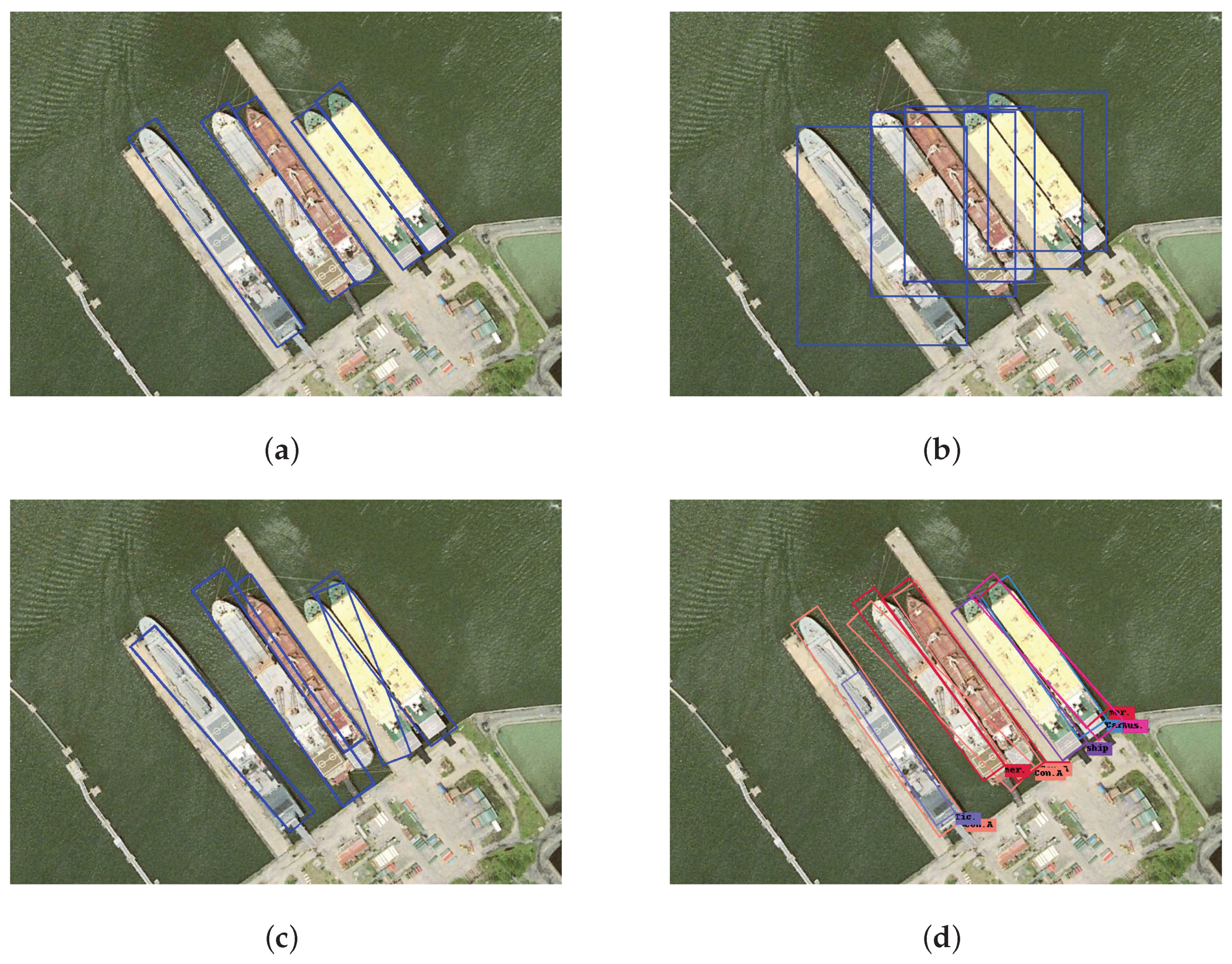
Ship detection and recognition in high-resolution aerial images are challenging tasks, which play an important role in many related applications, e.g., maritime security, naval construction, and port management. Although many ship classification methods have been proposed, they only roughly identify the ship as warship, container ship, oil tanker, etc., on the accurate image patch. However, what is needed to know for us is the more specific ship categories like Arleigh Burke, Perry, Ticonderoga, etc., and it is difficult to obtain high-quality sample patches by automatic ship detection. Some methods have tried to locate ships and identify their categories at the same time; nevertheless, the results are undesirable such that they lead to serious confusion, as shown in Figure 1d.
Existing research on ship detection and classification can be divided into two aspects. One is the location problem, which finds the ships in the aerial images and expresses the location in some way. The other is the classification issue, which assigns the ships to different categories.
Object detection is a fundamental and challenging task in computer vision, aimed at determining whether there are any instances of targets in an image or not. In the field of remote sensing, ship and ship wake detection have attracted considerable attention of researchers. Iervolino et al. [1] proposed a ship detector based on the Generalized Likelihood Ratio Test (GLRT) to improve the detection ability under low signal-to-noise/clutter ratios. The GLRT algorithm has proven to be effective and has been extensively used in [2,3,4]. Graziano et al. [5] exploited the Radon Transform (RT) to detect ship wake and validated the method’s robustness in [6]. Biondi et al. [7,8,9] first utilized the Low-Rank plus Sparse Decomposition (LRSD) algorithm assisted by RT to achieve excellent performance on ship wake detection. The inclination of ships also can be calculated by LRSD and RT for some regions of interest [10].
Recently, with the development of Deep Convolutional Neural Networks (DCNN) [11], an increasing number of efficient ship detection frameworks have been reported [12,13,14,15,16]. Zou et al. [12] proposed a novel SVD Network (SVDNet) based on the convolutional neural networks and the singular-value decompensation algorithm to learn features adaptively from remote sensing images. Huang et al. [14] proposed Squeeze Excitation Skip-connection Path networks (SESPNets) to improve the feature extraction capability for ship detection and used soft Non-Maximum Suppression (NMS) to avoid deleting some correct bounding boxes for some targets. However, these methods are based on the Horizontal Bounding Box (HBB). Although this representation has no effect on the sparse targets at sea, it is not suitable for densely-docked inshore vessels. As shown in Figure 1b, the angle of the ship can be in an arbitrary direction, and the aspect ratio of the ship is large, so the horizontal bounding box of one ship may contain a relatively large redundancy region, which is not conducive to the classification task. Therefore, we chose the representation shown in Figure 1a.
With the improvement of the resolution of aerial images, more and more works have tried to detect inshore vessels and use the Rotated Bounding Box (RBB) to locate ships [17,18,19,20]. Liu et al. [17] proposed the Rotated Region-based CNN (RR-CNN) to predict rotated objects and changed the Region of Interest (RoI) pooling layer in order to extract features only from the rotation proposal. Zhang et al. [18] modified the Faster R-CNN [21] and utilized the Rotation Region Proposal Networks (RRPN) [22] and the Rotation Region of Interest (RRoI) Pooling layer to detect arbitrarily-oriented ships. Yang et al. [19] proposed Rotation Dense Feature Pyramid Networks (RDFPN) to solve problems resulting from the narrow width of the ship and used multiscale RoIAlign [23] to solve the problem of feature misalignment. However, the above networks ignored one problem that is important for classification. As shown in Figure 1c, when the background is complex and the ships are densely docked, the rotated bounding box cannot accurately locate the ship. If the box is too small, the discriminative regions such as prow that are important for classification will be missed. If the box is too large, it will contain the background and the adjacent ships, which is not conducive to classification either. In order to better classify the ships into different categories, we must attach importance to how to generate more precise rotated ship bounding boxes. In other words, we do not meet the situation where the Intersection over Union (IoU) value is only greater than 0.5. Therefore, based on the arbitrarily-oriented ship detection network, we introduce the Sequence Local Context (SLC) module to predict more accurate rotated bounding boxes.
As for the ship category classification task, most methods are concentrated on a few large ship categories with distinctive features [24,25,26,27]. Wu et al. [26] proposed a model named BDA-KELM, which combines Kernel Extreme Learning Machine (KELM) and the dragonfly Algorithm in Binary Space (BDA) to conduct the automatic feature selection and search for optimal parameter sets to classify the bulk carrier, container ship, and oil tanker. Some works tried to classify more types of ships. Oliveau et al. [27] trained a nonlinear mapping between low-level image features and the attribute space to build discriminative attribute representations. Based on these attributes, a Support Vector Machine (SVM) classifier is built for the classification of image patches into 12 categories. However, these traditional methods need careful design and extraction of complex features, which increases the computational complexity. Motivated by advanced CNN models, such as VGGNet [28], GoogleNet [29], and DenseNet [30], CNN models have been used in ship classification in high-resolution aerial images. Bentes et al. [31] built a CNN model with four convolutional layers, four pooling layers, and a fully-connected layer to achieve good performance among the five categories of targets. However, previous methods on ship classification whether using traditional methods or based on the CNN model both concentrated on a few large categories of ships and achieved classification based on accurately-cropped image patches. To solve these problems, in this work, we achieve the classification of 19 classes of ships with large differences in scale and characteristics based on the patches from the output of our ship detector. The work most similar to ours is that of Ma et al. [32]. However, they used a horizontal bounding box, which cannot handle the inshore vessels and only classified sparse ships in the sea with a single background into eight categories.
In conclusion, the challenges of ship detection and classification in high-resolution aerial images are mainly in the following three aspects: (i) It is an important basis for classification to find as many ships as possible and predict accurate target locations, especially including the most discriminative regions and excluding noise information (background and the part of adjacent targets). (ii) The size of the different types of ships varies greatly, which is not conducive to classification. (iii) The scarcity of training data causes class imbalance, which can result in overfitting to more frequent ones and ignoring the classes with a limited number of samples.
In this paper, based on the challenges above, we propose a rotation-based ship detection network to capture accurate location and three different ship category classification networks to solve the problem of large difference in ship scale. Finally, a Proposals Simulation Generator (PSG) is introduced to address the problem of insufficient samples and class imbalance. The main contributions of this paper are as follows:
  • We build a new rotation-based ship detection network. The trade-off between recall and precision is different compared with the previous ship detection methods such that the recall rate is ensured with the condition of high precision.
  • The SLC module is introduced to extract local context features, which makes the rotated bounding box fit tightly with the ship. The accurate bounding box can include the discriminative parts such as prow and exclude noise information such as background.
  • In order to reduce the burden of the classification network, we introduce the Spatial Transform Crop (STC) operation to obtain aligned image patches. Aiming at the problem of the large difference in ship scale, we propose three different ship category classification networks.
  • A PSG is designed to greatly augment the training data by simulating the output style of the ship detector, which can address the problem of insufficient samples and class imbalance.
  • We achieve state-of-the-art performances on two real-world datasets for ship detection and classification in high-resolution aerial images. The phenomenon of category confusion like Figure 1d does not appear, and it is considered more suitable for practical application.
The rest of this paper is organized as follows: Section 2 describes the details of the proposed method. In Section 3, we describe the datasets and present experiments to validate the effectiveness of the proposed algorithm. Section 4 discusses the results of the proposed method. Finally, Section 5 concludes this paper.

2. Materials and Methods

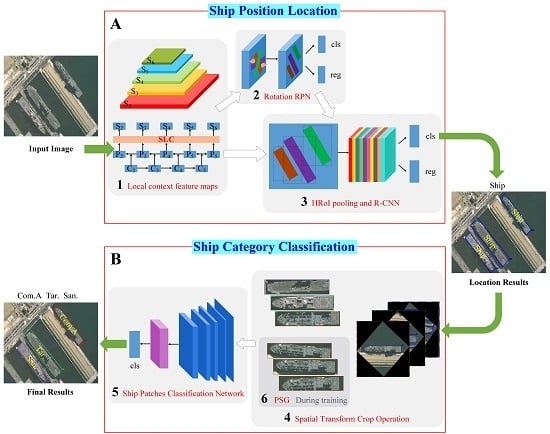
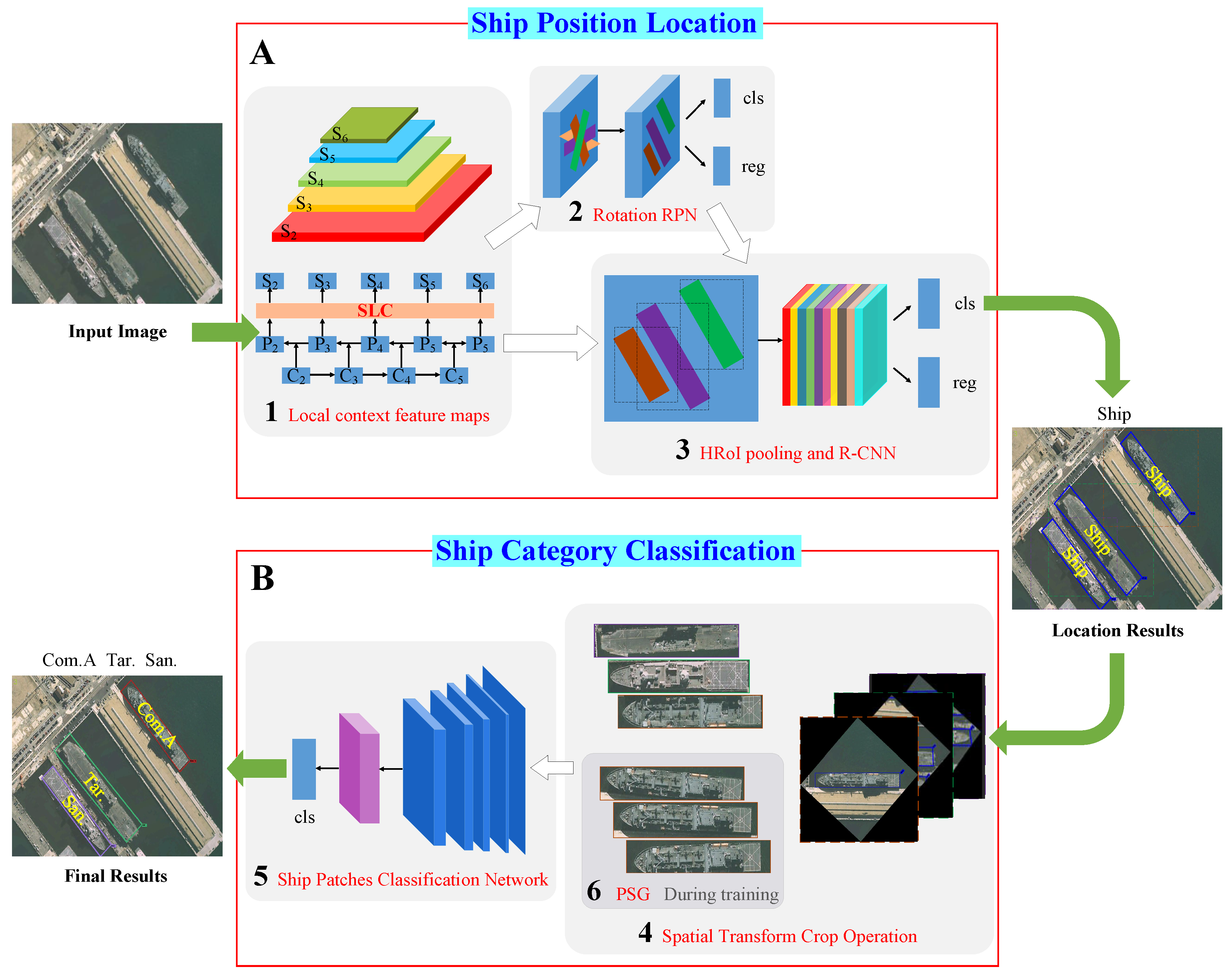
The pipeline of our proposed framework is illustrated in Figure 2. The whole system is mainly divided into two phases: the location phase and the classification phase. Give an input image with size m × n , the ship location is first obtained through the red box A, and then, the red box B is used to get the category of each ship target. The computational Block Number 1 extracts the local context feature maps with size m / s × n / s , where s is the output stride. Block Number 2 regards the feature maps as input and outputs a set of rotated rectangular object proposals, each with an objectness score. We randomly sampled 256 proposals in an image to compute the loss function. The computational Block Number 3 crops and resizes the feature maps inside these proposals into the fixed spatial extent by max pooling (such as 14 × 14 ) and outputs the ship location. Block Number 4, which is used to crop and resize the ship regions from the input image to the same size, does not participate in the training process. Finally, the computational Block Number 5 takes the ship regions as input and outputs the specific ship categories such as Arleigh Burke, Perry, Ticonderoga, etc. Block Number 6, which is used in the training process, generates large training samples to address the problem of insufficient annotated pictures. In our framework, the computational Block Numbers 1, 2, 3, and 5 are devoted to training the model, and Block Numbers 4 and 6 are dedicated to decoding features. Subsequently, the main parts of our framework are presented in detail.

2.1. Rotation Proposals and HRoI Pooling Layer

In most object detection tasks, the ground-truth of the object is described by the horizontal bounding box with ( x , y , w , h ) , where ( x , y ) is the center of the bounding box, and the width w and height h represent the long side and the short side of the horizontal bounding box, respectively [33]. However, the bounding box represented in this way cannot perfectly outline the strip-like rotated ship. In our task, the rotated bounding box with five tuples ( x , y , w , h , θ ) was introduced to represent the location of the ship, and the parameter θ (between zero and 180) describes the angle from the horizontal direction of the standard bounding box.
Similar to the way of RRPN, we added the angle parameter outside of the scale and aspect ratio to generate the rotation anchors. The value of the angle parameter was defined as 0 , π 3 , 2 π 3 . The zero means generating the horizontal anchors, and the other two generate oriented anchors. In addition, as ships always have special shapes, we analyzed the shape of the ship targets in the dataset and refer to the setting of the relevant work [18,34,35,36,37]. We set 1:3, 1:7 as the aspect ratios. The scale of anchors were set from 32–512 by a multiple of two on different Feature Pyramid Networks (FPN) [38] layer. An extra anchor scale of 1.414 was introduced on each layer to reduce the spacing of the scale [39]. In summary, for each point on different feature maps of FPN, 12 rotation anchors (3 angles, 2 aspect ratios, and 3 scales) were generated, and the total number of anchors on the feature map with height H and width W was 12 × H × W . For the rotated bounding boxes regression, we adopted smooth L 1 loss [40] for the rotation proposals:
L r e g d * , d = i x , y , w , h , θ s m o o t h L 1 d i * d i
s m o o t h L 1 x = 0.5 x 2 i f x < 1 x 0.5 o t h e r w i s e
where variables d and d * represent the detection proposal and ground-truth label, respectively. The five coordinates of d and d * are calculated as follows:
d x = x x a w a , d y = y y a h a d w = l o g w w a , d h = l o g h h a , d θ = θ θ a
d x * = x * x a w a , d y * = y * y a h a d w * = l o g w * w a , d h * = l o g h * h a , d θ * = θ * θ a
where variables x , x a , and x * are for the predicted box, anchor box, and ground-truth box, respectively, and the variables y , w , h , θ are the same. The operation α β = α β + k π , k Z rescales the angle within the range ( π 2 , π 2 ] .
For the rotation proposals, the traditional IoU computation method cannot obtain the IoU value accurately to distinguish whether it is a positive rotation proposal or a negative rotation proposal. The skew IoU computation method was introduced to solve this problem. We divided the convex polygon of intersection points set into multiple triangles by the triangulation [41] and calculated the area of each triangle. Then, the sum of the areas was the IoU value.
The arbitrarily-oriented object detection methods always use the RRoI pooling layer to extract features of object regions accurately [18,19,
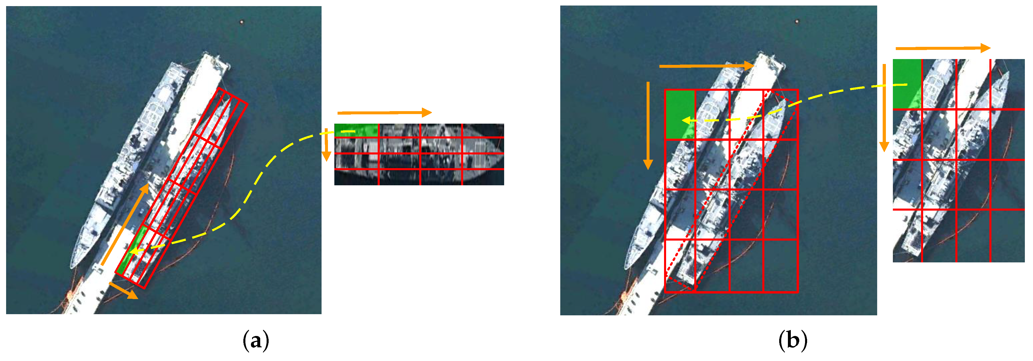
42]. As a hypothesis, we set the RRoI layer hyper-parameters to H r and W r . The rotated ship proposal region can be divided into H r × W r subregions of h / H r × h / W r size for a proposal with height h and width w (as shown in Figure 3a). Then, max pooling was performed in every subregion, and max-pooled values were saved in the matrix of each RRoI. This operation is very common in high-resolution aerial images like DOTA [43] and NWPUVHR-10 [44] to eliminate the mismatching between RRoIs and corresponding objects for classification and regression. In general, the RRoI pooling layer should be used for our detection network. However, different from other arbitrarily-oriented object detection, we did not need to classify the ships into more specific categories like Arleigh Burke, Perry, Ticonderoga, etc. Our detection network only needed to distinguish whether the proposal was a target or not. We hoped the ship detection network could achieve a higher recall rate, which is a different choice for the trade-off between recall and precision compared with other methods. Although the RRoI pooling layer can reduce the influence of the irrelevant background and other incomplete ships, the large aspect ratio of the ship may lead to misalignment of the rotating bounding box, resulting in a lower recall rate. In contrast, the Horizontal Region of Interest (HRoI) pooling layer [21,45] can extract more features, such as the features of ship shadows and adjoining ships, which can improve the target confidence and recall rate. Therefore, we applied the HRoI pooling layer, as shown in Figure 3b. We calculated the horizontal bounding box of the rotation proposal, then the HRoI pooling layer used max pooling to crop and resize the feature map inside the horizontal bounding box into the fixed spatial extent of h r × w r , where h r and w r are layer hyper-parameters. Finally, through the cls branch and reg branch, we obtained the predicted result, i.e., either ship or background.

2.2. Sequence Local Context Module

The features of high layers have strong semantics and of low layers have accurate location information. The FPN structure makes use of the feature hierarchy of a convolutional network, which combines the advantages of different layers via a top-down path to make all features have strong classification and regression capability. However, as shown in Figure 1, it was not enough for the ships densely docked in the harbor, and we hoped our network could distinguish the pixels belonging to different ships to predict a more accurate position. An intuitive idea is to learn the local context information around the objects based on the FPN structure. In our previous work [
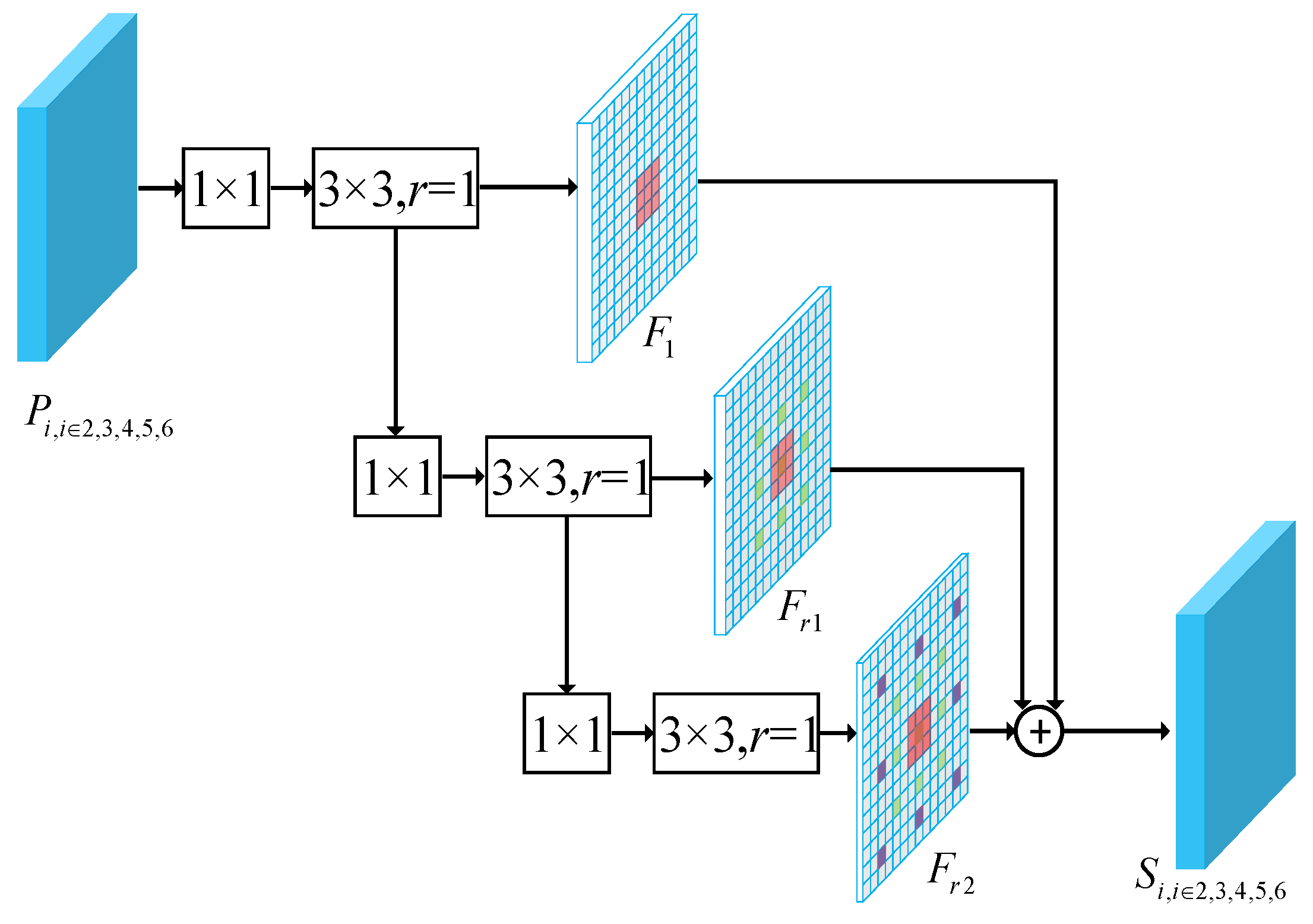
46], a flexible module called the sequence local context module was proposed to learn multi-scale local context features. Specifically, we utilized the dilated convolution with different dilation rates to integrate multi-scale context features. As shown in Figure 4, the SLC module consisted of three sequence convolutional blocks, each with a 1 × 1 convolution followed by a 3 × 3 dilated convolution with different dilation rates. The SLC module captures context information at different scales and fuses the outputs of three layers by element-wise summation operation. The module can be formulated as follows:
S L C = F 1 F , θ 1 + F r 1 F 1 , θ r 1 + F r 2 F r 1 , θ r 2
where F is the input feature and F 1 , F r 1 , F r 2 are the functions of convolution blocks with dilation rates 1, r 1 , r 2 , respectively. F 1 , F r 1 are the output features of F 1 , F r 1 . θ 1 , θ r 1 , and θ r 2 are respective parameters, and S L C is the output feature. The SLC module progressively enhances the connection of context information from different blocks and avoids losing too much information caused by the dilation rate.
In order to distinguish the adjacent ships and provide accurate locations for the second phase, we added the SLC module r 1 = 2 , r 2 = 3 after the FPN structure to make the features learn the local context information. The reason is as follows: Firstly, the module was proven to be effective at ship detection tasks. Secondly, the feature size of the input and of the output from the SLC module were identical, so it could be embedded between any two convolutional layers and did not require major modifications. By the way, this was another reason to apply the HRoI pooling layer, because the RRoI pooling layer could not extract the local context feature learned by the SLC module. The SLC module took the feature P i , i 2 , 3 , 4 , 5 , 6 from the FPN structure as input and output the feature S i , i 2 , 3 , 4 , 5 , 6 .

2.3. Spatial Transform Crop Operation

With the increase in the categories of ship classification, the type of ship becomes complex and highly similar, especially for smaller ships. Without the corresponding expertise, it is difficult for humans to distinguish between different types of ships. Therefore, it is necessary to build a classification network to better identify categories of different ships.
The STC operation was introduced to crop the rotated bounding boxes from the corresponding images, which can eliminate the noise information and align ship patches to better extract marginal visual differences between different types of ships. The detailed operation can be seen in Algorithm 1. Therefore, the detection part did not need to classify the different ships. The phenomenon of category confusion like Figure 1d did not appear. We only needed to consider the NMS within classes, not the NMS between classes [17].
Algorithm 1: Spatial Transform Crop (STC) algorithm.
Remotesensing 11 01901 i001

2.4. Ship Category Classification

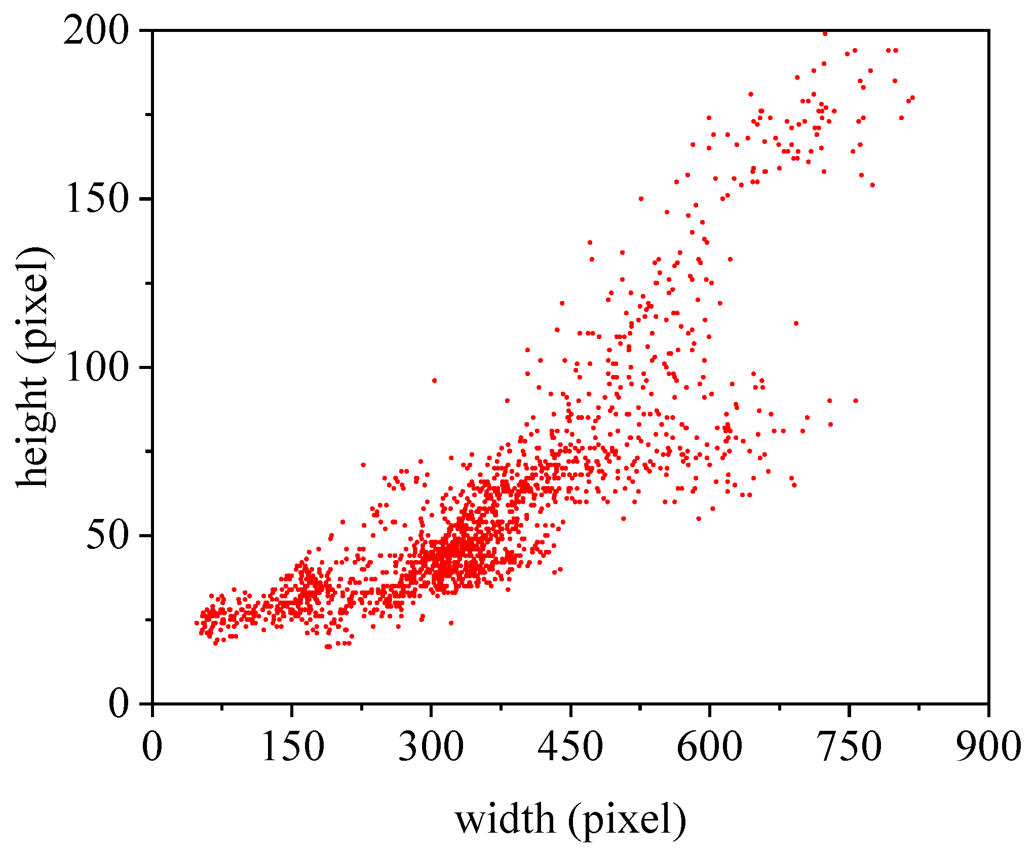
After STC operation, we found that the size of the patches was not uniform, because the length and width of different types of ships varied widely (as shown in Figure 5). However, the traditional classification networks needed a fixed-size input image, because the fully-connected layers required a fixed-size/-length input. The most intuitive method to handle this problem is that we resized the patches to the fixed size for the classification network. In general, this operation may reduce the recognition accuracy. In SPP-Net [47], the Spatial Pyramid Pooling layer is proposed to generate fixed-length representations regardless of image size/scale, which was proved to achieve much better classification results. However, could this similar operation work well in our task?
The objects with the same category, such as cats, dogs, and birds, may present large appearance variations due to changes of posture or viewpoints, complex backgrounds, and occlusions [48]. For example, the appearance of one bird can be very different when it is preying, resting, or flying, which makes intra-class variance great. The operation of resizing can exacerbate this situation to reduce the recognition accuracy. However, in aerial images, a powerful prior constraint is that we can only get the top view of targets, which makes our analysis easier. In addition, the ship is a rigid body, and we used the rotated bounding box. Therefore, it was unnecessary for us to consider the impact of the above factors. We propose the view that in high-resolution aerial images, the operation of resizing may produce a smaller negative impact than other operations.
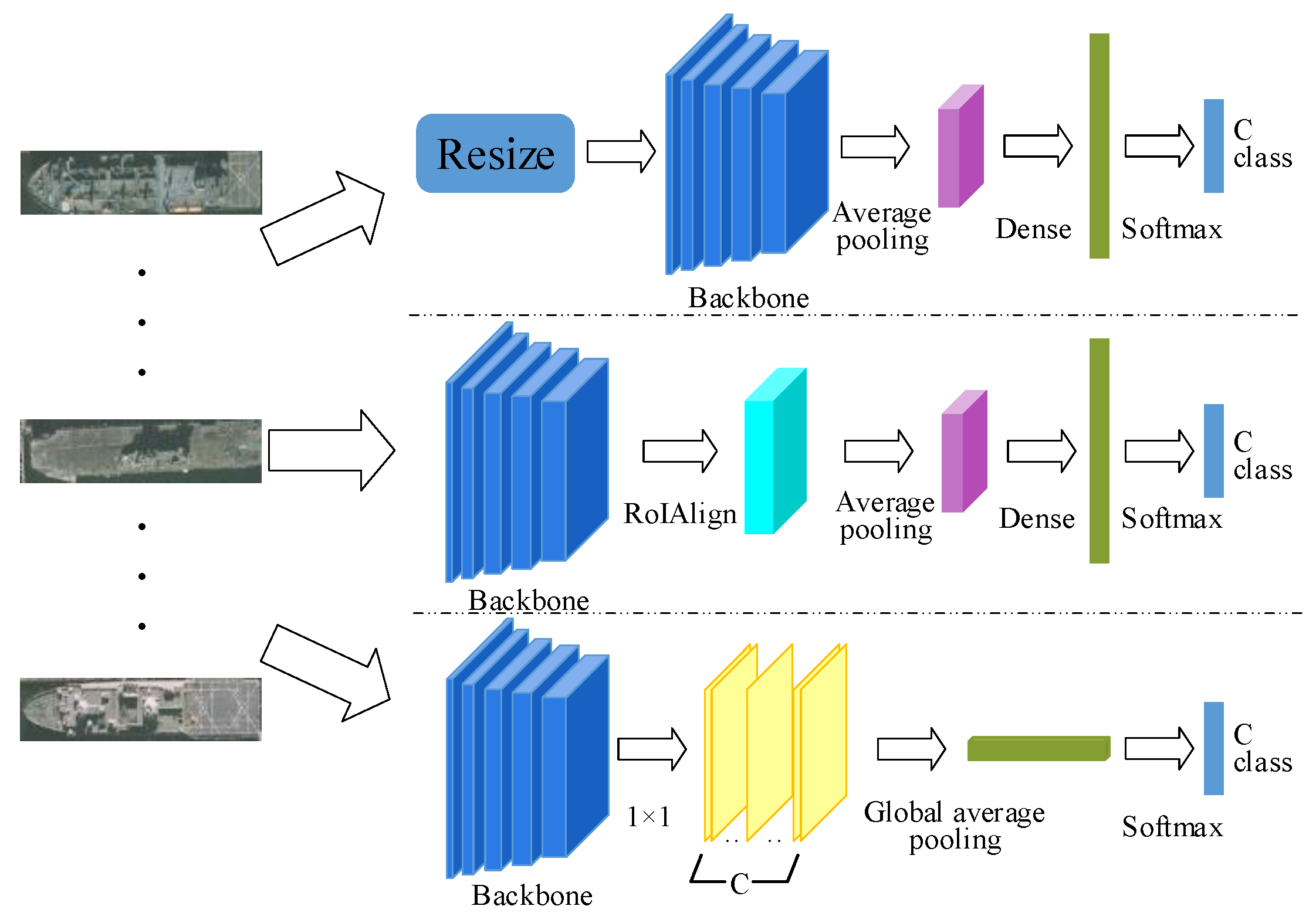
In order to verify our idea, in this paper, we propose three different methods to compare the effects of fixed-size and arbitrarily-sized input images on recognition accuracy. As shown in Figure 6, the classification network took the ship patches as input and output the specific ship categories such as Arleigh Burke, Perry, Ticonderoga, etc. For the first row, we fit the patches to the fixed size and then extracted the feature maps using the backbone network. The average pooling layer was introduced to reduce the feature dimension and preserve the important features. Finally, the fully-connected layers output the predicted class. The second row did not require a fixed patch size. We introduced the RoIAlign layer, which can aggregate the feature maps of the backbone network to meet the requirement of fully-connected layers. The third row was to use only a convolutional network like FCN [49] and ACoL [50]. We removed the fully-connected layers and added a convolutional layer of C (C is the number of classes) channels with the kernel size of 1 × 1, stride one on top of the feature maps. Then, the output was fed into a Global Average Pooling (GAP) layer followed by a softmax layer for classification. The conclusion will be elaborated in Section 3.2.2.

2.5. Proposals Simulation Generator

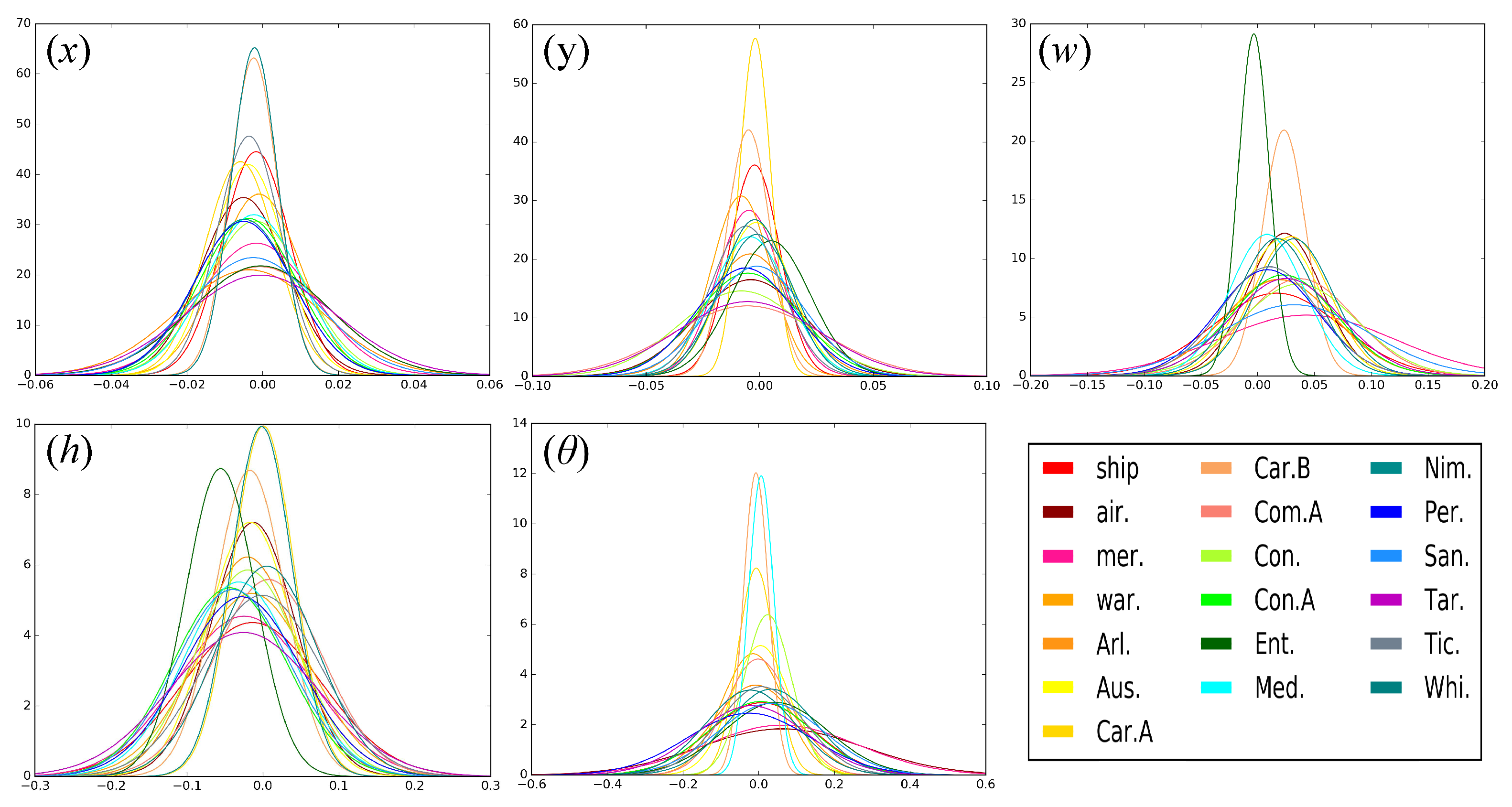
Due to insufficient training samples, the number of instances belonging to different types of ship would be unbalanced, and even several ship types would have very few samples. A proper data augmentation was necessary to increase the training samples and avoid the class imbalance. Since we already had the ground-truth box and predicted box for each ship, we could generate a large training sample with the same distribution as the predicted box. In this way, we could solve the above problems and improve the performance of our network.
Due to the different sizes and characteristics of different types of ships, we analyzed the distribution of the relative offsets between the predicted proposal and the ground-truth proposal for each class. Since the ship in the aerial images was a rigid body and oriented upward, it was simple to learn the distribution P δ f | T , where δ f represents the offset between the coordinates of the predicted proposal and the coordinates of the ground-truth proposal and T is the ground-truth proposal for each ship. For each proposal, we calculated the offsets between its ground-truth bounding proposal and detected bounding proposal. The offsets were then normalized by the corresponding coordinate of the ground-truth. After these operations, we fit the offset to a Gaussian distribution and show it in Figure 7.
During the training phase of the classification network, for each sample in the training set, we could generate many different offsets based on the distribution P δ f | T to obtain large augmented training samples.

3. Experiments and Results

In this section, we first introduce the evaluation datasets and then analyze the effectiveness of the different components for our framework. Finally, we compare our results with the previous methods.

3.1. Datasets

We choose two datasets to experiment with our framework in high-resolution aerial images. One was the public multiclass ship dataset HRSC2016 [51], and the other was our constructed dataset Multiclass Warship Collection (MWC).
HRSC2016 [51]: The dataset contained 1061 images with resolutions between 2 m and 0.4 m. The image sizes ranged from 300 × 300 1500 × 900 , and most of them were larger than 1000 × 600 . It contained 436 training images with 1207 instances, 181 validation images with 541 instances, and 444 testing images with 1228 instances. The label of the dataset included three levels, namely ship class (L1), ship category (L2), and ship type (L3), which contained 1 class, 4 classes, and 19 classes, respectively. The specific ship categories included ship (ship), aircraft carrier (air.), war craft (war.), merchant ship (mer.), Nimitz class aircraft carrier (Nim.), Enterprise class aircraft carrier (Ent.), Arleigh Burke class destroyer (Arl.), Whidbey Island class landing craft (Whi.), Perry class frigate (Per.), Sanantonio class amphibious transport dock (San.), Ticonderoga class cruiser (Tic.), Austen class amphibious transport dock (Aus.), Tarawa class amphibious assault ship (Tar.), Container ship (Con.), Command ship (Com.A), Car carrier A (Car.A), Container ship A (Con.A), Medical ship (Med.), Car carrier B (Car.B). The difference between Car.A and Car.B is shape. The bow and stern of Car.A are round, and the stern of Car.B is flat. The Con. and Con.A are designed for different applications. Con. is used to transport containers, and Con.A is used to transport other goods. In this work, we focused on the L3 classification. For a fair comparison, we excluded submarine, hovercraft classes, and samples with “different” labels, as done in [17].
MWC: We collected 934 aerial images with resolutions between 1 m and 0.5 m from QuickBird. The sizes of most of the images were 600 × 600 . There were 1332 ship targets of 11 categories, including Arleigh Burke class destroyer (Arl.), Austin class amphibious transport dock (Aus.), ChungHai class tank landing ship (Chung.), Endurance class landing platform dock ship (End.), Formidable class frigate (For.), Henry J Kaiser class replenishment oiler (Henry.), Knox class frigate (Kno.), La Fayette class frigate (LaF.), Nimitz class aircraft carrier (Nim.), Perry class frigate (Per.), and Ticonderoga class cruiser (Tic.). The ratio of the training samples to the testing samples was 4:1. It contained 751 training images with 1048 instances and 183 test images with 284 instances. The detailed information and physical sizes of different classes are listed in Table 1. Although there were 19 categories in HRSC2016, some classes belonged to L1 or L2. There were only 10 classes belonging to concrete subclass. By contrast, the MWC focused on the subclasses of warship, and the size of these classes is similar, so the inter-class variance in MWC was much smaller than HRSC2016.

3.2. Comparative Experiment

We conducted a series of comparative experiments on HRSC2016 to evaluate the effectiveness of the different components for our method. The different settings for our method are discussed in detail next.

3.2.1. Comparisons of Ship Locating

The accurate location and higher recall rate are the key and foundation for classification. We fixed the classification phase of our framework (not including the data augmentation strategies) and changed the first phase to validate our detection method, whether or not it was suitable for our framework.
As shown in Table 2, we evaluated the performance of different methods in the same testing image patches, which were obtained through the STC operation based on ground-truth labels. The SLC-HRoI Detection (SHD) means we used the rotated bounding box of our detection phase to generate training image patches. The SHD-HBB means we converted the rotated bounding box to a horizontal bounding box to generate training image patches. RDFPN [19] means the Rotation Dense Feature Pyramid Networks, which is one of the state-of-the-art ship detection networks. We re-implemented the results on HRSC2016 to generate training image patches for our classification phase https://github.com/yangxue0827/R2CNN_FPN_Tensorflow. We can see that SHD achieved the best Overall Accuracy (OA), which outperformed SHD-HBB by 12%. This indicates that the representation of the rotated bounding box was more suitable for classification, because the RBB could eliminate the influence of the noise information coming from other adjacent ships and complex background. Although the SHD-HBB could contain the feature of ship shadows, it would bring too much noise information. Therefore, we gave up the feature of ship shadows. How best to use the ship shadows in classification needs to be discussed in our future work. On the other hand, OA of SHD also outperformed RDFPN by 5.3%. Therefore, the locations of our detection method were closer to the ground-truth box.
To further verify our conclusions, we propose a recall and location metric to reflect the recall rate and the similarity between the predicted boxes and the ground-truth boxes. Specifically, the Recall and Location metric (RL) is defined as follows:
R L t = 1 T P t q T P t I o U ( q ) × R e c a l l t
where the subscript t means the threshold (i.e., 0.5) of IoU, TP is the True Positives, and q is one predicted bounding box belonging to TP. Therefore, the IoU between q and the corresponding ground-truth box is greater than a certain threshold t. RL value is the product of recall and the average of all IoU values of TP. The larger the value of RL, the more similar are the predicted boxes to the ground-truth boxes and the higher the recall rate.
As shown in Table 3, the baseline method did not include the SLC module. Although the recall rate was higher due to the HRoI pooling layer, the RL value was not good. When we added the SLC module, the value of RL for our detection method SHD was best. As shown in Figure 8, we counted the IoU value of TP (threshold = 0.5) and plotted the box-plot to measure the dispersion of the IoU value. The upper and lower edges of the box represent the upper quartiles and the lower quartiles, respectively. The line and the small rectangle in the box represent the median and average, respectively. The values in the figure represent the outlier truncation point. The curves were used to fit the distribution of the IoU value. We can see that the IoU value of our method was more compact, and the median of ours was almost over the upper quartiles of others. Figure 9 can show a similar conclusion as well. The HRoI pooling layer improved the recall rate better than the RRoI pooling layer, and the SLC module made the location more accurate. Especially in Figure 9c, as the IoU threshold increased, the Average Precision (AP) of our method decreased more slowly than that of RDFPN. In particular, when IoU threshold rose from 0.7 to 0.8, the AP of our detection network dropped 41%, but the AP of the RDFPN dropped 65%. Therefore, our detection network achieved a higher recall rate and provided more accurate rotated bounding boxes to get better image patches for the classification.

3.2.2. Comparisons of Classification Strategies

To validate our idea in Section 2.4 and find a more suitable classification method for our framework, the comparative experiment is as follows: We removed our data augmentation technique and obtained the training image patches through the STC operation based on the rotated bounding box predicted in the detection part (SHD). For the first method (“Resize”), the input size was fixed at 335 × 58 and was calculated using the k-means algorithm. For the other two methods (“RoIAlign” and “FCN”), although the networks could be trained with the input images of arbitrary size, we followed the training strategy in SPP-Net to take advantage of these Graphics Processing Unit (GPU) implementations. During the training process, we considered a set of predefined sizes. We utilized the k-means algorithm to get three sizes: 591 × 109 , 350 × 55 , and 154 × 32 . In addition, we also tried to fix the size of image patches in the test process for “RoIAlign” and “FCN”. All methods were evaluated on testing image patches obtained from the outputs of SHD, and the comparisons can be seen in Table 4. Although the training time of RoIAlign and FCN is three-times larger than Resize, the method with a fixed size for the input images outperformed RoIAlign and FCN by 21.4% and 15.6%, respectively. For RoIAlign-f and FCN-f, when fixing the size of test image patches, we also obtained higher results than using an arbitrary size. What this tells us is that the RoIAlign and FCN methods can only converge to the sub-optimization, and fixing the size of the patch may achieve better performance. We can see that the network with an arbitrary input size not only needed more time to train, but also, the result was worse. Although these were contrary to the conclusion obtained in the images taken in ordinary life, like the images in the PASCAL VOC dataset [52]. We validated that the operation of resizing for ship classification in high-resolution aerial images would not cause a large negative impact. Therefore, since the classification network with fixed-size input images had the fastest convergence speed and achieved the highest OA, we selected it to complete the ship category classification.

3.2.3. Comparisons of the Augmentation

In this experiment, we evaluated the effect of the PSG. We added the data augmentation to the ship classification network with fixed-size input images. To compare our data augmentation technique, we built a simple baseline. We added a small random jitter of a normal distribution to the five tuples x , y , w , h , θ of the rotated bounding box predicted from the ship detector to generate a large number of training samples for the baseline. The experiment results in Table 5 demonstrate that the data augmentation strategies were of benefit to the improvement of classification accuracy. Our strategy was better than the random method, especially for complex categories such as ship and mer. and categories with few samples. Therefore, the training samples generated from the distribution were more consistent with the output samples of the ship detector, addressing the problem of insufficient labeled samples and making the classification network more suitable for predicting the test samples produced from the detection phase.

3.2.4. Comparisons of Inference Speed

In this experiment, we evaluated the inference speed of our framework. As shown in Figure 10, all of the comparative experiments were done using NVIDIA GeForce GTX 1080. We excluded the time of the process (i.e., loading model) and repeated the experiments five times to average the results. The time spent in the classification phase was much less than that spent in the location phase, which was almost negligible. Even though our framework processed 400 images in a row, it only accounted for about 10% of the total running time. In addition, the inference speed of our framework was similar to the methods based on Faster R-CNN. These results suggest that our framework was efficient in real-world applications.

3.3. Results

We compared the performance of our method on the two datasets HRSC2016 and MWC. The experiment settings are described in Appendix A, and the results are discussed in detail next.

3.3.1. Results on HRSC2016

The experimental results are shown in Table 6. The benchmark methods were based on the Fast R-CNN [45]. SRBBS [42] (Ship Rotated Bounding Boxes Space) is a proposal generator, which can provide the rotated polygon for ships; RBB extends Fast R-CNN to a method capable of regressing rotated bounding boxes; Multi-NMS is the NMS between classes, which was specially designed to avoid category confusion. We can see that our method achieved state-of-the-art detection accuracy. We finally achieved an average accuracy of 74.2% mAP (Mean Average Precision), which was 23.2% mAP higher than the previous state-of-the-art method. In addition, we can see that our detection method was more suitable for the total framework, and the classification network with a fixed input size was better than those with an arbitrary size. We re-implemented the state-of-the-art detection networks Faster R-CNN [21] and RDFPN [19] to predict the type of ships directly. As shown in the table below, the results were worse than the HRSC2016 benchmark. What is worse is that the previous methods led to the unacceptable situation that one ship can be predicted as multiple results, as shown in Figure 1d. Although the Multi-NMS operation can also solve the problem, we can see that RC2 [17] with Multi-NMS operation reduced 6.3% mAP compared to RC1 [17]. Therefore, our framework was more suitable for the practical application than the previous method. In Figure 11, we visualize some detection results on HRSC2016.

3.3.2. Results on MWC

We evaluated our method on the MWC test set. Quantitative results are shown in Table 7. We can see that our framework still achieved the best performance on mAP. In Figure 12, we visualize some detection results on the MWC. Although the inter-class variance in MWC was much smaller and the appearance of different subclasses was more similar, our well-designed framework could output accurate location and category information.

4. Discussion

Through the comparative analysis in Section 3.2 and the experimental results in Section 3.3, the validity of the proposed method was verified, and the framework had a performance improvement over other methods. However, there were still some unsatisfactory results. As shown in 
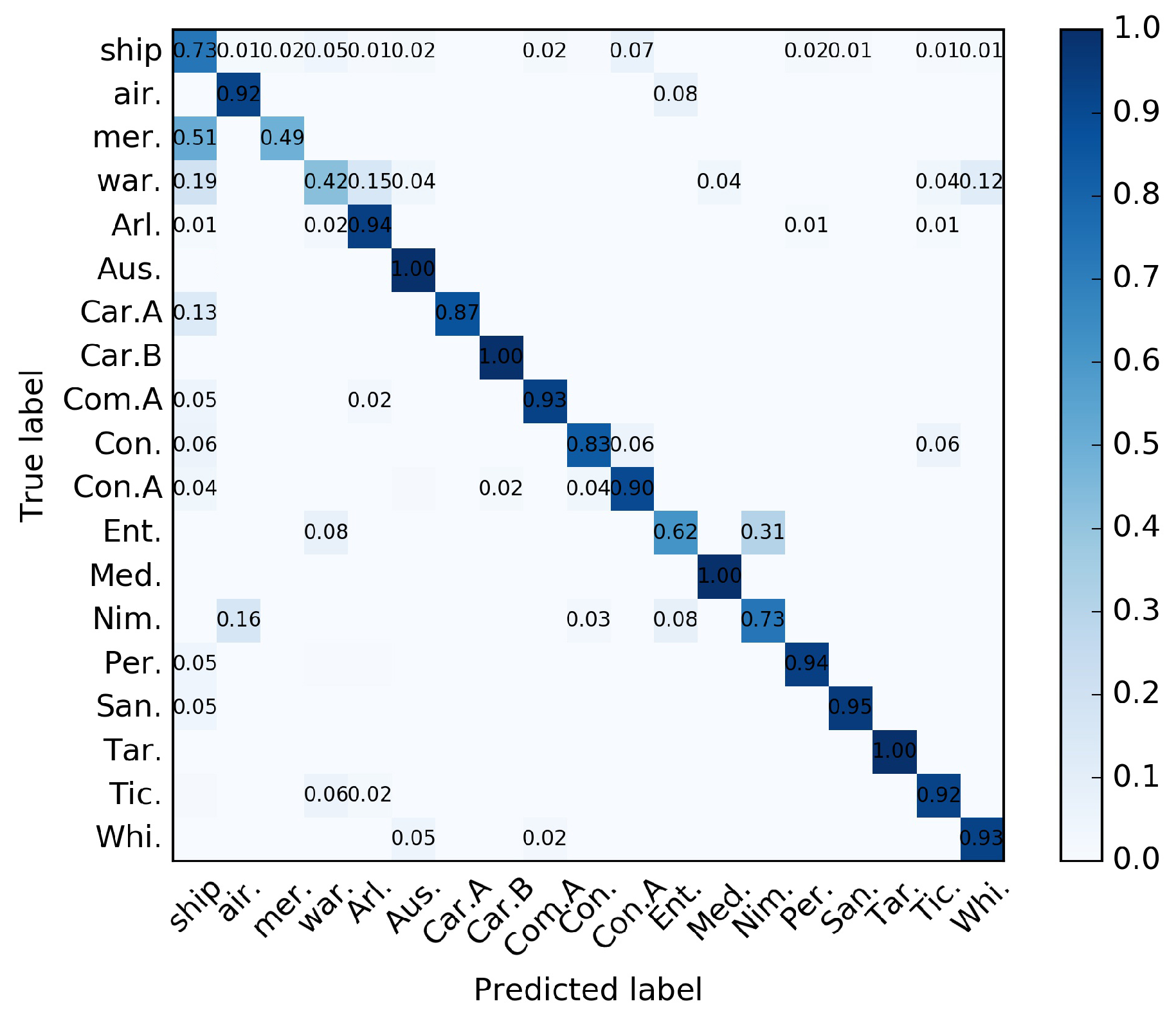
Table 6, we found the results of the classes belonging to L2 level to be poor, especially for the classes mer. and war. The AP values were only obtained 17.9% and 11.5%, respectively. Besides, we found that the accuracy of class Nim. was worse than other methods.
The confusion matrix was analyzed, of which the classes of the L2 level were easy to confuse and classified into other classes, as shown in 
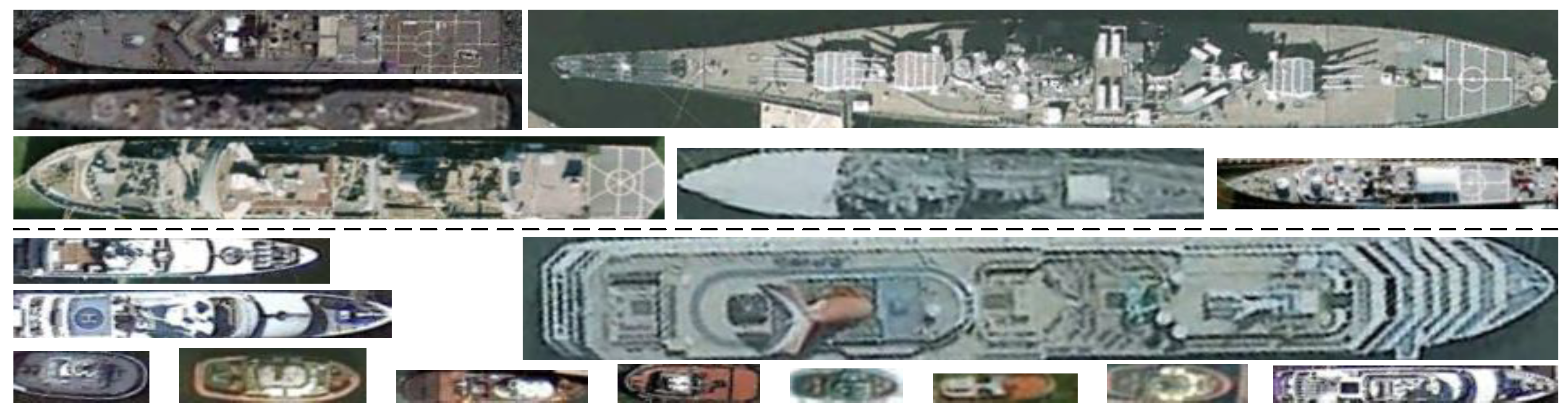
Figure 13. These classes consisted of different types of ships, making intra-class variance larger and inter-class variance decrease. As shown in Figure 14, we show samples of training image patches obtained from the classes mer. and war. Different from the concrete types belonging to the L3 level, we can see a high diversity in sizes, textures, and colors among these examples belonging to the same class. On the other hand, we observed that some small-sized ships were assigned to the background because they did not have ground-truth labels in the dataset, which also enhanced the severity of the confusion. We will investigate how to improve the performance of the impure categories as described above in our future work.
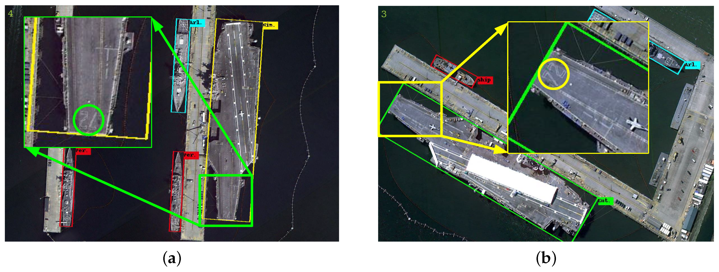
As for the problem about the Nimitz class, there were two factors contributing to this situation. One was the small inter-class variance and the inaccuracies of the ground-truth data. As shown in Figure 15, there were no obvious differences between the classes air., Ent. and Nim.. In addition, we noticed the inaccuracies of the ground-truth data, such as those shown in Figure 16. Obviously, the correct label of the aircraft carrier in Figure 16b is Nim. Therefore, the PSG augmentation strategy may exacerbate this problem and lead to performance degradation. The confusion matrix in 
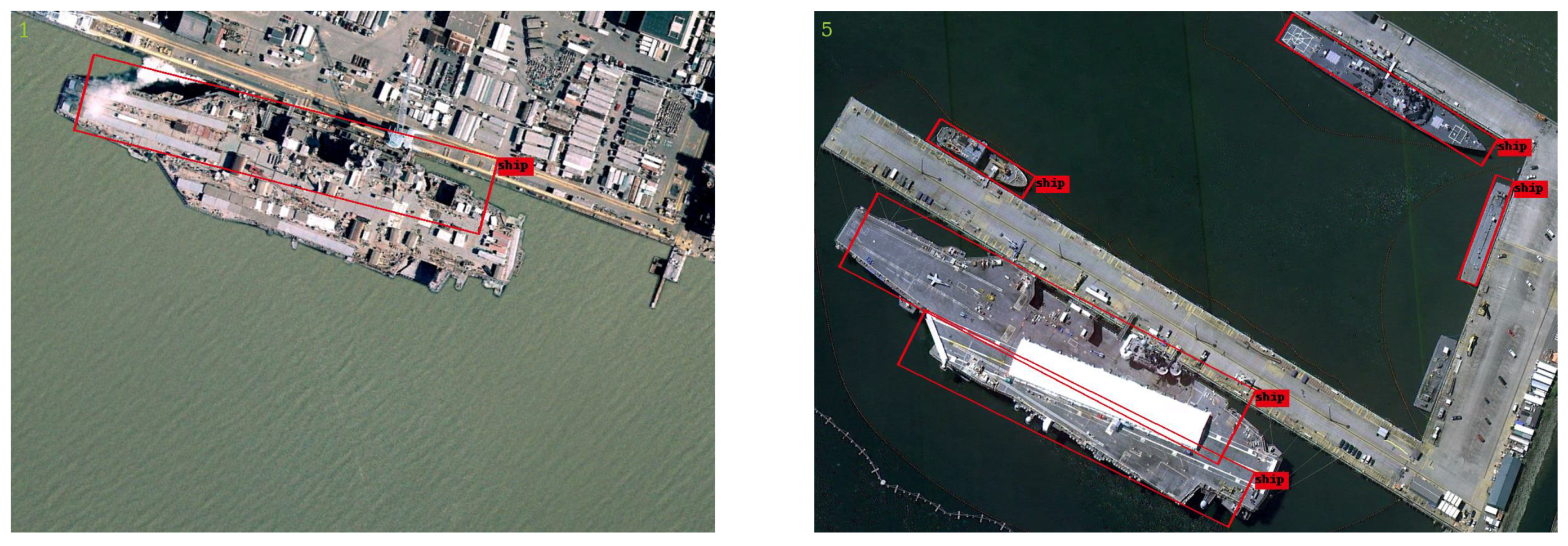
Figure 13 could show a similar conclusion as well. The other was that the detection results of aircraft carrier targets were not ideal. As shown in Figure 17, the rotated bounding box only contained part of the aircraft carrier targets, and even one target had two incomplete detection results. The reasons for the unsatisfactory examples will be investigated in our future work.
Although there are already many ship remote sensing datasets, there is a lack of specific category information for ships. Most of them only labeled categories as coarse-grained or even ignored categories. Furthermore, the ship number in different types has an unbalanced distribution. Therefore, because of the scarcity of training samples and the class imbalance, the improvement of its performance has been deeply influenced. In the future, while accumulating ship samples, we will carry out more detailed labeling of the ships.

5. Conclusions

In this paper, we proposed the rotation-based ship detection and category recognition framework, which consisted of two phases: the location phase and the classification phase. A rotation-based network with an SLC module and HRoI pooling layer was built to produce accurate rotated bounding boxes and achieve a higher recall rate. The ship category classification network was used to classify ships from different subcategories. The STC operation was introduced to connect the two phases and align the discriminative regions. A PSG was used to simulate the output style of the ship detector during the training process, which can address the problem of insufficient samples and class imbalance. In future work, we will try to explore how to train our framework together with the ship detector and classification in an end-to-end manner.

Author Contributions

Formal analysis, Y.F.; funding acquisition, W.D. and X.S.; investigation, Y.F.; methodology, Y.F.; supervision, W.D., X.S., M.Y., and X.G.; visualization, Y.F.; writing, original draft, Y.F.; writing, review and editing, Y.F., W.D., X.S., M.Y., and X.G.

Funding

This work was supported by the National Natural Science Foundation of China (NSFC) under Grant No. 41701508.

Acknowledgments

The authors would like to thank all the colleagues in the lab who generously provided their original images and helped to annotate the images. The authors are very grateful to the anonymous reviewers for their helpful suggestions.

Conflicts of Interest

The authors declare no conflict of interest.

Appendix A. Materials and Implementation Details

In this section, we will describe all materials used and the implementation details of our methods. We used a workstation with 32 GB RAM, an Intel Core i7-6700k processor, and one NVIDIA GeForce GTX 1080 GPU card under CUDA 8.0 and CuDNN 6.0. Our methods, using the Python language, were implemented based on the publicly available Keras [53] framework.
For the location phase, we added the rotation proposals on the ResNet-101-based [53] Faster R-CNN [21] and introduced the FPN [38] structure to combine the different semantic features. The above network initialized by the pretraining model for MS COCO [54] was used as our baseline. We adopted the image-centric sampling strategy [45]. Due to the large difference of the image sizes, we used an input size of 1025 × 1025 to reduce the distortion of the input images. Each mini-batch had one image, and each image had 256 sample RRoIs [38], with a ratio of 1:2 of positives to negatives [21,38,45]. Due to the dataset not being very large, we trained the network for 60 epochs with a small starting learning rate of 3e-4, which was decreased by 10 at Epoch 42 and Epoch 54, respectively. We used a common setting for weight decay with 0.001 and momentum with 0.9. We set the output score threshold to 0.1 in order to keep more detection results. Other parameters not mentioned followed the setting of Faster R-CNN [21].
As for the classification phase, we calculated the IoU value between the ground-truth box and the patch obtain from the STC operation and then assigned the patch the same category label as the ground-truth box with IoU > 0.5. Other patches were set as the background. For a fair comparison, we used the same backbone (ResNet-50 in this paper) for the different classification networks. In additional, except for the PSG, we did not use other augmentation technologies like color, contrast, sharpness, etc.

References

  1. Iervolino, P.; Guida, R. A novel ship detector based on the generalized-likelihood ratio test for SAR imagery. IEEE J. Sel. Top. Appl. Earth Obs. Remote Sens. 2017, 10, 3616–3630. [Google Scholar] [CrossRef]
  2. De Maio, A.; Orlando, D.; Pallotta, L.; Clemente, C. A multifamily GLRT for oil spill detection. IEEE Trans. Geosci. Remote Sens. 2016, 55, 63–79. [Google Scholar] [CrossRef]
  3. Deng, B.; Wang, H.Q.; Li, X.; Qin, Y.L.; Wang, J.T. Generalised likelihood ratio test detector for micro-motion targets in synthetic aperture radar raw signals. IET Radar Sonar Navig. 2011, 5, 528–535. [Google Scholar] [CrossRef]
  4. Iervolino, P.; Guida, R.; Whittaker, P. A new GLRT-based ship detection technique in SAR images. In Proceedings of the IEEE International Geoscience and Remote Sensing Symposium 2015 (IGARSS), Milan, Italy, 26–31 July 2015; pp. 3131–3134. [Google Scholar]
  5. Graziano, M.; D’Errico, M.; Rufino, G. Wake component detection in X-band SAR images for ship heading and velocity estimation. Remote Sens. 2016, 8, 498. [Google Scholar] [CrossRef]
  6. Graziano, M.; Grasso, M.; D’Errico, M. Performance analysis of ship wake detection on Sentinel-1 SAR images. Remote Sens. 2017, 9, 1107. [Google Scholar] [CrossRef]
  7. Biondi, F. Low rank plus sparse decomposition of synthetic aperture radar data for maritime surveillance. In Proceedings of the 2016 4th International Workshop on Compressed Sensing Theory and Its Applications to Radar, Sonar and Remote Sensing (CoSeRa), Aachen, Germany, 19–22 September 2016; pp. 75–79. [Google Scholar]
  8. Biondi, F. Low-rank plus sparse decomposition and localized radon transform for ship-wake detection in synthetic aperture radar images. IEEE Geosci. Remote Sens. Lett. 2017, 15, 117–121. [Google Scholar] [CrossRef]
  9. Biondi, F. A polarimetric extension of low-rank plus sparse decomposition and radon transform for ship wake detection in synthetic aperture radar images. IEEE Geosci. Remote Sens. Lett. 2018, 16, 75–79. [Google Scholar] [CrossRef]
  10. Filippo, B. COSMO-SkyMed staring spotlight SAR data for micro-motion and inclination angle estimation of ships by pixel tracking and convex optimization. Remote Sens. 2019, 11, 766. [Google Scholar] [CrossRef]
  11. Krizhevsky, A.; Sutskever, I.; Hinton, G.E. Imagenet classification with deep convolutional neural networks. In Proceedings of the Advances in Neural Information Processing Systems, Lake Tahoe, NV, USA, 3–9 December 2012; pp. 1097–1105. [Google Scholar]
  12. Zou, Z.; Shi, Z. Ship detection in spaceborne optical image with SVD networks. IEEE Trans. Geosci. Remote Sens. 2016, 54, 5832–5845. [Google Scholar] [CrossRef]
  13. Li, Q.; Mou, L.; Liu, Q.; Wang, Y.; Xiao, X.Z. HSF-net: Multiscale deep feature embedding for ship detection in optical remote sensing imagery. IEEE Trans. Geosci. Remote Sens. 2018, 56, 1–15. [Google Scholar] [CrossRef]
  14. Huang, G.; Wan, Z.; Liu, X.; Hui, J.; Wang, Z.; Zhang, Z. Ship detection based on squeeze excitation skip-connection path networks for optical remote sensing images. Neurocomputing 2019, 332, 215–223. [Google Scholar] [CrossRef]
  15. Li, K.; Cheng, G.; Bu, S.; You, X. Rotation-insensitive and context-augmented object detection in remote sensing images. IEEE Trans. Geosci. Remote Sens. 2018, 56, 2337–2348. [Google Scholar] [CrossRef]
  16. Yao, Y.; Jiang, Z.; Zhang, H.; Zhao, D.; Cai, B. Ship detection in optical remote sensing images based on deep convolutional neural networks. J. Appl. Remote Sens. 2017, 11, 042611. [Google Scholar] [CrossRef]
  17. Liu, Z.; Hu, J.; Weng, L.; Yang, Y. Rotated region based CNN for ship detection. In Proceedings of the IEEE International Conference on Image Processing, Athens, Greece, 7–10 October 2018. [Google Scholar]
  18. Zhang, Z.; Guo, W.; Zhu, S.; Yu, W. Toward arbitrary-oriented ship detection with rotated region proposal and discrimination networks. IEEE Geosci. Remote Sens. Lett. 2018, 15, 1745–1749. [Google Scholar] [CrossRef]
  19. Yang, X.; Sun, H.; Fu, K.; Yang, J.; Sun, X.; Yan, M.; Guo, Z. Automatic ship detection in remote sensing images from google earth of complex scenes based on multiscale rotation dense feature pyramid networks. Remote Sens. 2018, 10, 132. [Google Scholar] [CrossRef]
  20. Fu, K.; Li, Y.; Sun, H.; Yang, X.; Xu, G.; Li, Y.; Sun, X. A ship rotation detection model in remote sensing images based on feature fusion pyramid network and deep reinforcement learning. Remote Sens. 2018, 10, 1922. [Google Scholar] [CrossRef]
  21. Ren, S.; He, K.; Girshick, R.; Sun, J. Faster r-cnn: Towards real-time object detection with region proposal networks. In Proceedings of the Advances in Neural Information Processing Systems, Montreal, QC, Canada, 7–12 December 2015; pp. 91–99. [Google Scholar]
  22. Ma, J.; Shao, W.; Ye, H.; Wang, L.; Wang, H.; Zheng, Y.; Xue, X. Arbitrary-oriented scene text detection via rotation proposals. IEEE Trans. Multimed. 2018, 20, 3111–3122. [Google Scholar] [CrossRef]
  23. He, K.; Gkioxari, G.; Dollar, P.; Girshick, R.B. Mask R-CNN. In Proceedings of the International Conference on Computer Cision, Venice, Italy, 22–29 October 2017; pp. 2980–2988. [Google Scholar]
  24. Hong, Z.; Tian, X.; Chao, W.; Fan, W.; Bo, Z. Merchant vessel classification based on scattering component analysis for COSMO-SkyMed SAR images. IEEE Geosci. Remote Sens. Lett. 2013, 10, 1275–1279. [Google Scholar]
  25. Xing, X.; Ji, K.; Zou, H.; Chen, W.; Sun, J. Ship classification in TerraSAR-X images with feature space based sparse representation. IEEE Geosci. Remote Sens. Lett. 2013, 10, 1562–1566. [Google Scholar] [CrossRef]
  26. Wu, J.; Zhu, Y.; Wang, Z.; Song, Z.; Liu, X.; Wang, W.; Zhang, Z.; Yu, Y.; Xu, Z.; Zhang, T.; et al. A novel ship classification approach for high resolution SAR images based on the BDA-KELM classification model. Int. J. Remote Sens. 2017, 38, 6457–6476. [Google Scholar] [CrossRef]
  27. Oliveau, Q.; Sahbi, H. Learning attribute representations for remote sensing ship category classification. IEEE J. Sel. Top. Appl. Earth Obs. Remote Sens. 2017, 10, 2830–2840. [Google Scholar] [CrossRef]
  28. Simonyan, K.; Zisserman, A. Very deep convolutional networks for large-scale image recognition. In Proceedings of the International Conference on Learning Representations, San Diego, CA, USA, 7–9 May 2015. [Google Scholar]
  29. Szegedy, C.; Liu, W.; Jia, Y.; Sermanet, P.; Reed, S.; Anguelov, D.; Erhan, D.; Vanhoucke, V.; Rabinovich, A. Going deeper with convolutions. In Proceedings of the IEEE Conference on Computer Vision and Pattern Recognition, Boston, MA, USA, 7–12 June 2015; pp. 1–9. [Google Scholar]
  30. Huang, G.; Liu, Z.; Der Maaten, L.V.; Weinberger, K.Q. Densely connected convolutional networks. In Proceedings of the IEEE Conference on Computer Vision and Pattern Recognition, Honolulu, HI, USA, 21–26 July 2017; pp. 2261–2269. [Google Scholar]
  31. Bentes, C.; Velotto, D.; Tings, B. Ship classification in terrasar-x images with convolutional neural networks. IEEE J. Ocean. Eng. 2018, 43, 258–266. [Google Scholar] [CrossRef]
  32. Ma, M.; Chen, J.; Liu, W.; Yang, W. Ship classification and detection based on CNN using GF-3 SAR images. Remote Sens. 2018, 10, 2043. [Google Scholar] [CrossRef]
  33. Krishna, R.; Zhu, Y.; Groth, O.; Johnson, J.; Hata, K.; Kravitz, J.; Chen, S.; Kalantidis, Y.; Li, L.J.; Shamma, D.A. Visual genome: Connecting language and vision using crowdsourced dense image annotations. Int. J. Comput. Vis. 2016, 123, 32–73. [Google Scholar] [CrossRef]
  34. Chen, Z.; Gao, X. An Improved Algorithm for Ship Target Detection in SAR Images Based on Faster R-CNN. In Proceedings of the Ninth International Conference on Intelligent Control and Information Processing (ICICIP 2018), Wanzhou, China, 9–11 November 2018; pp. 39–43. [Google Scholar]
  35. Li, S.; Zhang, Z.; Li, B.; Li, C. Multiscale rotated bounding box-based deep learning method for detecting ship targets in remote sensing images. Sensors 2018, 18, 2702. [Google Scholar] [CrossRef]
  36. Koo, J.; Seo, J.; Jeon, S.; Choe, J.; Jeon, T. RBox-CNN: Rotated bounding box based CNN for ship detection in remote sensing image. In Proceedings of the 26th ACM SIGSPATIAL International Conference on Advances in Geographic Information Systems (ACM 2018), Seattle, WA, USA, 6–9 November 2018; pp. 420–423. [Google Scholar]
  37. Liao, M.; Zhu, Z.; Shi, B.; Xia, G.s.; Bai, X. Rotation-sensitive regression for oriented scene text detection. In Proceedings of the IEEE Conference on Computer Vision and Pattern Recognition, Salt Lake City, UT, USA, 18–22 June 2018; pp. 5909–5918. [Google Scholar]
  38. Lin, T.Y.; Dollár, P.; Girshick, R.; He, K.; Hariharan, B.; Belongie, S. Feature pyramid networks for object detection. In Proceedings of the IEEE Conference on Computer Vision and Pattern Recognition, Honolulu, HI, USA, 21–26 July 2017; pp. 2117–2125. [Google Scholar]
  39. Lin, T.Y.; Goyal, P.; Girshick, R.; He, K.; Dollár, P. Focal loss for dense object detection. In Proceedings of the IEEE Conference on Computer Vision and Pattern Recognition, Honolulu, HI, USA, 21–26 July 2017; pp. 2980–2988. [Google Scholar]
  40. Girshick, R.B.; Donahue, J.; Darrell, T.; Malik, J. Rich feature hierarchies for accurate object detection and semantic segmentation. In Proceedings of the IEEE Conference on Computer Vision and Pattern Recognition, Columbus, OH, USA, 24–27 Jun 2014; pp. 580–587. [Google Scholar]
  41. Plaisted, D.A.; Hong, J. A heuristic triangulation algorithm. J. Algorithm. 1987, 8, 405–437. [Google Scholar] [CrossRef]
  42. Liu, Z.; Wang, H.; Weng, L.; Yang, Y. Ship rotated bounding box space for ship extraction from high-resolution optical satellite images with complex backgrounds. IEEE Geosci. Remote Sens. Lett. 2016, 13, 1074–1078. [Google Scholar] [CrossRef]
  43. Xia, G.S.; Bai, X.; Ding, J.; Zhu, Z.; Belongie, S.; Luo, J.; Datcu, M.; Pelillo, M.; Zhang, L. DOTA: A large-scale dataset for object detection in aerial images. In Proceedings of the IEEE Conference on Computer Vision and Pattern Recognition, Salt Lake City, UT, USA, 18–22 June 2018; pp. 3974–3983. [Google Scholar]
  44. Cheng, G.; Han, J.; Zhou, P.; Guo, L. Multi-class geospatial object detection and geographic image classification based on collection of part detectors. ISPRS J. Photogramm. Remote Sens. 2014, 98, 119–132. [Google Scholar] [CrossRef]
  45. Girshick, R. Fast R-CNN. In Proceedings of the IEEE International Conference on Computer Vision (ICCV), Santiago, Chile, 7–13 December 2015. [Google Scholar]
  46. Feng, Y.; Diao, W.; Chang, Z.; Yan, M.; Sun, X.; Gao, X. Ship instance segmentation from remote sensing images using sequence local context module. arXiv 2019, arXiv:1904.09823. [Google Scholar]
  47. He, K.; Zhang, X.; Ren, S.; Sun, J. Spatial pyramid pooling in deep convolutional networks for visual recognition. IEEE Trans. Pattern Anal. Machine Intell. 2015, 37, 1904–1916. [Google Scholar] [CrossRef]
  48. Zhao, B.; Feng, J.; Wu, X.; Yan, S. A survey on deep learning-based fine-grained object classification and semantic segmentation. Int. J. Autom. Comput. 2017, 14, 119–135. [Google Scholar] [CrossRef]
  49. Long, J.; Shelhamer, E.; Darrell, T. Fully convolutional networks for semantic segmentation. In Proceedings of the IEEE Conference on Computer Vision and Pattern Recognition, Boston, MA, USA, 7–12 June 2015; pp. 3431–3440. [Google Scholar]
  50. Zhang, X.; Wei, Y.; Feng, J.; Yang, Y.; Huang, T.S. Adversarial complementary learning for weakly supervised object localization. In Proceedings of the IEEE Conference on Computer Vision and Pattern Recognition, Salt Lake City, UT, USA, 18–22 June 2018; pp. 1325–1334. [Google Scholar]
  51. Liu, Z.; Yuan, L.; Weng, L.; Yang, Y. A high resolution optical satellite image dataset for ship recognition and some new baselines. In Proceedings of the 6th International Conference on Pattern Recognition Applications and Methods, Porto, Portugal, 24–26 February 2017; pp. 324–331. [Google Scholar]
  52. Everingham, M.; Van Gool, L.; Williams, C.K.; Winn, J.; Zisserman, A. The pascal visual object classes (voc) challenge. Int. J. Comput. Vis. 2010, 88, 303–338. [Google Scholar] [CrossRef]
  53. He, K.; Zhang, X.; Ren, S.; Sun, J. Deep residual learning for image recognition. In Proceedings of the IEEE Conference on Computer Vision and Pattern Recognition, Las Vegas, NV, USA, 27–30 June 2016; pp. 770–778. [Google Scholar]
  54. Lin, T.; Maire, M.; Belongie, S.J.; Hays, J.; Perona, P.; Ramanan, D.; Dollar, P.; Zitnick, C.L. Microsoft COCO: Common Objects in Context. In Proceedings of the European Conference on Computer Vision, Zurich, Switzerland, 5–12 September 2014; pp. 740–755. [Google Scholar]
Figure 1. (a) The ground-truth labels of rotated bounding boxes. (b) The ground-truth labels of horizontal bounding boxes. (c) The inaccurate prediction labels of rotated bounding boxes. (d) The overlapping rotated bounding boxes.
Remotesensing 11 01901 g001
Figure 2. Overview of our framework including the detection phase and the classification phase. HRoI, Horizontal Region of Interest; PSG, Proposals Simulation Generator; cls, classification; reg, regression.
Remotesensing 11 01901 g002
Figure 3. The pooling layer in the detection phase: (a) Rotation Region of Interest (RRoI) pooling layer. (b) HRoI pooling layer.
Remotesensing 11 01901 g003
Figure 4. The sequence local context module.
Remotesensing 11 01901 g004
Figure 5. The distribution of the image patches on HRSC2016.
Remotesensing 11 01901 g005
Figure 6. Illustration of the three different classification networks.
Remotesensing 11 01901 g006
Figure 7. The Gaussian distributions of the rotated bounding box offsets with x , y , w , h , θ for different classes on HRSC2016.
Remotesensing 11 01901 g007
Figure 8. The box-plot of IoU belonging to TP for different methods.
Remotesensing 11 01901 g008
Figure 9. Detailed analysis of the P-R curves with different IoU thresholds on HRSC2016: (a) the P-R curves of RDFPN; (b) the P-R curves of the baseline; (c) the P-R curves of our detection network.
Remotesensing 11 01901 g009
Figure 10. Comparisons of the inference speed of our framework. Num refers to the number of test images.
Remotesensing 11 01901 g010
Figure 11. The samples of the detection results on HRSC2016. The samples in the first row are generated by the baseline; the ones in the second row are predicted by our detection part SHD; the images in the third and the fourth row are predicted by our whole framework.
Remotesensing 11 01901 g011
Figure 12. The samples of the detection results on the MWC.
Remotesensing 11 01901 g012
Figure 13. The confusion matrix for the ship classification network on HRSC2016.
Remotesensing 11 01901 g013
Figure 14. A sample of the training images from the classes mer. and war. on HRSC2016. Above the dotted line is the class war., and below is the class mer.
Remotesensing 11 01901 g014
Figure 15. The training patches from left to right belong to classes Nim., Ent. and air., respectively.
Remotesensing 11 01901 g015
Figure 16. Examples of ground-truth labeling errors. The aircraft carrier in the two pictures is same: (a) The aircraft carrier with correct label Nim. (b) The aircraft carrier with incorrect label Ent.
Remotesensing 11 01901 g016
Figure 17. Incomplete detection results of aircraft carriers.
Remotesensing 11 01901 g017
Table 1. The information and physical sizes of different classes on the Multiclass Warship Collection (MWC). Chung, ChungHai; For, Formidable; Henry, Henry J Kaiser; Kno, Knox; LaF, La Fayette.
ItemArl.Aus.Chung.End.For.Henry.Kno.LaF.Nim.Per.Tic.
Training set15532837416570458468165107
Testing set449221948171222203932
Length156.5173105141114.8206.7133.6154332135.6173
Width20.432152116.329.714.312.440.813.716.8
Table 2. Classification accuracies (%) of different methods among different targets on HRSC2016. RDFPN, Rotation Dense Feature Pyramid Network; SHD, Sequence Local Context-HRoI Detection; HBB, Horizontal Bounding Box.
MethodShipAir.Mer.War.Arl.Aus.Car.ACar.BCom.ACon.Con.AEnt.Med.Nim.Per.San.Tar.Tic.Whi.OA
RDFPN [19]57.492.324.625.995.197.356.3100.078.683.379.538.590.068.492.595.5100.092.781.076.2
SHD-HBB48.369.25.329.687.891.956.375.076.277.887.723.1100.084.285.059.182.084.578.669.5
SHD (ours)68.192.324.648.193.9100.062.587.595.283.391.069.2100.086.890.290.998.090.988.181.5
Table 3. Compression of recall and the location metric for different methods on HRSC2016.
Method R 0.5 RL 0.5 R 0.6 RL 0.6 R 0.7 RL 0.7 R 0.8 RL 0.8 R 0.9 RL 0.9
RDFPN [19]0.890.680.830.650.670.540.370.320.050.05
Baseline0.930.700.850.650.630.510.280.240.030.03
SHD (ours)0.970.800.940.770.870.730.630.550.130.12
Table 4. Classification accuracies (%) of different strategies among different targets on HRSC2016.
MethodShipAir.Mer.War.Arl.Aus.Car.ACar.BCom.ACon.Con.AEnt.Med.Nim.Per.San.Tar.Tic.Whi.OA
RoIAlign10.861.523.411.584.194.686.793.892.977.890.153.8100.043.263.495.598.080.785.460.2
FCN31.869.219.150.089.6100.060.087.592.972.286.584.6100.048.677.990.993.961.580.566.0
RoIAlign-f36.761.570.211.590.991.993.387.597.672.289.261.5100.070.388.590.9100.089.078.073.4
FCN-f47.284.683.061.593.397.373.387.592.972.289.253.8100.094.694.786.493.982.675.678.2
Resize66.892.338.338.593.9100.066.787.590.588.987.476.9100.081.190.886.498.090.887.881.6
Table 5. Classification accuracies (%) of augmentation among different targets on HRSC2016.
MethodShipAir.Mer.War.Arl.Aus.Car.ACar.BCom.ACon.Con.AEnt.Med.Nim.Per.San.Tar.Tic.Whi.OA
Random68.992.310.634.693.997.383.696.590.577.887.469.2100.091.991.395.298.090.887.882.1
PSG (ours)73.492.348.942.393.9100.086.7100.092.983.390.161.5100.073.093.995.4100.091.992.784.5
Table 6. The average precision (%) values of all the classes on HRSC2016. SRBBS, Ship Rotated Bounding Boxes Space.
MethodShipAir.Mer.War.Arl.Aus.Car.ACar.BCom.ACon.Con.AEnt.Med.Nim.Per.San.Tar.Tic.Whi.Total
CP [17] (Fast R-CNN [45] + SRBBS)35.318.220.50.855.832.635.961.043.130.350.812.830.132.337.336.531.441.130.833.5
BL2 [17] (CP + RBB)41.941.212.83.971.043.253.167.857.136.849.63.078.844.643.951.450.957.450.945.2
RC1 [17] (BL2 + RRoI)34.353.927.43.965.348.761.067.850.556.262.723.098.559.347.645.562.448.651.851.0
RC2 [17] (RC1 + Multi-NMS)32.940.318.24.861.042.756.757.638.440.256.318.262.565.042.331.567.049.845.843.7
Faster R-CNN [21]45.618.954.46.885.026.372.751.617.042.160.23.00.064.651.80.079.569.420.940.5
RDFPN [19]46.730.822.011.868.926.955.565.033.242.152.143.834.568.049.113.775.066.620.443.5
SHD + RoIAlign6.928.515.44.480.990.772.266.949.961.950.429.484.536.260.077.450.565.274.652.9
SHD + FCN20.445.610.95.887.087.456.383.677.062.553.650.490.848.666.079.684.561.576.660.4
SHD + Resize43.986.721.510.891.583.251.784.684.069.664.563.895.569.687.980.993.185.981.371.1
RDFPN [19] + Resize + PSG36.872.310.033.487.680.570.894.585.258.467.355.390.978.882.995.089.184.275.471.0
SHD-HBB + Resize + PSG30.872.515.010.881.472.865.169.972.236.754.354.695.572.880.268.692.179.278.363.3
SHDRP (SHD + Resize + PSG) (ours)52.377.717.911.591.386.377.798.985.364.772.855.795.567.291.992.496.588.286.374.2
Table 7. The average precision (%) values of all the classes on the MWC.
MethodArl.Aus.Chung.End.For.Henry.Kno.LaF.Nim.Per.Tic.Total
RDFPN [19] + Resize + PSG79.955.694.894.766.836.680.395.280.561.552.172.5
SHDRP (ours)94.362.095.594.792.749.898.796.395.284.194.787.1

