Crop Monitoring Using Sentinel-1 Data: A Case Study from The Netherlands

 ,
,  ,
,
Abstract
1. Introduction
2. Data and Methods
2.1. Study Area
2.2. Hydrometeorological Ground Data
2.3. Ground Data at 24 Parcels
2.4. Sentinel-1 Data
Detecting Emergence, Closure and Harvest Date
3. Results and Discussion
3.1. Hydrometeorological Data
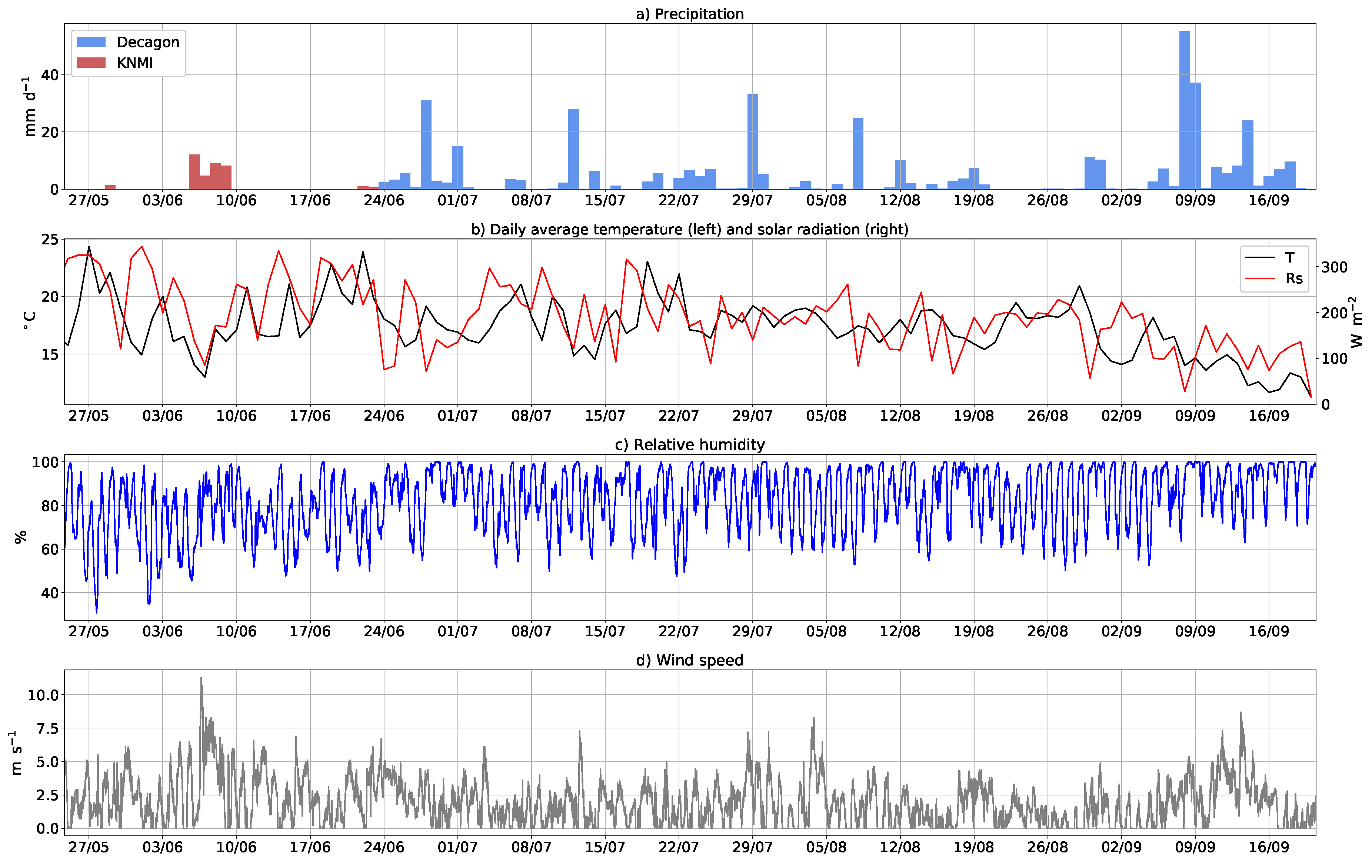
3.1.1. Weather Station Data
3.1.2. Interception and Dew
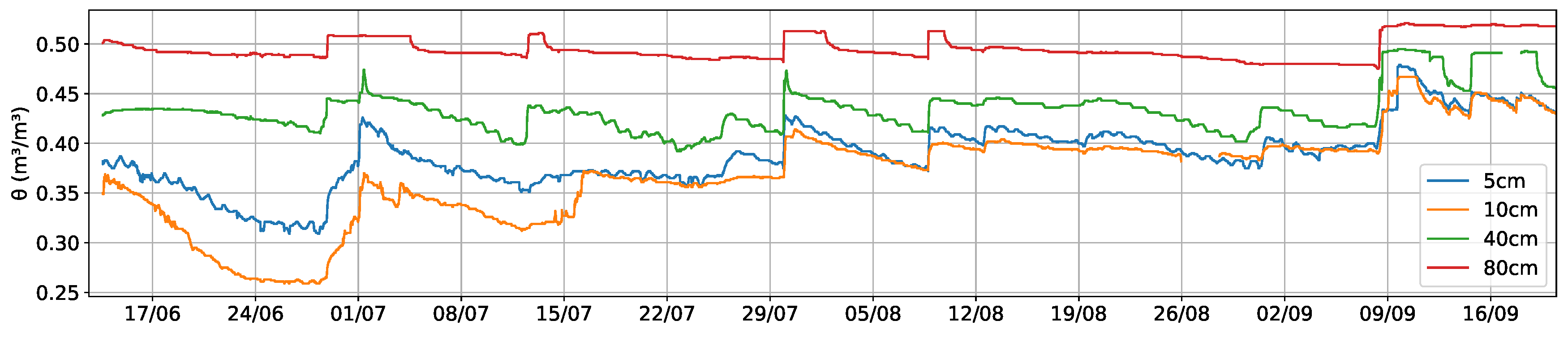
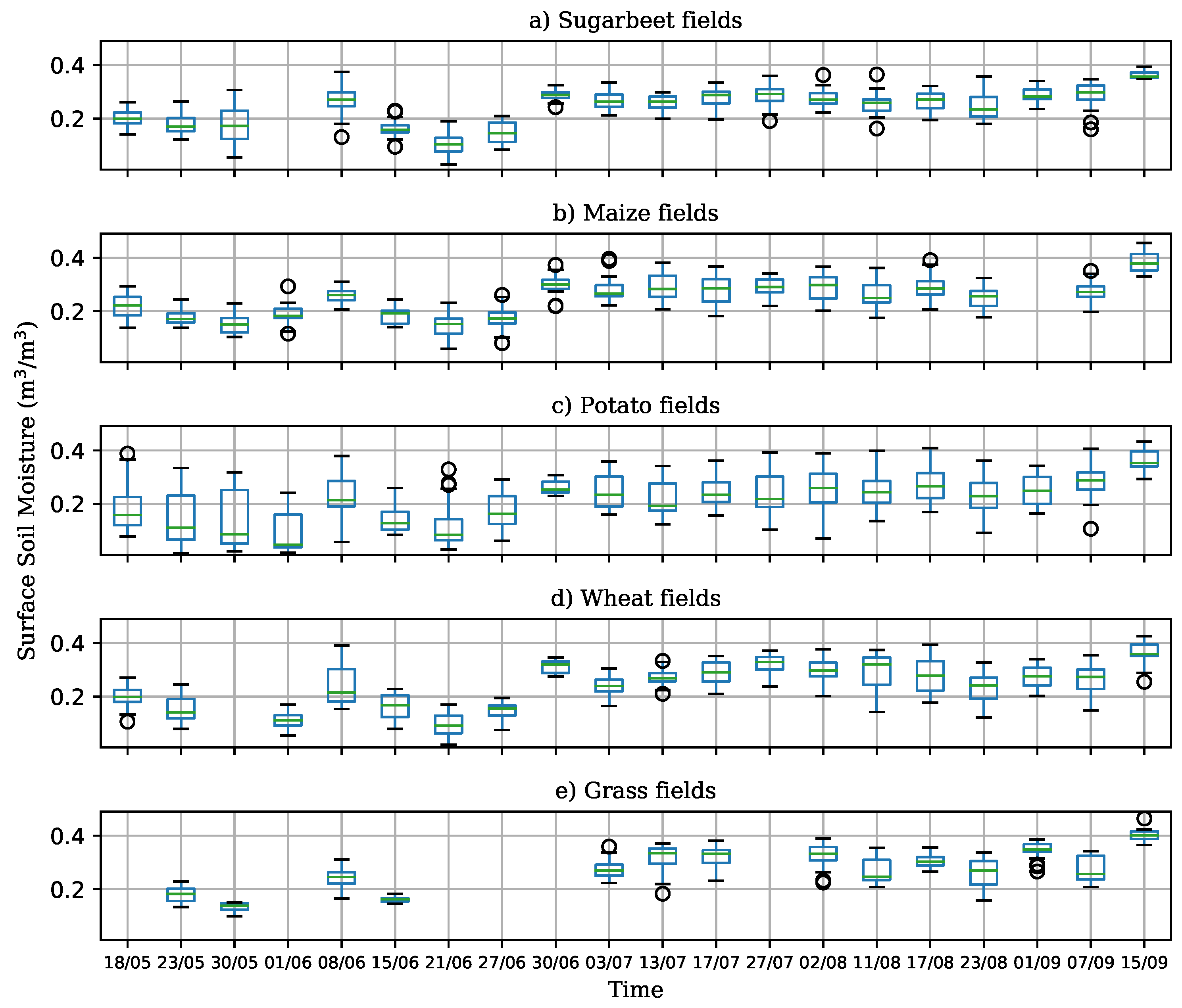
3.1.3. Soil Moisture
3.2. Sentinel-1 Time Series
3.2.1. Maize
3.2.2. Potato
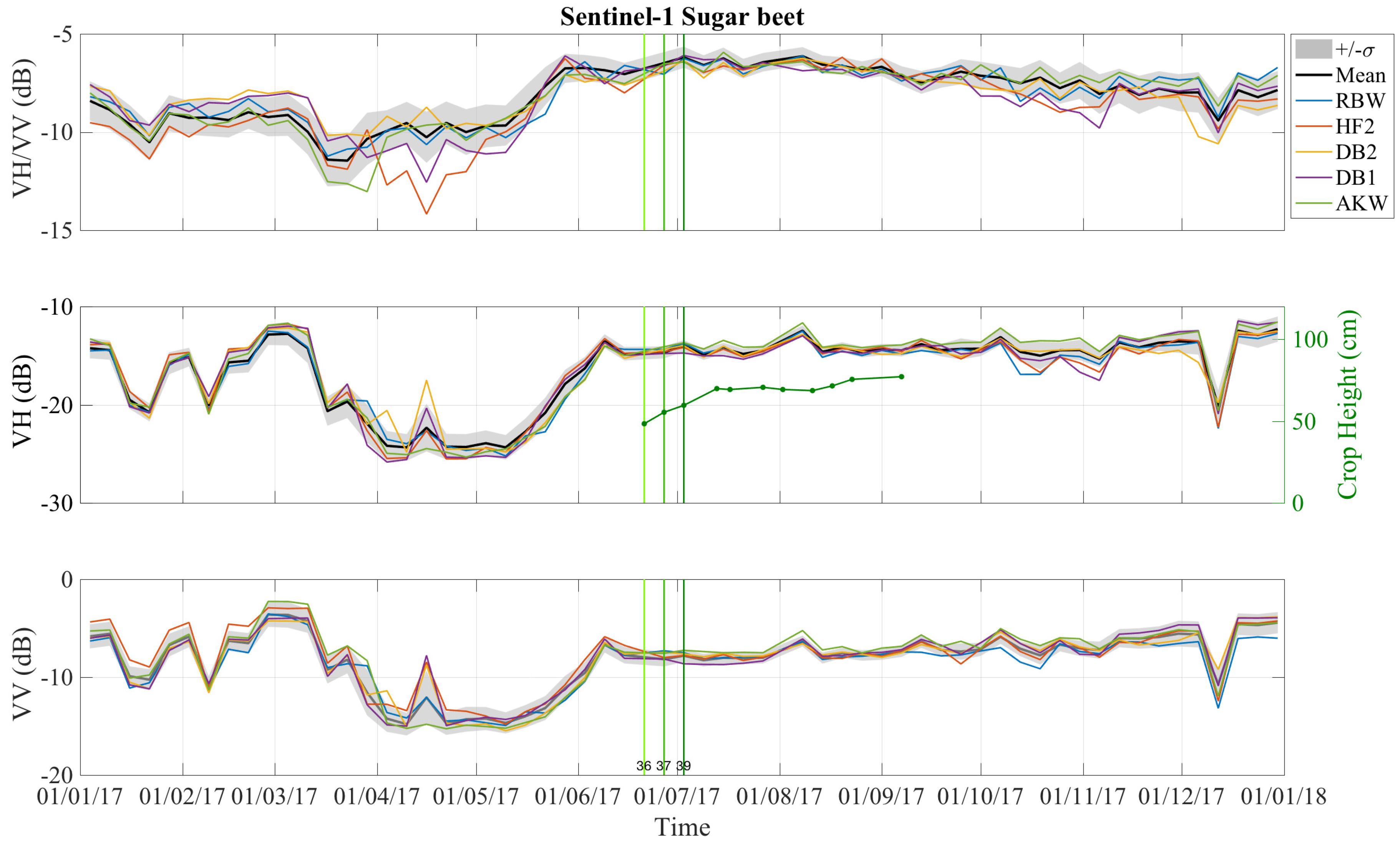
3.2.3. Sugar Beet
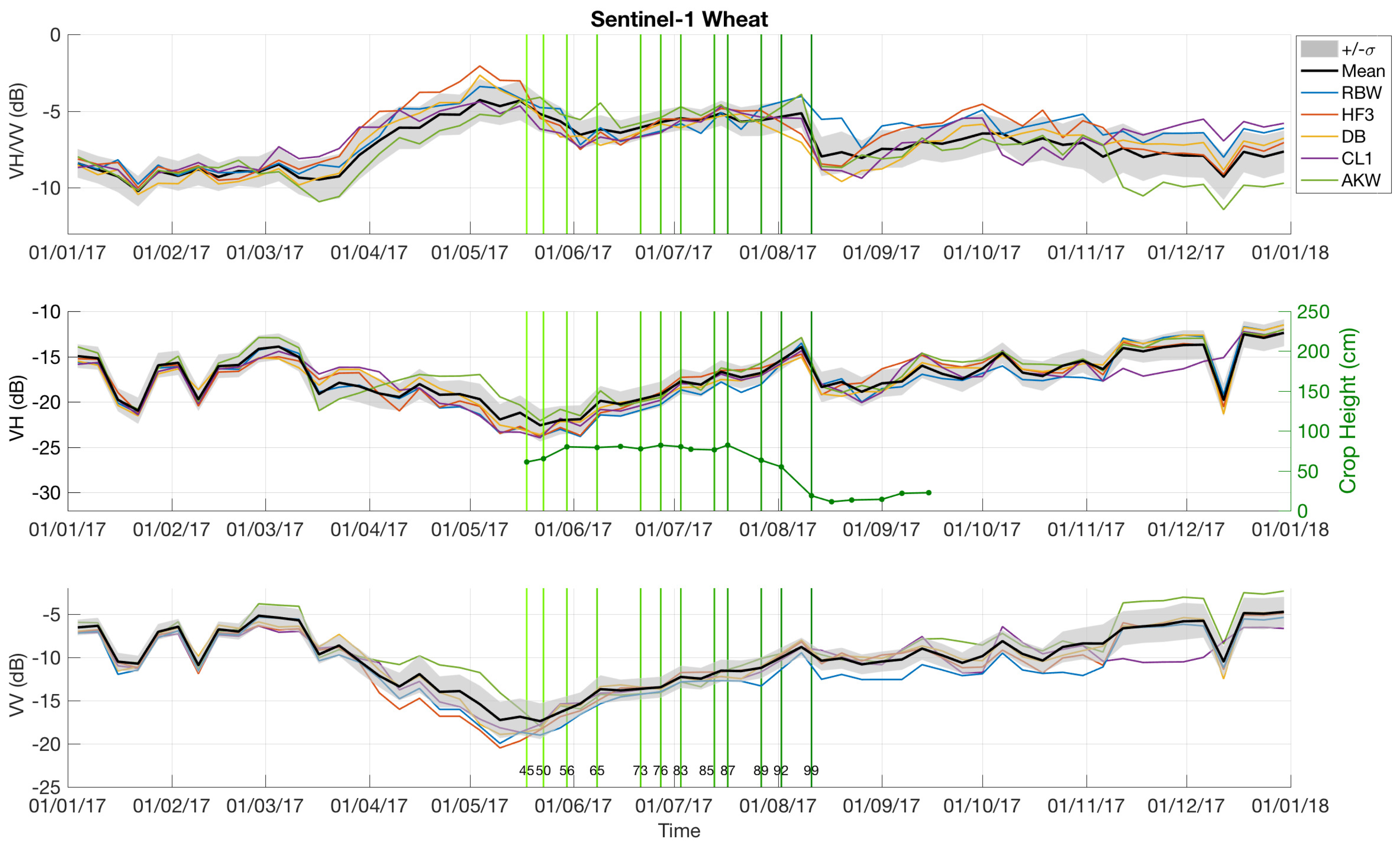
3.2.4. Winter Wheat
3.2.5. English Rye Grass
3.3. Mapping Key Dates
3.3.1. Emergence Date
3.3.2. Closure Date
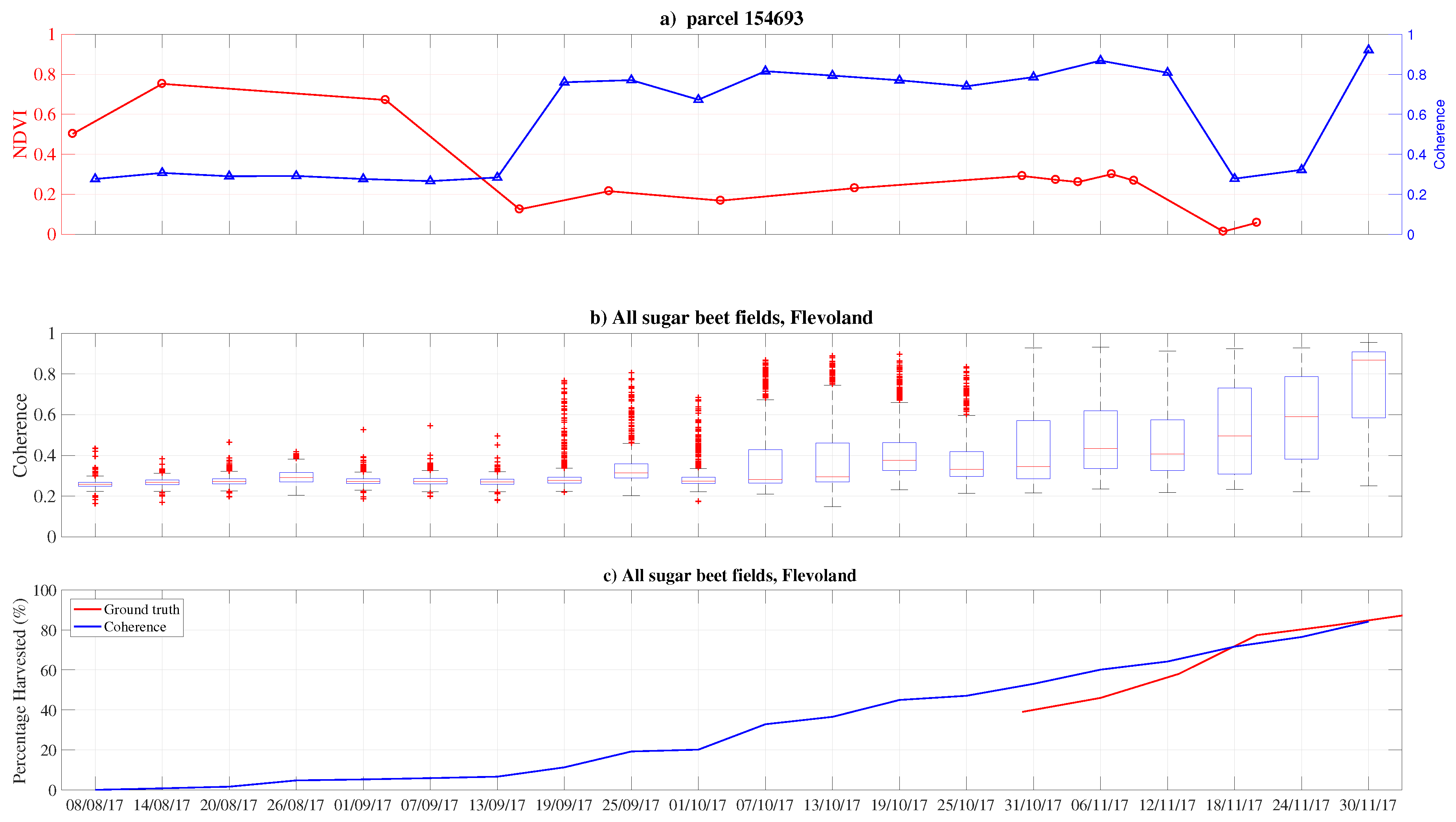
3.3.3. Sugar Beet Harvest Date
3.3.4. Potato Haulming and Harvest Date
4. Conclusions
Supplementary Materials
Author Contributions
Funding
Acknowledgments
Conflicts of Interest
References
- Berkhout, P. Agricultural Economic Report 2015 Summary; SUMMARY Report 2015-092; Agricultural Economics Research Institute (LEI): The Hague, The Netherlands, 2015. [Google Scholar]
- The Netherlands in 2030; Technical Report; ECORYS: Rotterdam, The Netherlands, 2014.
- Brisco, B.; Brown, R.; Hirose, T.; McNairn, H.; Staenz, K. Precision Agriculture and the Role of Remote Sensing: A Review. Can. J. Remote Sens. 1998, 24, 315–327. [Google Scholar] [CrossRef]
- Mulla, D.J. Twenty five years of remote sensing in precision agriculture: Key advances and remaining knowledge gaps. Biosyst. Eng. 2013, 114, 358–371. [Google Scholar] [CrossRef]
- Kross, A.; McNairn, H.; Lapen, D.; Sunohara, M.; Champagne, C. Assessment of RapidEye vegetation indices for estimation of leaf area index and biomass in corn and soybean crops. Int. J. Appl. Earth Obs. Geoinf. 2015, 34, 235–248. [Google Scholar] [CrossRef]
- Georgi, C.; Spengler, D.; Itzerott, S.; Kleinschmit, B. Automatic delineation algorithm for site-specific management zones based on satellite remote sensing data. Precis. Agric. 2018, 19, 684–707. [Google Scholar] [CrossRef]
- Vizzari, M.; Santaga, F.; Benincasa, P. Sentinel 2-Based Nitrogen VRT Fertilization in Wheat: Comparison between Traditional and Simple Precision Practices. Agronomy 2019, 9, 278. [Google Scholar] [CrossRef]
- Houborg, R.; McCabe, M.F. Daily Retrieval of NDVI and LAI at 3 m Resolution via the Fusion of CubeSat, Landsat, and MODIS Data. Remote Sens. 2018, 10, 890. [Google Scholar] [CrossRef]
- Pilot4CAP—European Commission. 2018. Available online: https://g4cap.jrc.ec.europa.eu/g4cap/Default.aspx?tabid=354 (accessed on 5 July 2019).
- Satellietdataportaal.nl V1. Available online: https://satellietdataportaal.nl/ (accessed on 5 July 2019).
- Van der Wal, T.; Abma, B.; Viguria, A.; Prévinaire, E.; Zarco-Tejada, P.J.; Serruys, P.; van Valkengoed, E.; van der Voet, P. Fieldcopter: Unmanned Aerial Systems for Crop Monitoring Services. In Precision Agriculture’13; Stafford, J.V., Ed.; Wageningen Academic Publishers: Wageningen, The Netherlands, 2013; pp. 169–175. [Google Scholar]
- Bush, T.F.; Ulaby, F.T. An evaluation of radar as a crop classifier. Remote Sens. Environ. 1978, 7, 15–36. [Google Scholar] [CrossRef]
- Ulaby, F.; Bush, T.; Batlivala, P. Radar response to vegetation II: 8-18 GHz band. IEEE Trans. Antennas Propag. 1975, 23, 608–618. [Google Scholar] [CrossRef]
- Ulaby, F. Radar response to vegetation. IEEE Trans. Antennas Propag. 1975, 23, 36–45. [Google Scholar] [CrossRef]
- Wang, J.R.; Engman, E.T.; Mo, T.; Schmugge, T.J.; Shiue, J.C. The Effects of Soil Moisture, Surface Roughness, and Vegetation on L-Band Emission and Backscatter. IEEE Trans. Geosci. Remote Sens. 1987, GE-25, 825–833. [Google Scholar] [CrossRef]
- Bouman, B.A.M.; van Kasteren, H.W.J. Ground-based X-band (3-cm wave) radar backscattering of agricultural crops. I. Sugar beet and potato; backscattering and crop growth. Remote Sens. Environ. 1990, 34, 93–105. [Google Scholar] [CrossRef]
- Steele-Dunne, S.C.; McNairn, H.; Monsivais-Huertero, A.; Judge, J.; Liu, P.W.; Papathanassiou, K. Radar Remote Sensing of Agricultural Canopies: A Review. IEEE J. Sel. Top. Appl. Earth Obs. Remote Sens. 2017, 10, 2249–2273. [Google Scholar] [CrossRef]
- Torres, R.; Snoeij, P.; Geudtner, D.; Bibby, D.; Davidson, M.; Attema, E.; Potin, P.; Rommen, B.; Floury, N.; Brown, M.; et al. GMES Sentinel-1 mission. Remote Sens. Environ. 2012, 120, 9–24. [Google Scholar] [CrossRef]
- Arias, M.; Campo-Bescós, M.A.; Álvarez Mozos, J. Crop Type Mapping Based on Sentinel-1 Backscatter Time Series. In Proceedings of the IGARSS 2018-2018 IEEE International Geoscience and Remote Sensing Symposium, Valencia, Spain, 22–27 July 2018; pp. 6623–6626. [Google Scholar] [CrossRef]
- Kussul, N.; Lavreniuk, M.; Skakun, S.; Shelestov, A. Deep Learning Classification of Land Cover and Crop Types Using Remote Sensing Data. IEEE Geosci. Remote Sens. Lett. 2017, 14, 778–782. [Google Scholar] [CrossRef]
- Torbick, N.; Chowdhury, D.; Salas, W.; Qi, J. Monitoring Rice Agriculture across Myanmar Using Time Series Sentinel-1 Assisted by Landsat-8 and PALSAR-2. Remote Sens. 2017, 9, 119. [Google Scholar] [CrossRef]
- Bazzi, H.; Baghdadi, N.; El Hajj, M.; Zribi, M.; Minh, D.H.T.; Ndikumana, E.; Courault, D.; Belhouchette, H. Mapping Paddy Rice Using Sentinel-1 SAR Time Series in Camargue, France. Remote Sens. 2019, 11, 887. [Google Scholar] [CrossRef]
- Ndikumana, E.; Ho Tong Minh, D.; Baghdadi, N.; Courault, D.; Hossard, L. Deep Recurrent Neural Network for Agricultural Classification using multitemporal SAR Sentinel-1 for Camargue, France. Remote Sens. 2018, 10, 1217. [Google Scholar] [CrossRef]
- Veloso, A.; Mermoz, S.; Bouvet, A.; Le Toan, T.; Planells, M.; Dejoux, J.F.; Ceschia, E. Understanding the temporal behavior of crops using Sentinel-1 and Sentinel-2-like data for agricultural applications. Remote Sens. Environ. 2017, 199, 415–426. [Google Scholar] [CrossRef]
- Vreugdenhil, M.; Wagner, W.; Bauer-Marschallinger, B.; Pfeil, I.; Teubner, I.; Rüdiger, C.; Strauss, P. Sensitivity of Sentinel-1 Backscatter to Vegetation Dynamics: An Austrian Case Study. Remote Sens. 2018, 10, 1396. [Google Scholar] [CrossRef]
- Introductie—PDOK. Available online: https://www.pdok.nl/introductie/-/article/basisregistratie-gewaspercelen-brp- (accessed on 5 July 2019).
- Haagsma, M. Crop Monitoring with Radar. Master’s Thesis, TUDelft, Delft, The Netherlands, 2015. [Google Scholar]
- KNMI—Daggegevens van het weer in Nederland. Available online: https://knmi.nl/nederland-nu/klimatologie/daggegevens (accessed on 5 July 2019).
- Gillespie, T.; Brisco, B.; Brown, R.; Sofko, G. Radar detection of a dew event in wheat. Remote Sens. Environ. 1990, 33, 151–156. [Google Scholar] [CrossRef]
- Herold, M.; Pathe, C.; Schmullius, C.C. The effect of free vegetation water on the multi-frequency and polarimetric radar backscatter—First, results from the TerraDew 2000 campaign. In IGARSS 2001. Scanning the Present and Resolving the Future. Proceedings of the IEEE 2001 International Geoscience and Remote Sensing Symposium (Cat. No. 01CH37217), Sydney, NSW, Australia, 9–13 July 2001; IEEE: Piscataway, NJ, USA, 2001; Volume 5, pp. 2445–2447. [Google Scholar] [CrossRef]
- Wood, D.; McNairn, H.; Brown, R.J.; Dixon, R. The effect of dew on the use of RADARSAT-1 for crop monitoring: Choosing between ascending and descending orbits. Remote Sens. Environ. 2002, 80, 241–247. [Google Scholar] [CrossRef]
- Russell, E.S. Effect of Dew and Intercepted Precipitation on Radar Backscatter of a Soybean Canopy. Master’s Thesis, Iowa State University, Ames, IA, USA, 2011. [Google Scholar]
- Riedel, T.; Pathe, C.; Thiel, C.; Herold, M.; Schmullius, C. Systematic Investigation on the Effect of Dew and Interception on Multifrequency and Multipolarimetric RADAR Backscatter Signals. In Proceedings of the Third International Symposium on Retrieval of Bio- and Geophysical Parameters from SAR Data for Land Applications, Sheffield, UK, 11–14 September 2002; pp. 99–104. [Google Scholar]
- Soil-Specific Calibrations for METER Soil Moisture Sensors | METER Environment. Available online: https://www.metergroup.com/environment/articles/how-calibrate-soil-moisture-sensors/ (accessed on 5 July 2019).
- ML3 ThetaProbe Soil Moisture Sensor—Soil Moisture Measurement—Soil Moisture Meter. Available online: https://www.delta-t.co.uk/product/ml3/ (accessed on 5 July 2019).
- Meier, U. Growth Stages of Mono-and Dicotyledonous Plants; Blackwell Wissenschafts-Verlag: Hoboken, NJ, USA, 1997; p. 158. [Google Scholar]
- Meier, W.; Bleiholder, H.; Buhr, L.; Feller, C.; Hack, H.; Heß, M.; Lancashire, P.D.; Schnock, U.; Stauß, R.; Van den Boom, T.; et al. The BBCH System to Coding the Phenological Growth Stages of Plants—History and Publications. J. Kult. 2009, 61, 41–52. [Google Scholar]
- Gorelick, N.; Hancher, M.; Dixon, M.; Ilyushchenko, S.; Thau, D.; Moore, R. Google Earth Engine: Planetary-scale geospatial analysis for everyone. Remote Sens. Environ. 2017. [Google Scholar] [CrossRef]
- Copernicus Open Access Hub. Available online: https://scihub.copernicus.eu/ (accessed on 5 July 2019).
- Sentinel-1 Algorithms | Google Earth Engine API. Available online: https://developers.google.com/earth-engine/sentinel1 (accessed on 5 July 2019).
- SNAP—ESA Sentinel Application Platform v6.0.0, Download | STEP. 2018. Available online: https://step.esa.int/main/download/snap-download/ (accessed on 5 July 2019).
- SNAP Documentation | STEP. Available online: https://step.esa.int/main/doc/ (accessed on 5 July 2019).
- 7.2 Opbrengstprognose | Teelthandleiding | Stichting IRS. Available online: https://www.irs.nl/alle/teelthandleiding/7.2-opbrengstprognose (accessed on 5 July 2019).
- Van Swaaij, N. Groei en Ontwikkeling van de Suikerbiet. 2011. Available online: https://www.irs.nl/userfiles/testhandleiding_render/7.1-groei-en-ontwikkeling-van-de-suikerbiet.pdf (accessed on 5 July 2019).
- Bronswijk, J.; Evers-Vermeer, J. Krimpkarakteristieken van Kleigronden In Nederland; Technical Report 22; Instituut Voor Cultuurtechniek En Waterhuishoudung (Icw): Wageningen, The Netherlands, 1987. [Google Scholar]
- Baghdadi, N.; Bazzi, H.; El Hajj, M.; Zribi, M. Detection of Frozen Soil Using Sentinel-1 SAR Data. Remote Sens. 2018, 10, 1182. [Google Scholar] [CrossRef]
- Liu, C.; Shang, J.; Vachon, P.W.; McNairn, H. Multiyear Crop Monitoring Using Polarimetric RADARSAT-2 Data. IEEE Trans. Geosci. Remote Sens. 2013, 51, 2227–2240. [Google Scholar] [CrossRef]
- Wiseman, G.; McNairn, H.; Homayouni, S.; Shang, J. RADARSAT-2 Polarimetric SAR Response to Crop Biomass for Agricultural Production Monitoring. IEEE J. Sel. Topics Appl. Earth Obs. Remote Sens. 2014, 7, 4461–4471. [Google Scholar] [CrossRef]
- Moran, M.S.; Alonso, L.; Moreno, J.F.; Mateo, M.P.C. A RADARSAT-2 Quad-Polarized Time Series for Monitoring Crop and Soil Conditions in Barrax, Spain. IEEE Trans. Geosci. Remote Sens. 2012, 50, 14. [Google Scholar] [CrossRef]
- McNairn, H.; Duguay, C.; Brisco, B.; Pultz, T.J. The effect of soil and crop residue characteristics on polarimetric radar response. Remote Sens. Environ. 2002, 80, 308–320. [Google Scholar] [CrossRef]
- Jiao, X.; McNairn, H.; Shang, J.; Pattey, E.; Liu, J.; Champagne, C. The sensitivity of RADARSAT-2 polarimetric SAR data to corn and soybean leaf area index. Can. J. Remote Sens. 2011, 37, 14. [Google Scholar] [CrossRef]
- Ferrazzoli, P.; Paloscia, S.; Pampaloni, P.; Schiavon, G.; Solimini, D.; Coppo, P. Sensitivity of microwave measurements to vegetation biomass and soil moisture content: a case study. IEEE Trans. Geosci. Remote Sens. 1992, 30, 750–756. [Google Scholar] [CrossRef]
- Daughtry, C.S.T.; Ranson, K.J.; Biehl, L.L. C-band backscattering from corn canopies. Int. J. Remote Sens. 1991, 12, 1097–1109. [Google Scholar] [CrossRef]
- Wegmüller, U.; Santoro, M.; Mattia, F.; Balenzano, A.; Satalino, G.; Marzahn, P.; Fischer, G.; Ludwig, R.; Floury, N. Progress in the understanding of narrow directional microwave scattering of agricultural fields. Remote Sens. Environ. 2011, 115, 2423–2433. [Google Scholar] [CrossRef]
- Brown, S.C.; Quegan, S.; Morrison, K.; Bennett, J.C.; Cookmartin, G. High-resolution measurements of scattering in wheat canopies-Implications for crop parameter retrieval. IEEE Trans. Geosci. Remote Sens. 2003, 41, 1602–1610. [Google Scholar] [CrossRef]
- Mattia, F.; Toan, T.L.; Picard, G.; Posa, F.I.; D’Alessio, A.; Notarnicola, C.; Gatti, A.M.; Rinaldi, M.; Satalino, G.; Pasquariello, G. Multitemporal C-band radar measurements on wheat fields. IEEE Trans. Geosci. Remote Sens. 2003, 41, 10. [Google Scholar] [CrossRef]
- Macelloni, G.; Paloscia, S.; Pampaloni, P.; Marliani, F.; Gai, M. The relationship between the backscattering coefficient and the biomass of narrow and broad leaf crops. IEEE Trans. Geosci. Remote Sens. 2001, 39, 873–884. [Google Scholar] [CrossRef]
- Larrañaga, A.; Álvarez Mozos, J.; Albizua, L.; Peters, J. Backscattering Behavior of Rain-Fed Crops Along the Growing Season. IEEE Geosci. Remote Sens. Lett. 2013, 10, 5. [Google Scholar] [CrossRef]
- Picard, G.; Toan, T.L.; Mattia, F. Understanding C-band radar backscatter from wheat canopy using a multiple-scattering coherent model. IEEE Trans. Geosci. Remote Sens. 2003, 41, 1583–1591. [Google Scholar] [CrossRef]


| Relative Orbit | Pass | Local Time | Min. Inc. Angle (°) | Max. Inc. Angle (°) |
|---|---|---|---|---|
| 37 | DESC | 06:49 | 38.9 | 41.9 |
| 161 | ASC | 18.32 | 44.7 | 46.1 |
| 88 | ASC | 18:24 | 36.6 | 40.4 |
| 15 | ASC | 18:15 | 30.0 | 31.5 |
| 110 | DESC | 06:58 | 30.0 | 33.7 |
| Crop Type | Number of Parcels |
|---|---|
| Maize | 335 |
| Potato | 886 |
| Sugar beet | 763 |
| Wheat | 1048 |
| English Rye Grass | 1286 |
| Sensor | A.M. (%) | P.M. (%) |
|---|---|---|
| upper | 45.6 | 19.1 |
| middle | 26.1 | 8.0 |
| lower | 35.2 | 11.4 |
© 2019 by the authors. Licensee MDPI, Basel, Switzerland. This article is an open access article distributed under the terms and conditions of the Creative Commons Attribution (CC BY) license (http://creativecommons.org/licenses/by/4.0/).
Share and Cite
Khabbazan, S.; Vermunt, P.; Steele-Dunne, S.; Ratering Arntz, L.; Marinetti, C.; van der Valk, D.; Iannini, L.; Molijn, R.; Westerdijk, K.; van der Sande, C. Crop Monitoring Using Sentinel-1 Data: A Case Study from The Netherlands. Remote Sens. 2019, 11, 1887. https://doi.org/10.3390/rs11161887
Khabbazan S, Vermunt P, Steele-Dunne S, Ratering Arntz L, Marinetti C, van der Valk D, Iannini L, Molijn R, Westerdijk K, van der Sande C. Crop Monitoring Using Sentinel-1 Data: A Case Study from The Netherlands. Remote Sensing. 2019; 11(16):1887. https://doi.org/10.3390/rs11161887
Chicago/Turabian StyleKhabbazan, Saeed, Paul Vermunt, Susan Steele-Dunne, Lexy Ratering Arntz, Caterina Marinetti, Dirk van der Valk, Lorenzo Iannini, Ramses Molijn, Kees Westerdijk, and Corné van der Sande. 2019. "Crop Monitoring Using Sentinel-1 Data: A Case Study from The Netherlands" Remote Sensing 11, no. 16: 1887. https://doi.org/10.3390/rs11161887
APA StyleKhabbazan, S., Vermunt, P., Steele-Dunne, S., Ratering Arntz, L., Marinetti, C., van der Valk, D., Iannini, L., Molijn, R., Westerdijk, K., & van der Sande, C. (2019). Crop Monitoring Using Sentinel-1 Data: A Case Study from The Netherlands. Remote Sensing, 11(16), 1887. https://doi.org/10.3390/rs11161887