Temporal Evolution of Corn Mass Production Based on Agro-Meteorological Modelling Controlled by Satellite Optical and SAR Images

 , , ,
, , ,
Abstract

1. Introduction
2. Materials and Method
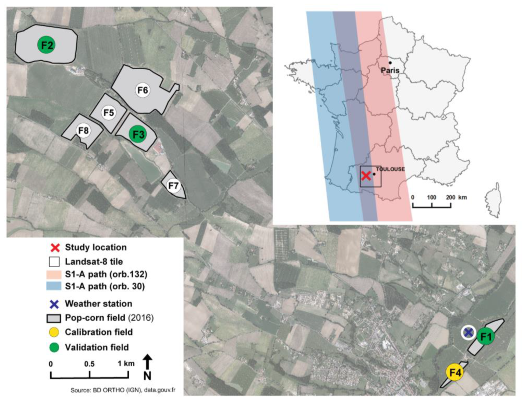
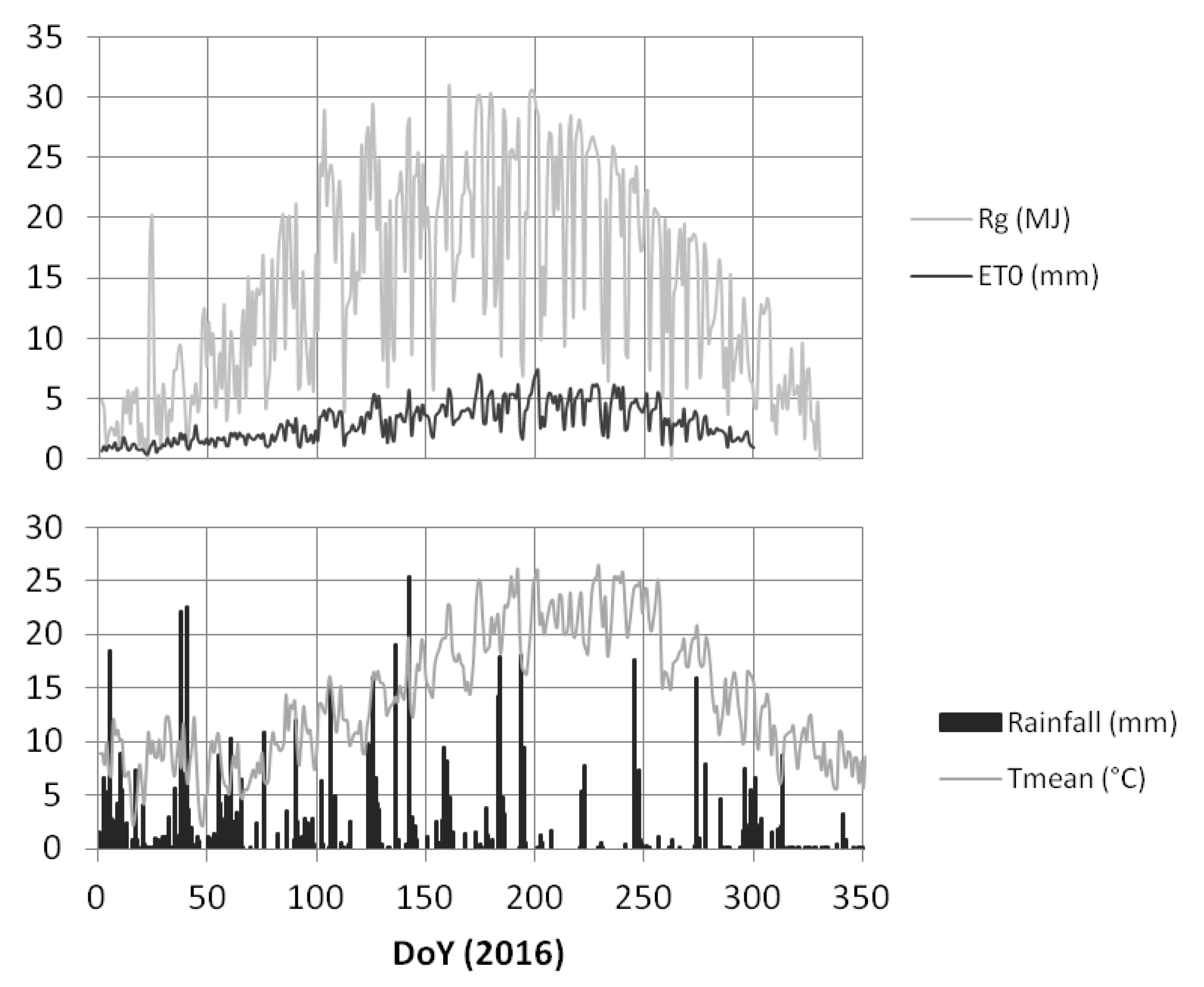
2.1. Site Description
2.2. Satellite and Ground Data
2.2.1. Satellite Data
Acquisition Calendar
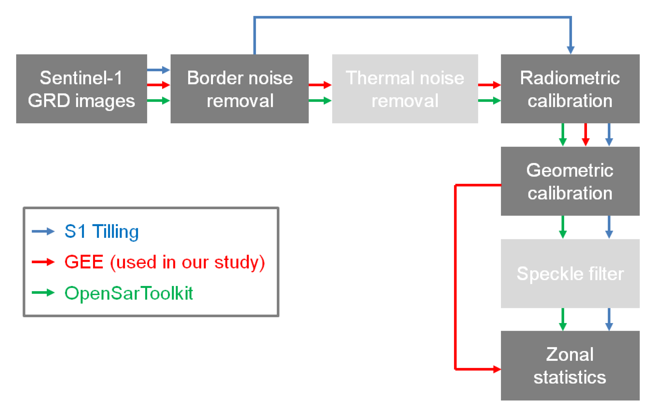
Data Pre-Processing
2.2.2. Ground Data
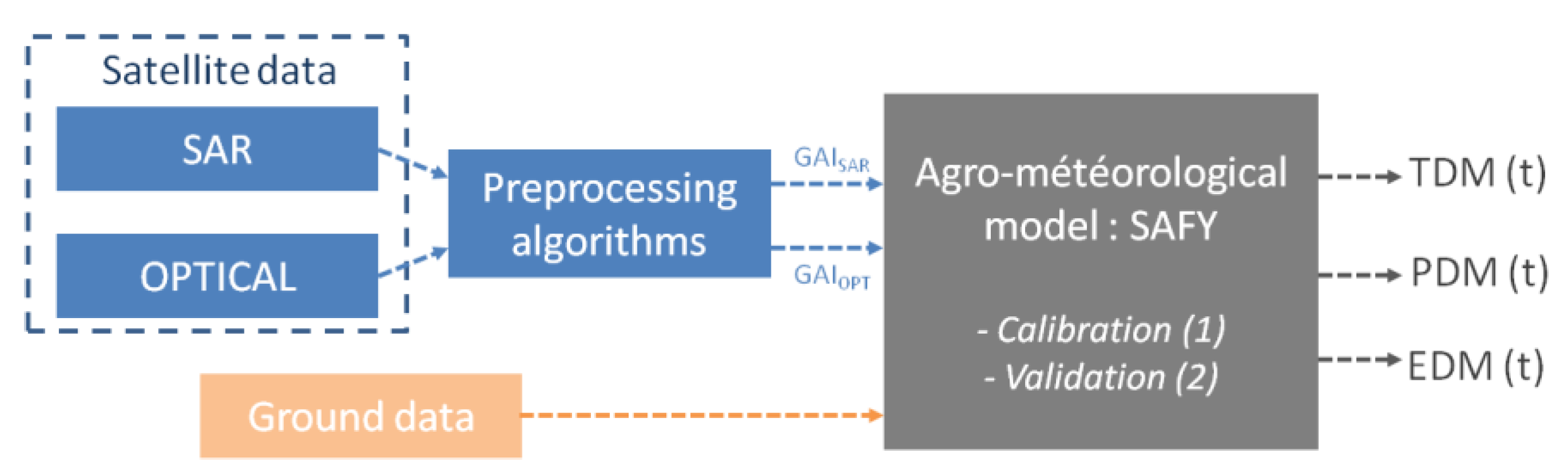
2.3. The Agro-Meteorological Model
2.4. Methodology
3. Results
3.1. Model Calibration
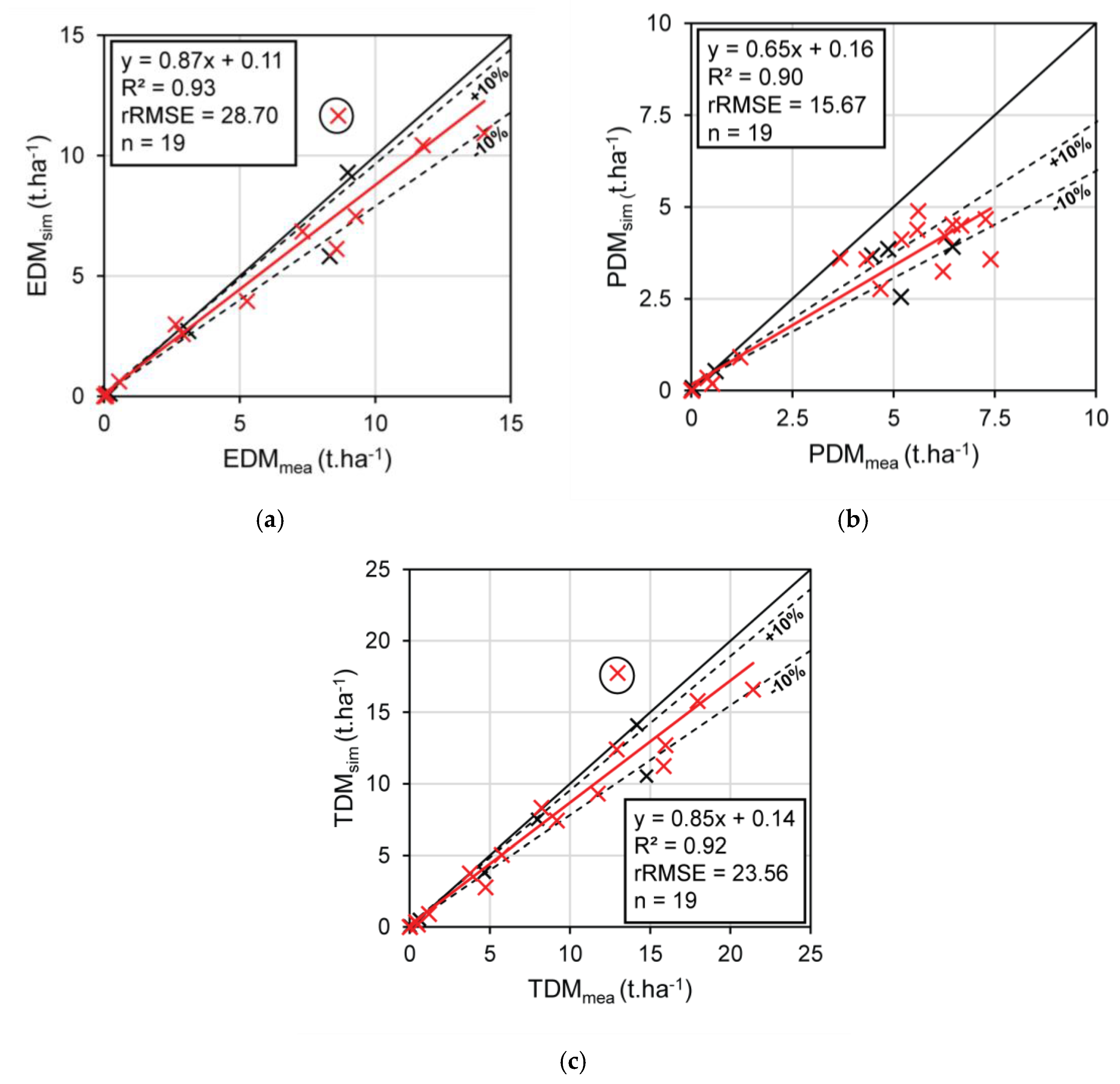
3.2. Model Validation—Mass Retrieval
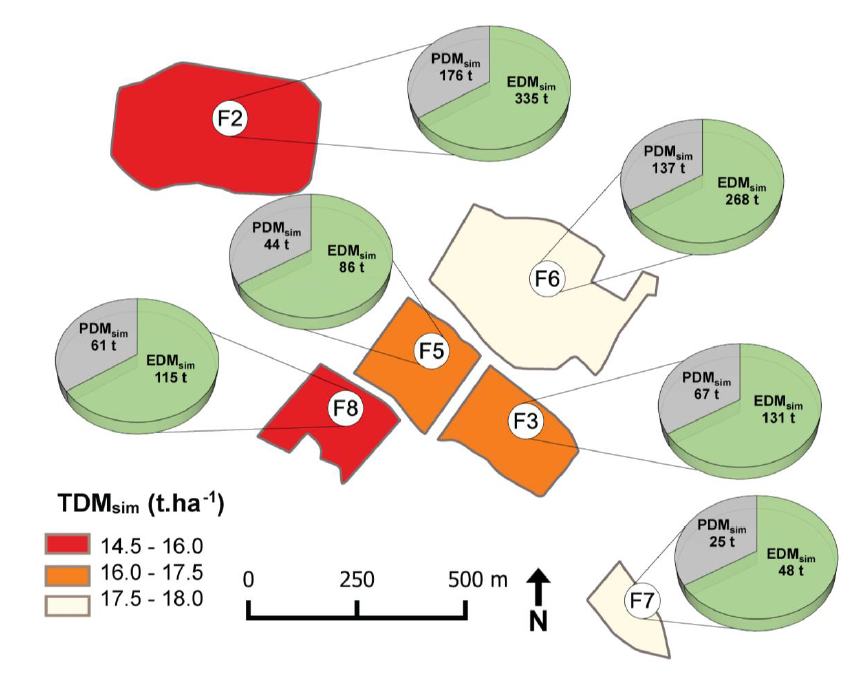
3.3. Mapping the Production of Corn over One Working Farm
4. Discussion
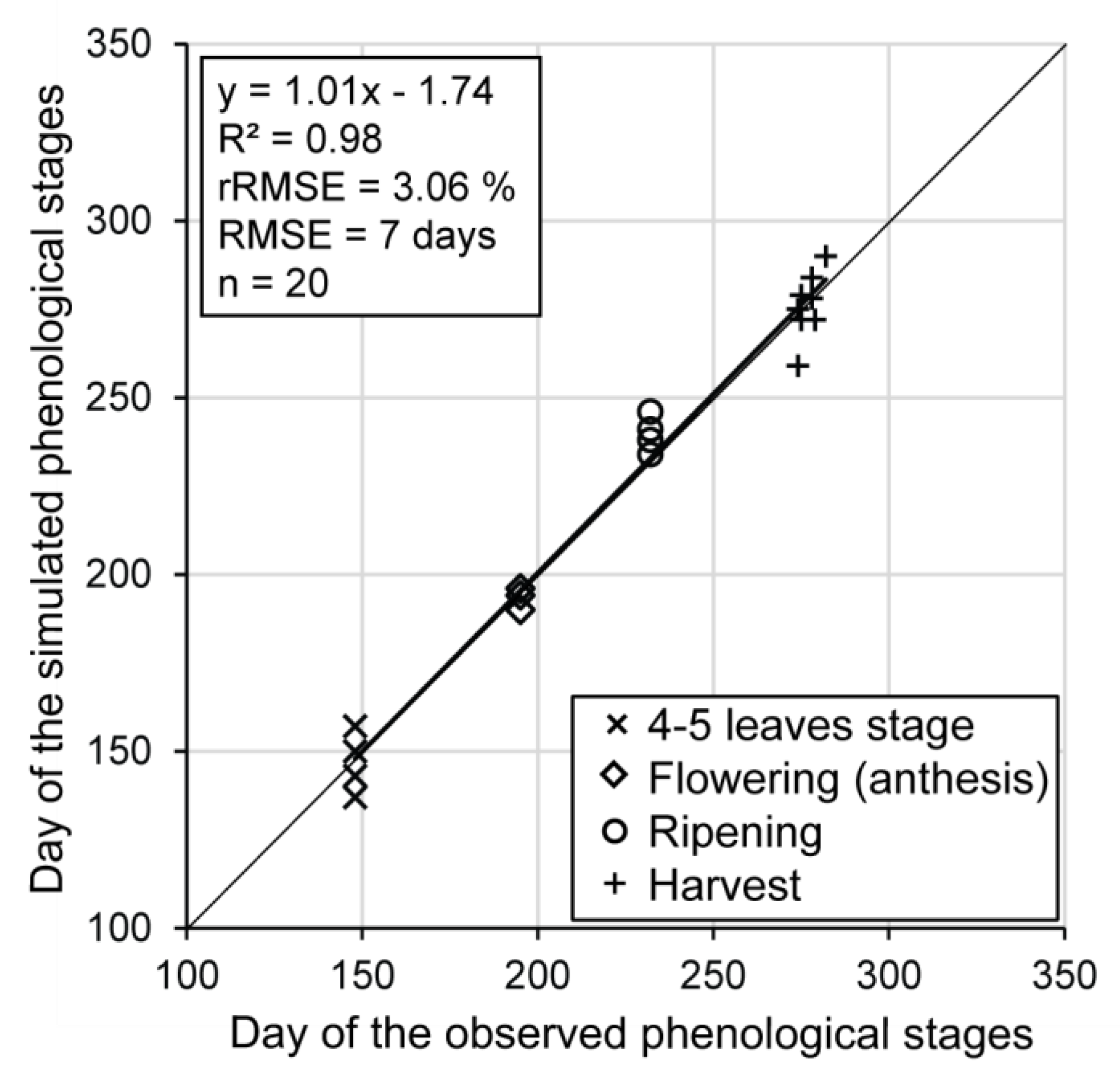
4.1. Can Corn Phenological Stages Be Accurately Inferred?
4.2. Can Vegetation Mass Be Retrieved Irrespective the Phenologic Stage?
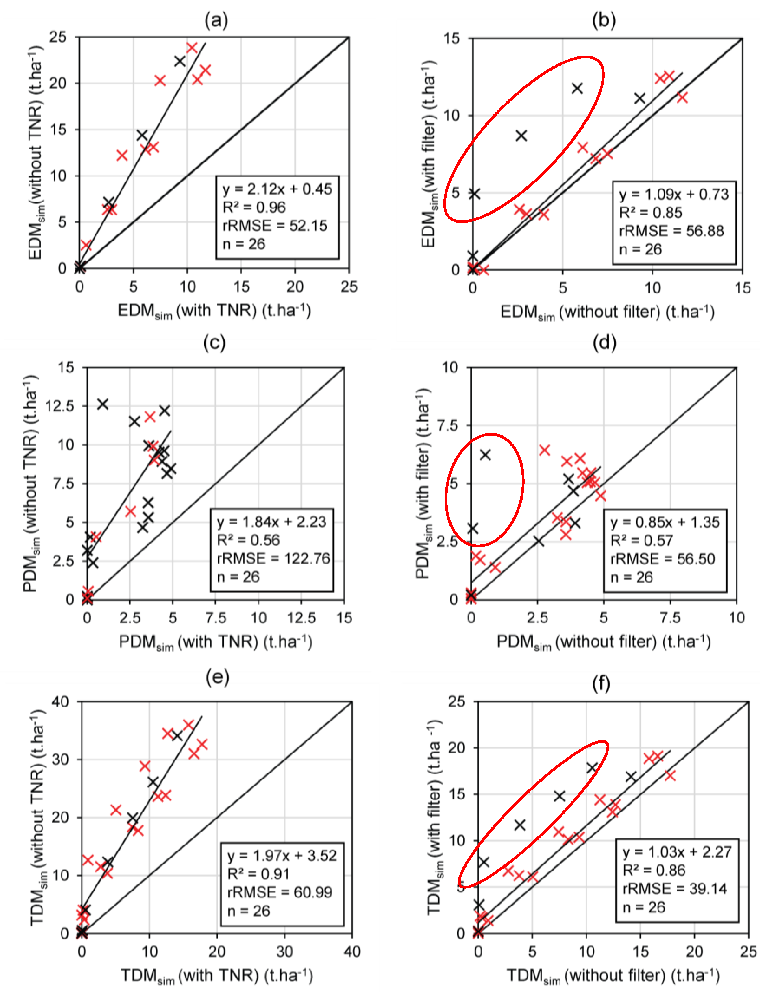
4.3. What Is the Impact of the SAR Preprocessing Algorithm?
4.3.1. Impact of the Speckle Filter on the Backscattering Coefficient at the Field Scale
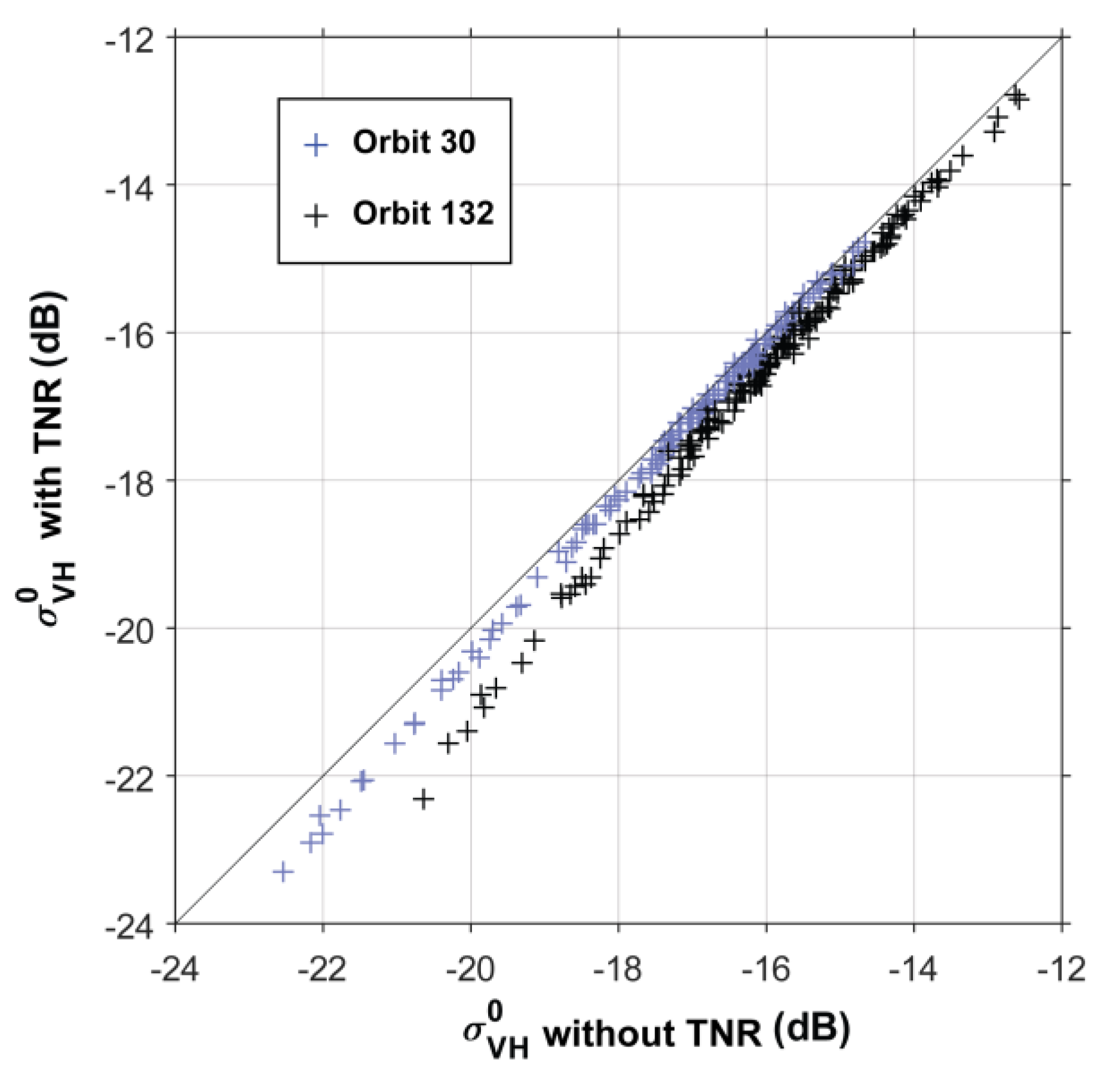
4.3.2. Impact of Thermal Noise Removal (TNR) on Backscattering Coefficients and on Mass Retrieval
4.4. What Is the Impact of an Intercrop?
5. Conclusions
Author Contributions
Funding
Acknowledgments
Conflicts of Interest
References
- Béziat, P.; Ceschia, E.; Dedieu, G. Carbon balance of a three crop succession over two cropland sites in South West France. Agric. For. Meteorol. 2009, 149, 1628–1645. [Google Scholar] [CrossRef]
- Ceschia, E.; Beziat, P.; Dejoux, J.; Aubinet, M.; Bernhofer, C.; Bodson, B.; Buchmann, N.; Carrara, A.; Cellier, P.; Di Tommasi, P.; et al. Management effects on net ecosystem carbon and GHG budgets at European crop sites. Agric. Ecosyst. Environ. 2010, 139, 363–383. [Google Scholar] [CrossRef]
- Hansen, E.; Djurhuus, J. Nitrate leaching as influenced by soil tillage and catch crop. Soil Tillage Res. 1997, 41, 203–219. [Google Scholar] [CrossRef]
- Ward, P.; Flower, K.; Cordingley, N.; Weeks, C.; Micin, S. Soil water balance with cover crops and conservation agriculture in a Mediterranean climate. Field Crop. Res. 2012, 132, 33–39. [Google Scholar] [CrossRef]
- Bastiaanssen, W.G.; Molden, D.J.; Makin, I.W. Remote sensing for irrigated agriculture: Examples from research and possible applications. Agric. Water Manag. 2000, 46, 137–155. [Google Scholar] [CrossRef]
- Kalluri, S.; Gilruth, P.; Bergman, R. The potential of remote sensing data for decision makers at the state, local and tribal level: Experiences from NASA’s Synergy program. Environ. Sci. Policy 2003, 6, 487–500. [Google Scholar] [CrossRef]
- Seelan, S.K.; Laguette, S.; Casady, G.M.; Seielstad, G.A. Remote sensing applications for precision agriculture: A learning community approach. Remote Sens. Environ. 2003, 88, 157–169. [Google Scholar] [CrossRef]
- Drusch, M.; Del Bello, U.; Carlier, S.; Colin, O.; Fernandez, V.; Gascon, F.; Hoersch, B.; Isola, C.; Laberinti, P.; Martimort, P.; et al. Sentinel-2: ESA’s Optical High-Resolution Mission for GMES Operational Services. Remote Sens. Environ. 2012, 120, 25–36. [Google Scholar] [CrossRef]
- Roy, D.P.; Wulder, M.A.; Loveland, T.R.; Woodcock, C.E.; Allen, R.G.; Anderson, M.C.; Helder, D.; Irons, J.R.; Johnson, D.M.; Kennedy, R.; et al. Landsat-8: Science and product vision for terrestrial global change research. Remote Sens. Environ. 2014, 145, 154–172. [Google Scholar] [CrossRef]
- Torres, R.; Snoeij, P.; Geudtner, D.; Bibby, D.; Davidson, M.; Attema, E.; Potin, P.; Rommen, B.; Floury, N.; Brown, M.; et al. GMES Sentinel-1 mission. Remote Sens. Environ. 2012, 120, 9–24. [Google Scholar] [CrossRef]
- Baghdadi, N.; Boyer, N.; Todoroff, P.; El Hajj, M.; Bégué, A. Potential of SAR sensors TerraSAR-X, ASAR/ENVISAT and PALSAR/ALOS for monitoring sugarcane crops on Reunion Island. Remote Sens. Environ. 2009, 113, 1724–1738. [Google Scholar] [CrossRef]
- Fieuzal, R.; Baup, F.; Marais-Sicre, C. Monitoring Wheat and Rapeseed by Using Synchronous Optical and Radar Satellite Data—From Temporal Signatures to Crop Parameters Estimation. Adv. Remote Sens. 2013, 2, 162–180. [Google Scholar] [CrossRef]
- Fieuzal, R.; Baup, F.; Marais-Sicre, C. Sensitivity of TERRASAR-X, RADARSAT-2 and ALOS Satellite Radar Data to Crop Variables. In Proceedings of the Geoscience and Remote Sensing Symposium (IGARSS), Munich, Germany, 22–27 July 2012; pp. 3740–3743. [Google Scholar]
- McNairn, H.; Champagne, C.; Shang, J.; Holmstrom, D.; Reichert, G. Integration of optical and Synthetic Aperture Radar (SAR) imagery for delivering operational annual crop inventories. ISPRS J. Photogramm. Remote Sens. 2009, 64, 434–449. [Google Scholar] [CrossRef]
- Betbeder, J.; Fieuzal, R.; Philippets, Y.; Ferro-Famil, L.; Baup, F. Contribution of multitemporal polarimetric synthetic aperture radar data for monitoring winter wheat and rapeseed crops. J. Appl. Remote Sens. 2016, 10, 026020. [Google Scholar] [CrossRef]
- Betbeder, J.; Fieuzal, R.; Baup, F. Assimilation of LAI and Dry Biomass Data from Optical and SAR Images into an Agro-Meteorological Model to Estimate Soybean Yield. IEEE J. Sel. Top. Appl. Earth Obs. Remote Sens. 2016, 9, 2540–2553. [Google Scholar] [CrossRef]
- Zribi, M.; Le Hégarat-Mascle, S.; Ottlé, C.; Kammoun, B.; Guerin, C. Surface soil moisture estimation from the synergistic use of the (multi-incidence and multi-resolution) active microwave ERS Wind Scatterometer and SAR data. Remote Sens. Environ. 2003, 86, 30–41. [Google Scholar] [CrossRef]
- Battude, M.; Al Bitar, A.; Brut, A.; Tallec, T.; Huc, M.; Cros, J.; Weber, J.-J.; Lhuissier, L.; Simonneaux, V.; Demarez, V. Modeling water needs and total irrigation depths of maize crop in the south west of France using high spatial and temporal resolution satellite imagery. Agric. Water Manag. 2017, 189, 123–136. [Google Scholar] [CrossRef]
- Fieuzal, R.; Duchemin, B.; Jarlan, L.; Zribi, M.; Baup, F.; Merlin, O.; Hagolle, O.; Garatuza-Payan, J. Combined use of optical and radar satellite data for the monitoring of irrigation and soil moisture of wheat crops. Hydrol. Earth Syst. Sci. 2011, 15, 1117–1129. [Google Scholar] [CrossRef]
- Sicre, C.M.; Baup, F.; Fieuzal, R. Determination of the crop row orientations from Formosat-2 multi-temporal and panchromatic images. ISPRS J. Photogramm. Remote Sens. 2014, 94, 127–142. [Google Scholar] [CrossRef]
- Yang, H.; Chen, E.; Li, Z.; Zhao, C.; Yang, G.; Pignatti, S.; Casa, R.; Zhao, L. Wheat lodging monitoring using polarimetric index from RADARSAT-2 data. Int. J. Appl. Earth Obs. Geoinf. 2015, 34, 157–166. [Google Scholar] [CrossRef]
- Haboudane, D. Hyperspectral vegetation indices and novel algorithms for predicting green LAI of crop canopies: Modeling and validation in the context of precision agriculture. Remote Sens. Environ. 2004, 90, 337–352. [Google Scholar] [CrossRef]
- Claverie, M.; Demarez, V.; Duchemin, B.; Hagolle, O.; Ducrot, D.; Marais-Sicre, C.; Dejoux, J.-F.; Huc, M.; Keravec, P.; Béziat, P.; et al. Maize and sunflower biomass estimation in southwest France using high spatial and temporal resolution remote sensing data. Remote Sens. Environ. 2012, 124, 844–857. [Google Scholar] [CrossRef]
- Fang, H.; Liang, S.; Hoogenboom, G.; Teasdale, J.; Cavigelli, M. Corn-yield estimation through assimilation of remotely sensed data into the CSM-CERES-Maize model. Int. J. Remote Sens. 2008, 29, 3011–3032. [Google Scholar] [CrossRef]
- Liu, J.; Pattey, E.; Miller, J.R.; McNairn, H.; Smith, A.; Hu, B. Estimating crop stresses, aboveground dry biomass and yield of corn using multi-temporal optical data combined with a radiation use efficiency model. Remote Sens. Environ. 2010, 114, 1167–1177. [Google Scholar] [CrossRef]
- Lobell, D.B.; Asner, G.P.; Ortiz-Monasterio, J.; Benning, T.L. Remote sensing of regional crop production in the Yaqui Valley, Mexico: Estimates and uncertainties. Agric. Ecosyst. Environ. 2003, 94, 205–220. [Google Scholar] [CrossRef]
- Moulin, S.; Bondeau, A.; Delécolle, R. Combining agricultural crop models and satellite observations: From field to regional scales. Int. J. Remote Sens. 1998, 19, 1021–1036. [Google Scholar] [CrossRef]
- Maas, S.J. GRAMI: A Crop Growth Model that Can Use Remotely Sensed Information; ARS—U.S. Department of Agriculture, Agricultural Research Service: Weslaco, TX, USA, 1992; Volume 91, 78p.
- Hsiao, T.C.; Heng, L.; Steduto, P.; Rojas-Lara, B.; Raes, D.; Fereres, E. AquaCrop—The FAO Crop Model to Simulate Yield Response to Water: III. Parameterization and Testing for Maize. Agron. J. 2009, 101, 448–459. [Google Scholar] [CrossRef]
- Duchemin, B.; Fieuzal, R.; Rivera, M.A.; Ezzahar, J.; Jarlan, L.; Rodriguez, J.C.; Hagolle, O.; Watts, C. Impact of Sowing Date on Yield and Water Use Efficiency of Wheat Analyzed through Spatial Modeling and FORMOSAT-2 Images. Remote Sens. 2015, 7, 5951–5979. [Google Scholar] [CrossRef]
- Duchemin, B.; Maisongrande, P.; Boulet, G.; Benhadj, I. A simple algorithm for yield estimates: Evaluation for semi-arid irrigated winter wheat monitored with green leaf area index. Environ. Model. Softw. 2008, 23, 876–892. [Google Scholar] [CrossRef]
- Dente, L.; Satalino, G.; Mattia, F.; Rinaldi, M. Assimilation of leaf area index derived from ASAR and MERIS data into CERES-Wheat model to map wheat yield. Remote Sens. Environ. 2008, 112, 1395–1407. [Google Scholar] [CrossRef]
- Fieuzal, R.; Baup, F.; Sicre, C.M. Estimation of corn yield using multi-temporal optical and radar satellite data and artificial neural networks. Int. J. Appl. Earth Obs. Geoinf. 2017, 57, 14–23. [Google Scholar] [CrossRef]
- Baup, F.; Villa, L.; Fieuzal, R.; Ameline, M. Sensitivity of X-Band (σ0, γ) and Optical (NDVI) Satellite Data to Corn Biophysical Parameters. Adv. Remote Sens. 2016, 5, 103–117. [Google Scholar] [CrossRef]
- Ameline, M.; Fieuzal, R.; Betbeder, J.; Berthoumieu, J.F.; Baup, F. Estimation of Corn Yield by Assimilating SAR and Optical Time Series into a Simplified Agro-Meteorological Model: From Diagnostic to Forecast. IEEE J. Sel. Top. Appl. Earth Obs. Remote Sens. 2018, 11, 4747–4760. [Google Scholar] [CrossRef]
- Rinaldi, M.; Satalino, G.; Mattia, F.; Balenzano, A.; Perego, A.; Acutis, M.; Ruggieri, S. Assimilation of COSMO-SkyMed-derived LAI maps into the AQUATER crop growth simulation model. Capitanata (Southern Italy) case study. Eur. J. Remote Sens. 2013, 46, 891–908. [Google Scholar] [CrossRef]
- Veloso, A.; Mermoz, S.; Bouvet, A.; Le Toan, T.; Planells, M.; Dejoux, J.-F.; Ceschia, E. Understanding the temporal behavior of crops using Sentinel-1 and Sentinel-2-like data for agricultural applications. Remote Sens. Environ. 2017, 199, 415–426. [Google Scholar] [CrossRef]
- Monteith, J.L.; Moss, C.J.; Cooke, G.W.; Pirie, N.W.; Bell, G.D.H. Climate and the efficiency of crop production in Britain. Philos. Trans. R. Soc. Lond. B Biol. Sci. 1977, 281, 277–294. [Google Scholar] [CrossRef]
- Maas, S.J. Parameterized Model of Gramineous Crop Growth: I. Leaf Area and Dry Mass Simulation. Agron. J. 1993, 85, 348–353. [Google Scholar] [CrossRef]
- Sánchez, B.; Rasmussen, A.; Porter, J.R. Temperatures and the growth and development of maize and rice: A review. Glob. Chang. Biol. 2014, 20, 408–417. [Google Scholar] [CrossRef] [PubMed]
- Battude, M.; Al Bitar, A.; Morin, D.; Cros, J.; Huc, M.; Sicre, C.M.; Le Dantec, V.; Demarez, V. Estimating maize biomass and yield over large areas using high spatial and temporal resolution Sentinel-2 like remote sensing data. Remote Sens. Environ. 2016, 184, 668–681. [Google Scholar] [CrossRef]
- Fieuzal, R.; Sicre, C.M.; Baup, F. Estimation of Sunflower Yield Using a Simplified Agrometeorological Model Controlled by Optical and SAR Satellite Data. IEEE J. Sel. Top. Appl. Earth Obs. Remote Sens. 2017, 10, 5412–5422. [Google Scholar] [CrossRef]
- Baret, F.; Hagolle, O.; Geiger, B.; Bicheron, P.; Miras, B.; Huc, M.; Berthelot, B.; Niño, F.; Weiss, M.; Samain, O.; et al. LAI, fAPAR and fCover CYCLOPES global products derived from VEGETATION. Remote Sens. Environ. 2007, 110, 275–286. [Google Scholar] [CrossRef]
- Oh, Y. Quantitative retrieval of soil moisture content and surface roughness from multipolarized radar observations of bare soil surfaces. IEEE Trans. Geosci. Remote Sens. 2004, 42, 596–601. [Google Scholar] [CrossRef]
- Gao, S.; Niu, Z.; Huang, N.; Hou, X. Estimating the Leaf Area Index, height and biomass of maize using HJ-1 and RADARSAT-2. Int. J. Appl. Earth Obs. Geoinf. 2013, 24, 1–8. [Google Scholar] [CrossRef]
- Macelloni, G.; Paloscia, S.; Pampaloni, P.; Marliani, F.; Gai, M. The relationship between the backscattering coefficient and the biomass of narrow and broad leaf crops. IEEE Trans. Geosci. Remote Sens. 2001, 39, 873–884. [Google Scholar] [CrossRef]
- Pinter, P.J., Jr.; Hatfield, J.L.; Schepers, J.S.; Barnes, E.M.; Moran, M.S.; Daughtry, C.S.T.; Upchurch, D.R. Remote Sensing for Crop Management. Photogramm. Eng. Remote Sens. 2003, 69, 647–664. [Google Scholar] [CrossRef]
- Ban, Y. Orbital effects on ERS-1 SAR temporal backscatter profiles of agricultural crops. Int. J. Remote Sens. 1998, 19, 3465–3470. [Google Scholar] [CrossRef]
- Joseph, A.T.; van der Velde, R.; O’Neill, P.E.; Lang, R.; Gish, T. Effects of corn on C- and L-band radar backscatter: A correction method for soil moisture retrieval. Remote Sens. Environ. 2010, 114, 2417–2430. [Google Scholar] [CrossRef]
- O’Keeffe, K. Maize Growth & Development; State of New South Wales through NSW Department of Primary Industries; NSW Department of Primary Industries: Orange, Australia, 2009; ISBN 978-0-7347-1955-3.
- Çakir, R. Effect of water stress at different development stages on vegetative and reproductive growth of corn. Field Crop. Res. 2004, 89, 1–16. [Google Scholar] [CrossRef]
- Denmead, O.T.; Shaw, R.H. The Effects of Soil Moisture Stress at Different Stages of Growth on the Development and Yield of Corn1. Agron. J. 1960, 52, 272–274. [Google Scholar] [CrossRef]
- Vollrath, A.; Lindquist, E.; Jonckheere, I.; Pekkarinen, A. Open Foris SAR Toolkit-Free and Open Source Command Line Utilities for Automatized SAR Data Pre-Processing. In Proceedings of the Living Planet Symposium 2016, Prague, Czech Republic, 9–13 May 2016; Volume 740, p. 31, ISBN 978-92-9221-305-3. [Google Scholar]
- Gorelick, N.; Hancher, M.; Dixon, M.; Ilyushchenko, S.; Thau, D.; Moore, R. Google Earth Engine: Planetary-scale geospatial analysis for everyone. Remote Sens. Environ. 2017, 202, 18–27. [Google Scholar] [CrossRef]
- Miranda, N.; Hajduch, G. Masking “No-Value” Pixels on GRD Products Generated by the Sentinel-1 ESA IPF. Issue 2.1, Reference MPC-0243. 2018, p. 14. Available online: https://sentinel.esa.int/documents/247904/2142675/Sentinel-1-masking-no-value-pixels-grd-products-note (accessed on 21 August 2019).
- Miranda, N.; Meadows, P.J. Radiometric Calibration of S-1 Level-1 Products Generated by the S-1 IPF. Technical Note; Reference ESA-EOPG-CSCOP-TN-0002, Issue 1. 2015. Available online: https://sentinel.esa.int/documents/247904/685163/S1-Radiometric-Calibration-V1.0.pdf (accessed on 21 August 2019).
- Lee, J.S. Refined filtering of image noise using local statistics. Comput. Graph. Image Process. 1981, 15, 380–389. [Google Scholar] [CrossRef]


| Field ID | Date of Sowing | Date of Harvest (doy/°C day) | Number of Samples | Date of Sampling (doy/°C day) |
|---|---|---|---|---|
| F1 | 102 | 278/2453 | 7 | (133/214, 148/352, 169/599, 195/985, 215/1299, 232/1574, 266/2095) |
| F2 | 104 | 281/2264 | 6 | (133/201, 169/586, 195/971, 215/1285, 232/1561, 266/2081) |
| F3 | 87 | 273/2261 | 6 | (133/292, 169/677, 195/1063, 215/1377, 232/1652, 266/2173) |
| F4 | 102 | 278/2453 | 7 | (133/214, 148/352, 169/599, 195/985, 215/1299, 232/1574, 266/2095) |
| Parameter | Definition | Domain of Variation | Unit |
|---|---|---|---|
| PlA | Partition-to-leaf function | 0.05–0.5 | - |
| PlB | Partition-to-leaf function | 10−5–10−2 | - |
| Stt | Temperature sum for senescence | 0–2000 | °C day |
| Rs | Rate of senescence | 0–105 | °C |
| D0 | Day0 | 90–250 | day |
| ELUE | Effective light-use efficiency | 0.5–6 | g.MJ−1 |
| Parameter | Value |
|---|---|
| PlA | 0.08 |
| PlB | 3.0 × 10⁻³ |
| Stt | 1361 |
| Rs | 3569 |
| D0 | 142 |
| ELUE | 3.98 |
| Target Output | n | R² | a | b | RMSE | rRMSE (%) |
|---|---|---|---|---|---|---|
| GAI | 9 | 0.99 | 0.97 | −0.08 | 0.08 | 10.58 |
| EDM | 7 | 0.96 | 0.99 | −0.05 | 0.82 | 27.65 |
| PDM | 7 | 0.97 | 0.95 | 0.10 | 0.45 | 14.48 |
| TDM | 7 | 0.96 | 0.96 | 0.12 | 1.17 | 19.35 |
| Parameter | F1 | F2 | F3 | F4 | F5 | F6 | F7 | F8 |
|---|---|---|---|---|---|---|---|---|
| D0 (DoY) | 150 | 157 | 137 | 143 | 104 | 133 | 132 | 144 |
| ELUE (g.MJ−1) | 4.32 | 4.40 | 3.93 | 3.79 | 3.14 | 3.67 | 3.73 | 4.12 |
| n | R² | a | b | RMSE | rRMSE | ||
|---|---|---|---|---|---|---|---|
| with TNR and without speckle filter | EDM | 19 | 0.93 | 0.87 | 0.11 | 1.07 | 28.70 |
| PDM | 19 | 0.90 | 0.65 | 0.16 | 0.59 | 15.67 | |
| TDM | 19 | 0.92 | 0.85 | 0.14 | 1.77 | 23.56 | |
| with TNR and with speckle filter | EDM | 19 | 0.95 | 0.96 | 0.08 | 0.94 | 25.32 |
| PDM | 19 | 0.68 | 0.65 | 0.92 | 1.23 | 32.74 | |
| TDM | 19 | 0.95 | 0.92 | 1.09 | 1.46 | 19.44 | |
| without TNR | EDM | 19 | 0.94 | 1.81 | 0.57 | 2.19 | 58.57 |
| PDM | 19 | 0.36 | 0.99 | 3.34 | 3.72 | 98.77 | |
| TDM | 19 | 0.87 | 1.65 | 4.02 | 4.46 | 59.40 |
© 2019 by the authors. Licensee MDPI, Basel, Switzerland. This article is an open access article distributed under the terms and conditions of the Creative Commons Attribution (CC BY) license (http://creativecommons.org/licenses/by/4.0/).
Share and Cite
Baup, F.; Ameline, M.; Fieuzal, R.; Frappart, F.; Corgne, S.; Berthoumieu, J.-F. Temporal Evolution of Corn Mass Production Based on Agro-Meteorological Modelling Controlled by Satellite Optical and SAR Images. Remote Sens. 2019, 11, 1978. https://doi.org/10.3390/rs11171978
Baup F, Ameline M, Fieuzal R, Frappart F, Corgne S, Berthoumieu J-F. Temporal Evolution of Corn Mass Production Based on Agro-Meteorological Modelling Controlled by Satellite Optical and SAR Images. Remote Sensing. 2019; 11(17):1978. https://doi.org/10.3390/rs11171978
Chicago/Turabian StyleBaup, Frédéric, Maël Ameline, Rémy Fieuzal, Frédéric Frappart, Samuel Corgne, and Jean-François Berthoumieu. 2019. "Temporal Evolution of Corn Mass Production Based on Agro-Meteorological Modelling Controlled by Satellite Optical and SAR Images" Remote Sensing 11, no. 17: 1978. https://doi.org/10.3390/rs11171978
APA StyleBaup, F., Ameline, M., Fieuzal, R., Frappart, F., Corgne, S., & Berthoumieu, J.-F. (2019). Temporal Evolution of Corn Mass Production Based on Agro-Meteorological Modelling Controlled by Satellite Optical and SAR Images. Remote Sensing, 11(17), 1978. https://doi.org/10.3390/rs11171978