Article

Fast and Effective Techniques for LWIR Radiative Transfer Modeling: A Dimension-Reduction Approach

1
Department of Electrical and Computer Engineering, Air Force Institute of Technology, Wright-Patterson AFB, OH 45433, USA
2
Department of Engineering Physics, Air Force Institute of Technology, Wright-Patterson AFB, OH 45433, USA
*
Author to whom correspondence should be addressed.
Current address: Air Force Institute of Technology, Wright-Patterson AFB, OH 45433, USA.
These authors contributed equally to this work.
Remote Sens. 2019, 11(16), 1866; https://doi.org/10.3390/rs11161866
Submission received: 3 June 2019 / Revised: 31 July 2019 / Accepted: 2 August 2019 / Published: 9 August 2019
(This article belongs to the Special Issue Robust Multispectral/Hyperspectral Image Analysis and Classification)

Abstract

:
The increasing spatial and spectral resolution of hyperspectral imagers yields detailed spectroscopy measurements from both space-based and airborne platforms. These detailed measurements allow for material classification, with many recent advancements from the fields of machine learning and deep learning. In many scenarios, the hyperspectral image must first be corrected or compensated for atmospheric effects. Radiative Transfer (RT) computations can provide look up tables (LUTs) to support these corrections. This research investigates a dimension-reduction approach using machine learning methods to create an effective sensor-specific long-wave infrared (LWIR) RT model. The utility of this approach is investigated emulating the Mako LWIR hyperspectral sensor ( Δ λ 0.044   μ m , Δ ν ˜ 3.9 cm 1 ). This study employs physics-based metrics and loss functions to identify promising dimension-reduction techniques and reduce at-sensor radiance reconstruction error. The derived RT model shows an overall root mean square error (RMSE) of less than 1 K across reflective to emissive grey-body emissivity profiles.

Graphical Abstract

1. Introduction

Next-generation hyperspectral imagers continue to improve in both spatial and spectral resolution with increasingly lower noise-equivalent spectral radiance (NESR) values, presenting unique opportunities in efficiently characterizing pixel materials [1]. A pixel in a hyperspectral image can be represented as a vector across all spectral channels, producing a three-dimensional data cube for an entire image, width by height by spectral channel [2]. Hyperspectral imagers have been deployed in both airborne and space-based platforms with uses ranging from precision agriculture to search and rescue operations [3]. The spectral bands making up a hyperspectral cube can span from the visible to the LWIR, sampled across hundreds of narrow spectral channels [4]. The visible to short-wave infrared (SWIR) (0.4– 3.0 μ m ) is dominated by scattering while the LWIR (5.0– 14.0 μ m ) is dominated by material emission [5]. The atmospheric state—which includes the altitude-dependent temperature and pressure; how column water vapor content, carbon dioxide, ozone, and other trace gases are distributed vertically; the kind and size distributions of various aerosols—has a significant impact on the at-sensor radiance. Understanding and accounting for these atmospheric effects is critical for quantitative exploitation of hyperspectral imagery, especially in the domain of material identification.
RT calculations convert the atmospheric state parameters—temperature, water, and ozone values as functions of altitude or pressure—into spectral radiances observed at the sensor by discretizing the atmosphere into thin, homogeneous layers. At each layer, high spectral resolution RT calculations (e.g., LBLRTM) are performed, or approximations thereof (e.g., MODTRAN). Due to the large number of discrete absorption lines of the many trace gases in the atmosphere, millions of calculations are required to model a sensor’s entire spectral range with high fidelity [6]. This computational complexity is the primary bottleneck in remote sensing retrieval problems, often limiting the use of RT models in real-time data analysis.
To avoid the high computational cost of line-by-line RT calculations, approximate RT models are used to increase computational speed while trading off accuracy [7]. One of the most widely used approaches to improve RT computation time is the correlated-k method, which divides opaque spectrum into a subset of b bands and then applies a weighting k to these bands, dependent on the opacity distribution of the b bands [8].
Similar to the weighting scheme employed in the correlated-k method, principal component analysis (PCA) has also been implemented to reduce RT computation time [6]. PCA can be applied on the input space (atmospheric state parameters) and/or on the output space (spectral radiances) to reduce RT computational time. In [9], PCA was applied to atmospheric state parameters for quickly estimating spectra in the O 2 A-band with an accuracy of 0.3% compared to multi-stream methods with a 10-fold reduction in computation time. In [6], PCA was applied to database spectral radiances identifying a lower-dimensional space of only a few hundred components compared to the thousands of dimensions in the original data space. Implementations such as principal component radiative transfer model (PCRTM) [6] or principal component radiative transfer for TOVs (PCRTTOV) [10] perform RT computations for a subset of bands and map these to the low-dimensional space to create the highly efficient RT model. In [11], PCA was considered on both the input atmospheric parameter space and the output spectral radiance space to further reduce computational time with an overall error of 0.05%.
This study focuses on efficient conversion of atmospheric state parameters into spectral radiances for the LWIR domain using neural network approaches. This is achieved by performing dimension reduction on the output spectral radiance space (transmittance, upwelling radiance, and downwelling radiance (TUD) vectors) and then fitting a neural network to sample the low-dimensional space. Our approach is similar to PCRTM [6]; however, we use autoencoder networks for the dimension-reduction step instead of PCA.
The most salient contributions and findings of this research include:
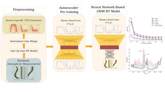
  • Employing machine learning techniques which: (1) are computationally faster than correlated-k calculation methods; (2) reduce the dimension of both the TUD and atmospheric state vectors; (3) produce the desirable latent-space-similarity property such that small deviations in the low-dimension latent space result in small deviations in the high-dimension TUD
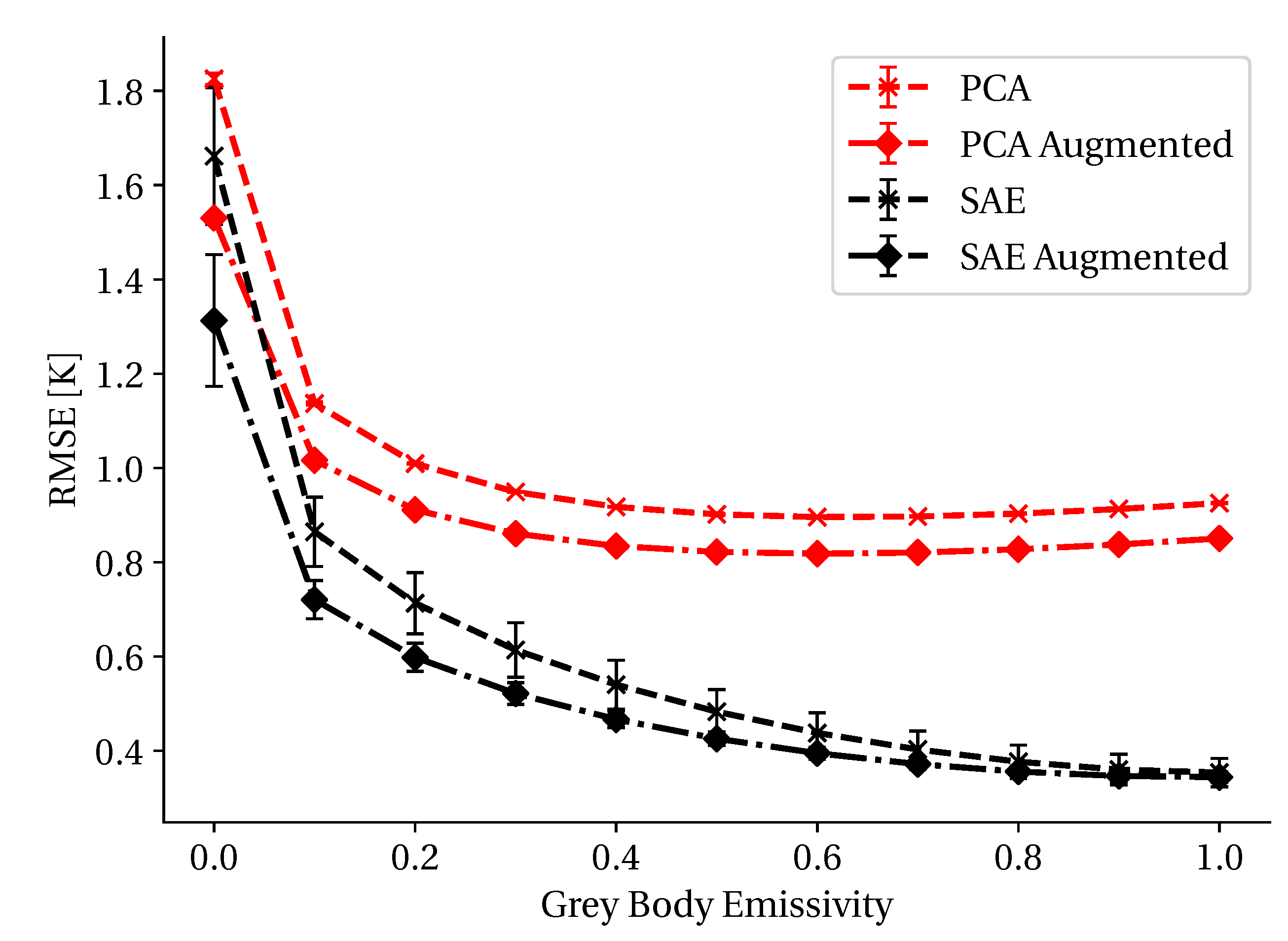
  • Developing a data augmentation method using PCA and Gaussian mixture models (GMMs) on real atmospheric measurements that lead to improved model training and generalizability
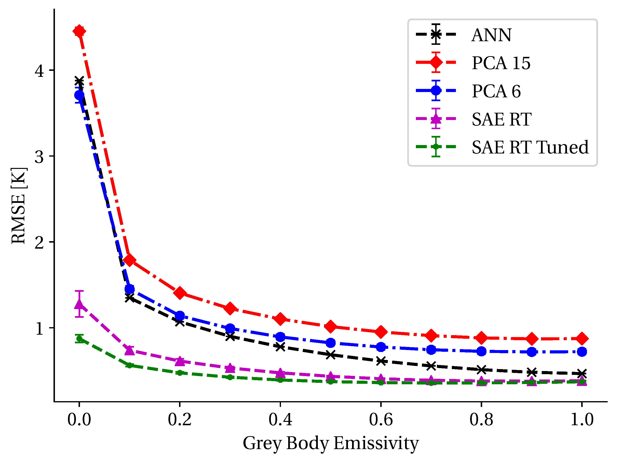
  • Improving machine learning model training by introducing a physics-based loss function which encourages better fit models than traditional loss functions based on mean squared error
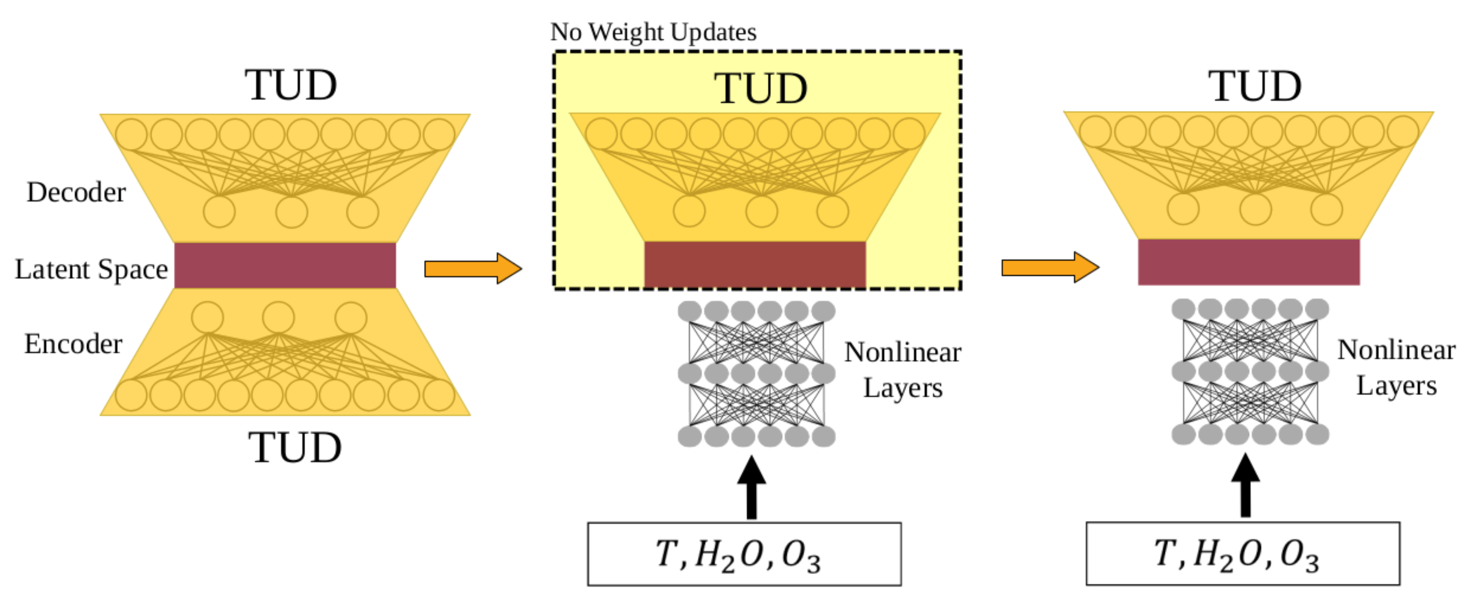
  • Demonstrating an effective autoencoder (AE) pre-training strategy that leverages the local-similarity properties of the latent space to reproduce TUDs from atmospheric state vectors
Together, these contributions form the basis of a novel method for efficient and effective RT modeling, using a small number of parameters.

Background

Atmospheric compensation techniques estimate the atmospheric effects imposed on the at-sensor signal, leading to atmospherically corrected data for material classification and identification. In the LWIR, the simplest RT model for describing the at-sensor radiance, L ( λ ) , from a diffuse (lambertian) thermal emitter and scatterer, can be expressed as [3]:
L ( λ ) = τ ( λ ) ϵ ( λ ) B ( λ , T ) + 1 ϵ ( λ ) L d ( λ ) + L a ( λ )
λ : wavelength T : material temperature τ ( λ ) : atmospheric transmission ϵ ( λ ) : material emissivity B ( λ , T ) : Planckian distribution L d ( λ ) : downwelling atmospheric radiance L a ( λ ) : atmospheric path ( upwelling ) radiance
Both τ and L a are specific to the line of sight between the sensor and the surface, whereas L d represents a cosine-weighted average of the downwelling radiance for the hemisphere above the surface. Planck’s blackbody distribution function, B ( λ , T ) , is given by
B ( λ , T ) = 2 h c 2 λ 5 1 e h c / λ k T 1
where k is Boltzmann’s constant, c is the speed of light and h is Planck’s constant. Atmospheric compensation recovers the surface leaving radiance L s ( λ ) by estimating τ ( λ ) and L a ( λ ) in Equation (1) as shown in Equation (3).
L s ( λ ) = ϵ ( λ ) B ( λ , T ) + 1 ϵ ( λ ) L d ( λ )
One of the most popular LWIR atmospheric compensation techniques is the In-Scene Atmospheric Compensation (ISAC) method which first identifies blackbody pixels within the scene to estimate τ ( λ ) and L a ( λ ) [12]. By using only pixel spectra from blackbodies, the surface leaving radiance is equivalent to Planck’s blackbody distribution and the simplified LWIR at-sensor radiance can be expressed as
L ( λ ) ϵ ( λ ) 1 = τ ( λ ) B ( λ , T ) + L a ( λ ) .
Under the assumption that distinct blackbody pixels can be identified, and their temperatures known, a linear fit can be performed across all spectral channels to identify τ ( λ ) and L a ( λ ) . In practice, temperatures estimates are made in the most transmissive part of the at-sensor spectral radiance but they are often systematically biased since τ ( λ ) and L a ( λ ) are unknown and assumed to be 1 and 0, respectively, in that particular spectral channel λ . A common method to remove the biases introduced into τ and L a by inaccurate surface temperatures relies on spectral analysis near the isolated water absorption feature near 11.73 μ m . This method is very similar to the Autonomous Atmospheric Compensation (AAC) method, which estimates a transmittance ratio and an upwelling radiance parameter derived from the off- and on-resonance spectral values at the same isolated water band [13]. By assessing this water feature, both transmittance and path radiance contributions can be independently estimated, allowing the biased ISAC estimates of τ and L a to be fixed, or under further assumptions about the atmosphere, allowing full estimates of τ and L a to be made. To ensure algorithmic efficiency for both ISAC and AAC, precomputed look-up tables of τ ( λ ) and L a ( λ ) are forward-modeled with a RT model over a wide range of possible atmospheric water and temperature profiles. In the LWIR portion of the spectrum, Temperature-Emissivity Separation (TES) follows atmospheric compensation to estimate material emissivity and surface temperature from L s ( λ ) [14].
In this study, we conduct dimension reduction on the TUD vectors ( τ ( λ ) , L a ( λ ) , L d ( λ ) ) in Equation (1) which span a wide range of global atmospheric variability. Specifically, this research uses the Thermodynamic Initial Guess Retrieval (TIGR) database comprising myriad atmospheric conditions in the form of temperature, water vapor, and ozone profiles on a fixed pressure grid. The 2311 atmospheric profiles provided in the TIGR database are based on 80,000 radiosonde measurements collected worldwide [15,16]. The TIGR atmospheric profiles are first filtered for cloud-free conditions and then forward-modeled using the Line-by-Line Radiative Transfer Model (LBLRTM) (version 12.8) to create realistic TUD vectors which also span a broad range of atmospheric conditions.
Conducting dimension reduction on the TIGR-derived TUD vectors creates a low-dimensional representation that can be sampled to create new TUD vectors without the need for costly RT calculations. Research performed in [17] specifically considered a low-rank subspace of τ ( λ ) and L a ( λ ) for atmospheric compensation in the LWIR spectrum. They performed a singular value decomposition on representative τ ( λ ) and L a ( λ ) vectors generated by MODTRAN for a given seasonal model and flight altitude. Blackbody pixels were identified within a scene based on their projection onto these subspaces, thus providing a way to directly estimate transmittance and upwelling radiance for a scene. The neural network approach we take for TUD vector compression is not invertible; therefore, we cannot directly apply the approach outlined in [17] for atmospheric compensation. The RT model can assist the atmospheric compensation in [17], by quickly providing a wide range of transmittance and upwelling vectors to construct the low-rank subspaces.
Creating a low-dimensional TUD representation is also important for data augmentation applications, distinctly different from atmospheric compensation. To identify a material of interest, many augmented representations of that material through diverse atmospheric conditions can be created using a low-dimensional TUD representation. By providing many of the commonly investigated classification techniques augmented at-sensor data representative of diverse and realistic TUD vectors, atmospherically robust classification can be improved. This was the approach employed in [18], where a small neural network was trained to detect specific materials in the LWIR across varying atmospheric conditions. The neural network-based approaches investigated here offer a highly efficient method to generate realistic TUD vectors to support data augmentation.
Additionally, the utility of the low-dimensional representation is explored by mapping the atmospheric state (temperature, water vapor and ozone profiles) to the low-dimensional space, thus creating a highly efficient RT model. This RT model can be used for data augmentation as discussed above or to support model-based compensation techniques where hundreds of possible transmittance and upwelling vectors can be computed in real time, avoiding the use of precomputed look-up tables. By performing dimension reduction prior to fitting this mapping, similar atmospheric conditions cluster together in the low-dimensional space. Additionally, based on this clustering, small deviations in the low-dimensional space correspond to small changes in generated TUD vectors, further improving the mapping from atmospheric measurements to the low-dimensional space.
In the next section dimension-reduction techniques are reviewed and the TIGR dataset is explained in further detail. Metrics based on Equation (1) are also derived to ensure dimension-reduction techniques are correctly evaluated. Sampling of the low-dimensional TUD representation is also outlined to demonstrate the utility of these techniques and highlight the importance of latent-space-similarity where deviations in the latent space correspond to similar deviations in high-dimension TUD space.
Following the methodology section, results are presented comparing dimension-reduction performance derived from the TIGR data and an augmented version of the TIGR data. After confirming improved performance with the augmented data, a novel physics-based loss function is compared to mean squared error (MSE) to further improve dimension-reduction reconstruction error. Finally, a RT model is formulated from the dimension-reduction algorithms, showing the importance of the dimension-reduction pre-training step toward reduced TUD prediction error.

2. Methodology

This section first reviews the atmospheric measurement data and corresponding forward-modeled TUD vectors used for dimension reduction. Metrics for comparing the performance of each technique are also reviewed, with a focus on incorporating properties from the simplified RT model in Equation (1). A unique data augmentation scheme is also discussed to increase the number of TUD samples for model fitting.

2.1. Data

The TIGR database consists of 2311 atmospheres selected from over 80,000 worldwide radiosonde reports. These atmospheric conditions represent a broad range of conditions favorable for capturing atmospheric variations in remotely sensed data. Each sample contains temperature, water content and ozone at 43 discrete pressure levels ranging from the earth’s surface (1013 hPa) to > 30 km (<1 hPa) [15,16]. Cubic interpolation was used to upsample these profiles to 66 pressure levels, with finer sampling in the lower, most dense part of the atmosphere. Additionally, the profiles are grouped by air mass category such as polar, tropical, and mid-latitude. The entire TIGR data matrix shape is 2311 atmospheric profiles by 198 measurements, where the 66 pressure level measurements for temperature, water content, and ozone are concatenated.
By using atmospheric profiles that span nearly all expected atmospheric variability, RT can be conducted to generate TUD vectors encapsulating nearly every possible atmospheric scenario. The LBLRTM was used to create high-resolution TUD vectors; however, the spectral resolution must be downsampled for a particular sensor to ensure the dimension-reduction techniques are applicable to real-world sensor resolutions.
The LWIR Mako hyperspectral sensor is a high-performance, airborne sensor imaging across 7.8–13.4 μ m into 128 spectral channels with a noise-equivalent temperature difference of 0.02 K at 10 μ m and 300 K [1,19]. The high-resolution LBLRTM generated TUD vectors (11,513 spectral channels) are downsampled according to the Mako instrument line shape creating representative TUD vectors for this sensor. Additionally, the TUD vectors are generated to represent a sensor altitude of 3.3 k m . The result of this process is shown in Figure 1, where after downsampling, the TUD data matrix shape is 2311 samples by 384 spectral measurements ( τ ( λ ) , L a ( λ ) , L d ( λ ) concatenated). The goal of the dimension-reduction algorithms discussed next is to project the length 384 TUD vectors to a lower-dimensional space such that reconstruction error is minimized.

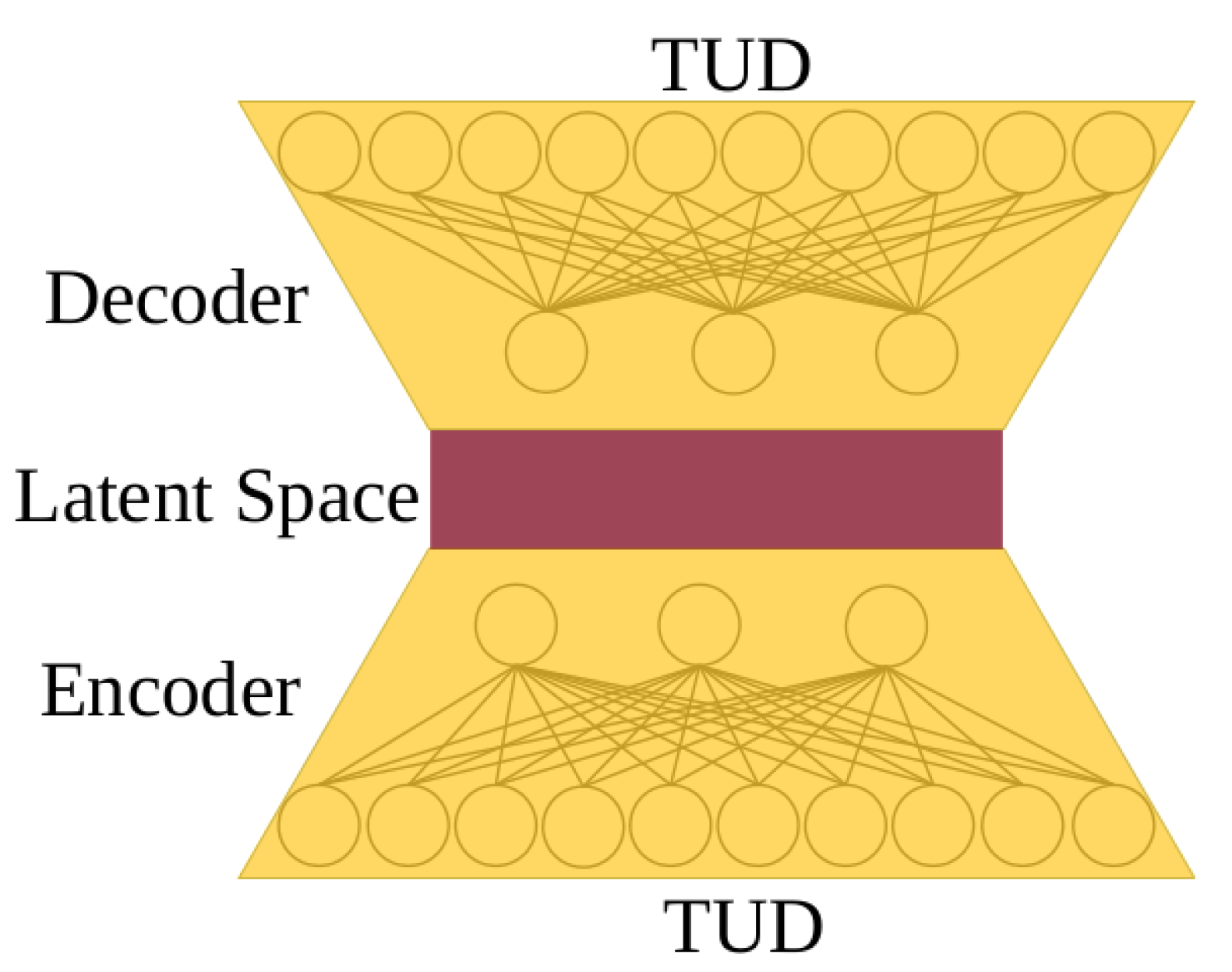
2.2. TUD Dimension-Reduction Techniques

PCA removes correlation from data by projecting it onto a new coordinate system which maximizes data variance. Let x i be a single measurement with P features and X be the data matrix containing N measurements such that X R N × P . To apply PCA to data matrix X , first an eigendecomposition is performed on the data covariance matrix C x such that
C x = A D A T
where the matrix A is an orthonormal square matrix consisting of P eigenvectors and D is a diagonal matrix consisting of the corresponding eigenvalues [20]. The eigenvalues are sorted in descending order and the L eigenvectors corresponding to the largest eigenvalues are kept, where L < < P . This selection is based on the cumulative sum of data variance explained with the eigenvectors. The smallest eigenvalue components are considered noise and have little impact on reconstructing the original signal. In this study, we will vary the number of L components to minimize reconstruction error. The subset of selected eigenvectors are used to linearly transform the data to the low-dimensional representation y R L by:
y i = A T x i .
An AE is a neural network designed for performing nonlinear compression by projecting data to a low-dimensional latent space, followed by nonlinear reconstruction from the latent space. An AE is composed of two networks to perform this operation: an encoder network and a decoder network. The encoder compresses the input data, x , into a lower-dimensional latent space, z , and the decoder reconstructs the data based on the latent space mapping into y [21]. Equations for these two transformations are
z = f ( W z x + b z ) y = f ( W y z + b y )
where x R d is the input data, z R l is the latent space representation with l d . The reconstructed data is y R d and b y and b z are the biases of the hidden and output layer layers, respectively. W z and W y are the weight matrices from the input to hidden layer and hidden layer to output layer, respectively. An AE diagram is shown in Figure 2 specifically for TUD compression and decompression using the encoder, decoder, and latent space nomenclature. This figure is only notional, and does not represent the number of nodes actually used in this study.
The AE predicted TUD vectors are compared to the LBLRTM generated TUD vectors through a loss function to determine model performance and update the weight matrices. The loss function used for measuring reconstruction error between TUD vectors is an important design variable influencing how the AE structures the latent space and ultimately what the network understands about TUD reconstruction. A commonly used loss function is MSE, calculated according to:
MSE = 1 K i = 1 K x i y i 2
where K equals the number of dimensions in the TUD vector, and x i and y i are the predicted and truth TUD vectors, respectively. MSE will be used in this study, but an additional loss function will be derived later based on the underlying LWIR RT model. In many applications, a series of hidden layers are used to create a latent space representation of the data. This architecture is commonly referred to as a stacked autoencoder (SAE), where the functions shown in Equation (6) are nested to include additional layers. The activation function, f, can be linear or nonlinear. A comprehensive search of activation functions found the Rectified Linear Unit (ReLU) [22] yielded the best results over functions such as hyperbolic tangent, sigmoid, exponential linear units, and scaled exponential linear units. The ReLU function used in this study is
RELU ( x ) = x , if x > 0 α x , if x < 0
where α controls how much information is passed through the network for negative inputs. This small slope increases information flow during backpropagation allowing more weights to be influenced by training samples [23].
The number of latent components is an important design parameter controlling model complexity and reconstruction performance. Using two latent components allows for visualizations of the latent space by overlaying measurement parameters such as surface temperature and total atmospheric water vapor content. For the PCA model, the first two components capture 99.50% of the data variance. Plotting just these two components shows a smoothly varying relationship between the components and these physical parameters as shown in Figure 3. Both the validation set (158 samples) and test set (176 samples) are plotted to highlight this underlying dependence on atmospheric conditions.
Similar plots are shown in Figure 4 when considering a 2 component SAE model. Interestingly, the SAE disperses the validation and test set points throughout the latent space which is beneficial for sampling the low-dimensional representation. Small changes in latent space components should result in small changes in the generated TUD vectors. This latent-space-similarity is an important property when fitting a sampling method to correctly identify a small number of components to generate a TUD vector. Small sampling errors should not result in large TUD deviations. Since it is difficult to visualize higher-dimension latent spaces, this property can be observed by fitting a small neural network to correctly predict the latent components for a known TUD.
The PCA model has little change in components 1 and 2 for cold, dry atmospheric conditions as shown by the tight clustering of these points. There appears to be a stronger dependence on component 2 for cold, dry atmospheres, while hot, humid conditions are dependent on both components. The SAE components are both influenced by surface temperature, while component 2 appears more dependent total water vapor content. Based on the preliminary results shown in Figure 3 and Figure 4, sampling the two-dimensional AE latent space will result in lower reconstruction error because of the tight clustering of cold dry atmospheric conditions shown in the PCA latent space. Using only two components results in large reconstruction error, therefore, we will consider additional latent components to cluster similar atmospheric conditions together in a low-dimensional space while minimizing reconstruction error.

2.3. Metrics

For all methods considered, the reconstruction error must be placed in context of the at-sensor radiance to provide meaningful reconstruction performance. At-sensor radiance errors are dependent on the material emissivity as shown in Equation (4) where downwelling radiance does not play a role in the total error. However, if the surface material is reflective ( ϵ ( λ ) = 0 ), the simplified LWIR RT equation becomes
L ( λ ) ϵ ( λ ) 0 = τ ( λ ) L d ( λ ) + L a ( λ )
where errors in τ ( λ ) and L d ( λ ) are now exaggerated. Using a standard metric, such as MSE, does not capture this dependence on material emissivity and provides misleading model performance for reflective versus emissive materials. A more appropriate metric for this domain considers the material emissivity in the at-sensor radiance error calculation.
For a test emissivity, ϵ t ( λ ) , the estimated at-sensor radiance, L ^ ( λ ) is calculated based on the reconstructed TUD vector. Additionally, the original TUD vector is used in conjunction with ϵ t ( λ ) to calculate the true at-sensor radiance L ( λ ) . The RMSE, E t , is calculated across all spectral channels such that
E t = 1 K i = 1 K L ( λ i ) L ^ ( λ i ) 2
where K represents the number of spectral channels and E t is now in radiance units representing the emissivity dependent RMSE. For the LWIR domain, errors are typically expressed in terms of temperature where conversion of radiance to brightness temperature is defined as [3]:
T B B ( λ ) = h c λ k ln 2 h c 2 λ 5 L ( λ ) + 1
By transforming at-sensor radiance to brightness temperature, the at-sensor error between L ^ ( λ ) and L ( λ ) can now be expressed in Kelvin. In general, reconstruction performance improves as ϵ t ( λ ) approaches 1.0 based on Equation (4). The actual emissivity values used are assumed grey bodies (spectrally flat) and linearly sampled between 0 and 1. Calculating the emissivity dependent RMSE provides additional information over standard MSE between predicted and truth TUD values. Model selection is performed based on performance across the entire emissivity domain resulting in lower error for reflective materials.
Constructing a model with low error across a range of emissivity values requires modifications to model training. As shown by the emissivity dependent RMSE metric, standard MSE will not provide sufficient information to properly update model weights. Instead, the loss function for training the SAE must include emissivity dependent information. The loss function must still be differentiable and result in stable training performance. To achieve this, we use the TUD MSE calculation for stabilized training, but also include an at-sensor radiance MSE dependent on material emissivity:
L ( x , y ) = 1 3 K i = 1 3 K x i y i 2 + γ M N j = 1 M i = 1 K L x ( λ i , ϵ j ) L ^ y ( λ i , ϵ j ) 2
where x is the truth TUD vector, y is the reconstructed TUD vector and K is the number of spectral bands. The terms L x ( λ i , ϵ j ) and L ^ y ( λ i , ϵ j ) represent the at-sensor radiance using the truth and predicted TUD vectors respectively. The at-sensor radiance loss is calculated using a linear sampling of M emissivity values between 0 and 1, noted by ϵ j in the loss calculation. A regularization term, γ , is included in Equation (11) to trade-off at-sensor radiance error and the TUD reconstruction error. In this study, we only consider γ = 1 ; however, future work will consider this additional hyperparameter in the network optimization.
By including a loss component for the at-sensor radiance, network weights are updated to minimize at-sensor radiance error rather than strictly TUD reconstruction error. This is an important additional constraint since material emissivity impacts the difficulty of the reconstruction problem as shown by Equation (8). The MSE component in Equation (11) is necessary to stabilize training since errors in one component of the TUD vector can cause a reduction in overall loss depending on material emissivity. In practice, training networks without the MSE component caused large deviations in loss values as the network weights tried to simultaneously optimize for a range of emissivity values.

2.4. Radiative Transfer Modeling

We consider the utility of the low-dimension TUD representation by applying it to the problem of RT modeling. Specifically, this section considers how to map atmospheric state vectors to the previously fit AE latent space. Our approach for creating the RT model is similar to pre-training performed in other domains such as AEs to create useful feature maps for classification [24]. Figure 5 displays an overview of the entire RT model training process. The first step in Figure 5 is the fitting of the TUD dimension-reduction technique already discussed.
Next, a sampling network is trained to correctly predict the latent space components using atmospheric state vectors as shown by the second step in Figure 5. During this step of the training process, no updates are made to the previously trained decoder network. Once the sampling network weights have converged, the entire RT model is trained end-to-end (third step in Figure 5), allowing small weight updates in both the sampling network and the decoder. We observed less than 200 iterations are needed for the final training step as network weights are nearly optimized for the TUD regression task. As shown later, we compare the results of this process to a fully connected neural network without the two pre-training steps shown in Figure 5.
Creating a RT model also highlights differences in the latent space construction among differing dimension-reduction techniques. Ideally, similar atmospheric conditions will form clusters in the low-dimensional space. Sampling anywhere within these clusters should result in similar TUD vectors reducing the impact of sampling errors. Additionally, small changes in generative model components should lead to small deviations in the generated TUD vectors. We found that pre-training an AE to reconstruct TUD vectors was useful for enforcing a similarity between generative model components and their corresponding TUD vectors. Both properties allow a sampling method to quickly learn a relationship between atmospheric measurements and the corresponding generative model components. Difficulties in sampling the latent space to generate TUD vectors may be the result of one or both properties not being satisfied.
The loss function for updating the nonlinear sampling layers is dependent on the dimension-reduction method used to form the latent space. For SAE dimension reduction, the loss function is simply the MSE calculated between predicted components and truth components. In this case, truth components are derived from the encoder model. For PCA, components are ordered according to the variance they capture, therefore, it is important for the sampling method to correctly predict components capturing higher variance. The loss function used in this case is a weighted MSE described as:
MSE PCA = 1 K i = 1 K w i ( x i y i ) 2
where w i corresponds to the percentage of variance (expressed as a fraction) captured by component i during the PCA fitting process. This scaling ensures a weighted reconstruction reflecting component importance. Next, TIGR data augmentation is discussed as more atmospheric measurement samples are needed to fit the large number of dimension-reduction model parameters.

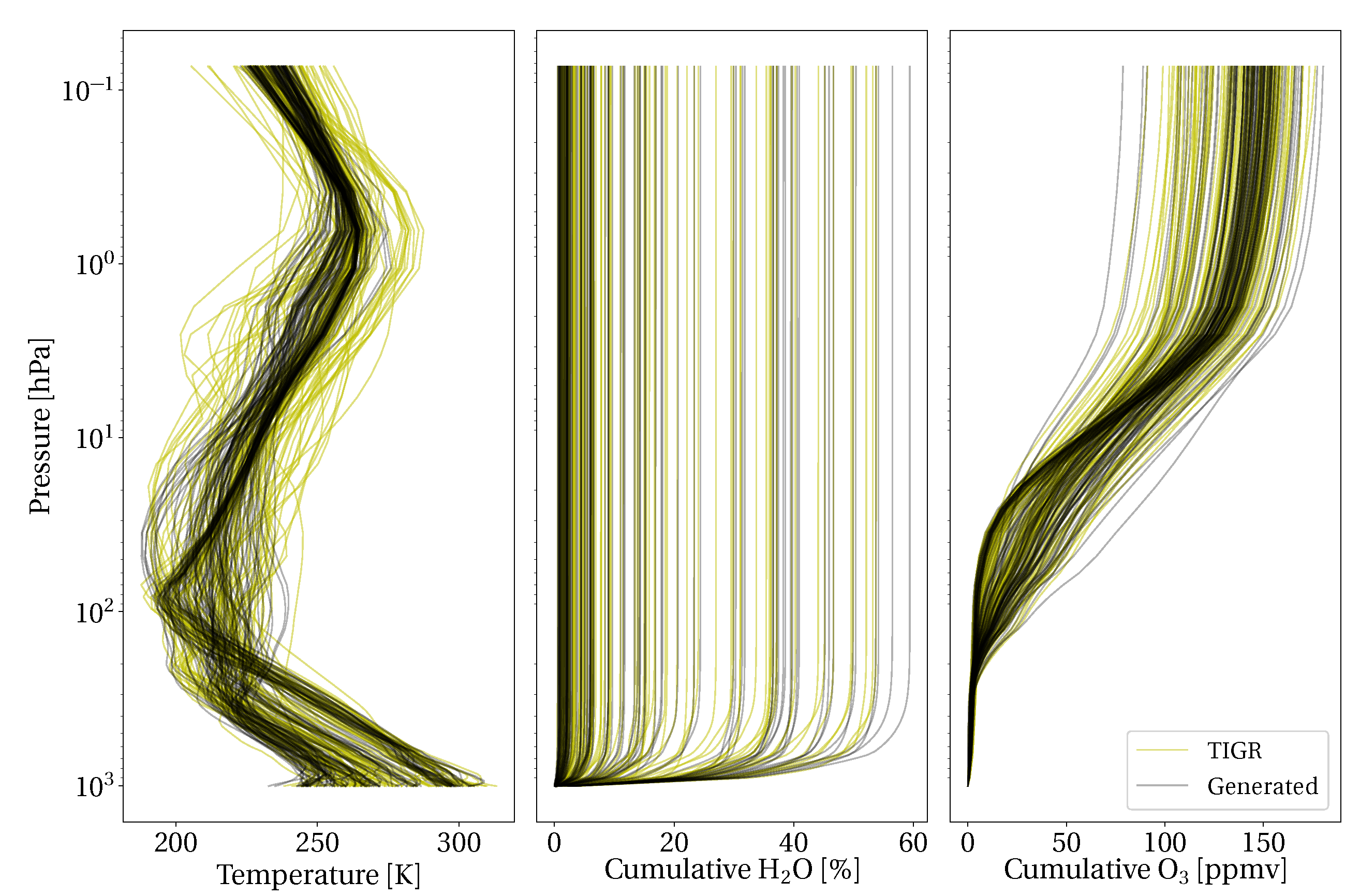
2.5. Atmospheric Measurement Augmentation

The 2311 TIGR atmospheric measurements span expected atmospheric variability, providing a set of basis measurements to fit dimension-reduction models. To accurately fit the thousands of weights within a neural network, additional TUD vectors are needed to interpolate between the TIGR samples. In this section, a data augmentation approach is introduced, resulting in over 11,000 new TUD vectors derived from the TIGR database.
This study will only consider cloud-free conditions requiring a relative humidity calculation to be performed on each TIGR measurement. Using a threshold of 96% relative humidity, we downselect the TIGR data to 1755 samples. Each remaining temperature, water vapor content, and ozone measurement is concatenated forming vectors of length 198. A weighted PCA approach is employed by air mass type (Polar, Tropical, etc.) on the concatenated measurement vectors such that reconstruction error is minimized at low altitudes. Low-altitude atmospheric dynamics have a larger impact on the resulting TUD vector, requiring more accurate reconstruction at these altitudes to generate realistic TUD values. Here, 15 components were used to capture nearly all variance (>99.9%) using the weighted scheme.
Next, a 10 mixture GMM is fit to the 15-dimensional latent space created by the weighted-PCA approach. Sampling the multivariate normal distribution results in new latent space samples that are inverse transformed using the weighted-PCA model. This creates new temperature, water content, and ozone measurement vectors for a particular air mass category. The relative humidity of the generated measurements is again calculated, removing new measurements exceeding 96%. Measurement vectors exceeding 10% of filtered TIGR bounds are removed and any measurements with pressure level gradients larger than the TIGR data are also removed. By filtering the generated results, the generated measurements closely match the statistics of the original data as shown in Figure 6. These measurements are forward-modeled with LBLRTM increasing the number of samples in the TUD training data. This data augmentation step is important as the number of parameters in most AE models is significantly higher than the number of samples in the original TIGR database. Model validation and testing will only consider held out sets of original TIGR samples to ensure model performance is not based on possible errors in the augmentation process.
Using the metrics, models, and augmented data outlined in this section, algorithm performance is compared in the next section. The best performing methods are considered for the RT modeling problem where we show the overall effectiveness of using SAE pre-training to improve RT performance.

3. Results and Discussion

In this section, we first consider the impact of including the augmented atmospheric measurements in fitting the dimension-reduction algorithms. After validating the augmented data improves model performance, we next compare the loss function described in Equation (11) against MSE. Finally, the latent space created by each dimension-reduction technique is sampled following the process outlined in Figure 5 to compare RT model performance.

3.1. Atmospheric Measurement Augmentation

Using the data augmentation approach outlined in Section 2.5, over 11,000 new atmospheric measurements were created from the original 1755 filtered TIGR measurements. These measurements were forward-modeled through LBLRTM to create high-resolution TUD vectors. The augmented TUD vectors were downsampled to the Mako instrument line shape (ILS) resulting in 128 spectral channels for each component of the TUD vector. To test the validity of this augmentation strategy, we consider dimension-reduction performance with and without the use of the augmented TUD samples.
All results are reported on test TUD vectors derived from the original TIGR database to verify the models generalize to real measurement data. The validation and test TIGR data points were selected based on total optical depth. Optical depth, OD ( λ ) , is related to transmittance by τ ( λ ) = e OD ( λ ) . The validation and test sets contain the entire range of optical depth encountered in the TIGR data, ensuring these sets are not biased toward a particular atmospheric condition. To extract average performance information, 5-fold cross-validation was used for the PCA model where the training and validation sets were still configured to contain the entire range of total optical depths in the data. For the SAE model, random weight initialization was used to derive performance statistics.
As shown in Figure 7, reconstruction performance improves when using the augmented data to train both the SAE and PCA algorithms. Since the SAE has many parameters to fit, the additional information encoded in the augmented data allows this technique to extract these underlying relationships with lower error. This additional information also improves PCA reconstruction performance by enforcing the axes of maximum variance within the data.
The SAE encoder and decoder have mirrored configurations with the encoder consisting of 40 nodes followed by 15 nodes connecting to the latent space. The overall network node structure is 384-40-15-N-15-40-384 where N represents the number of latent components and 384 corresponds to the TUD vector dimension. This configuration was found by conducting a hyperparameter sweep across the number of layers, nodes per layer, learning rate, batch size, and activation functions. In Figure 7, all models use 5 components to evaluate the utility of the augmented data. A learning rate of 0.001 was found to achieve acceptable results when training for 500 epochs. Additionally, the ReLU activation function was used for all nodes, except the output layer which consisted of linear activation functions. MSE loss was used for all SAE models in Figure 7. Next, the augmented data is used to evaluate the utility of the physics-based loss function described in Equation (11).

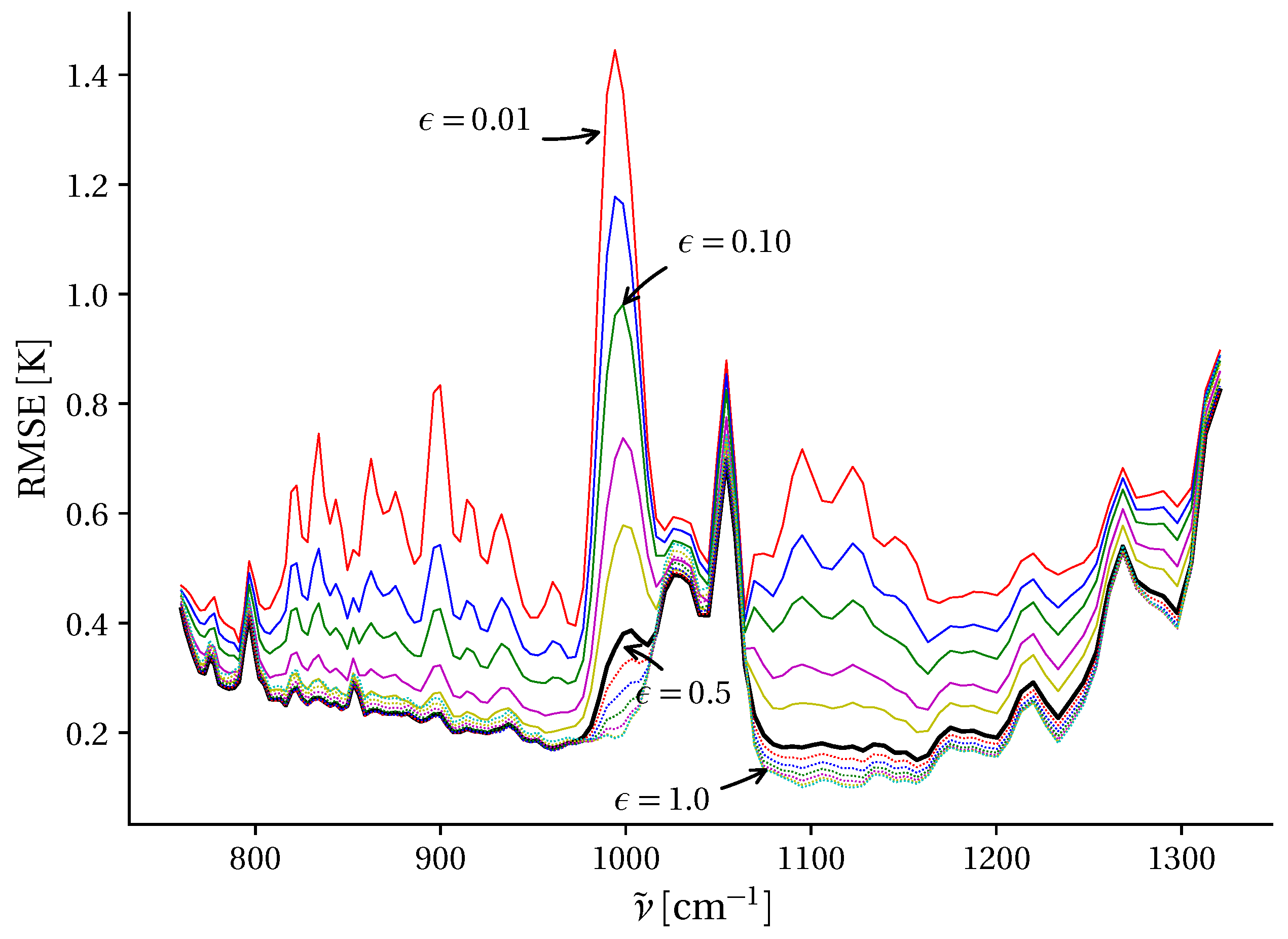
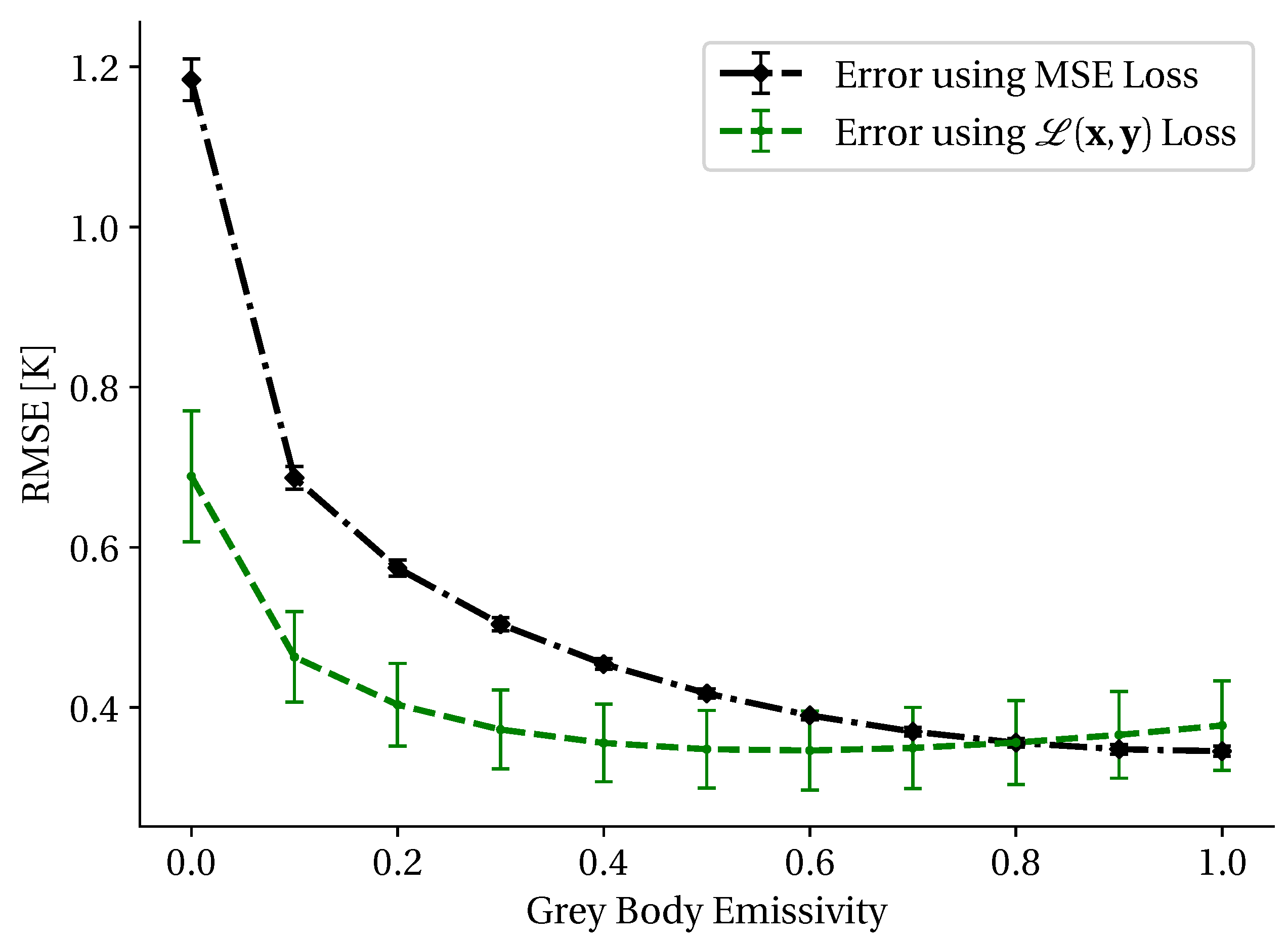
3.2. At-Sensor Loss Constraint

The same SAE architecture used to create Figure 7 is used again in this analysis where we evaluate the utility of the loss function in Equation (11). To compare the MSE against our new loss function, two identical networks were trained. Specifically, each network was initialized with the same weights and samples presented in identical order, where the only difference between the networks is in the loss calculation. Both networks use 5 components in the latent space for dimension-reduction to demonstrate differing loss characteristics for a particular network configuration. As shown in Figure 8, the physics-based loss function provides lower reconstruction error for reflective materials ( ϵ ( λ ) < 0.5 ) . This is the designed behavior of the loss function since the at-sensor radiance error for reflective materials increases based on the relationship shown in Equation (8). As the material emissivity trends toward one, the at-sensor radiance can be described by Equation (4), where errors are no longer multiplicative. In this regime, MSE and the physics-based loss function converge. The error bars in Figure 8 are based on random weight initialization of the networks for repeated training trials. MSE shows significantly less variance across repeated training but is unable to reach the lower RMSE values for reflective materials observed with the physics-based loss function. MSE outperforms the physics-based loss function for emissive materials since the reconstruction problem no longer benefits from this additional information and inhibits the model training process.

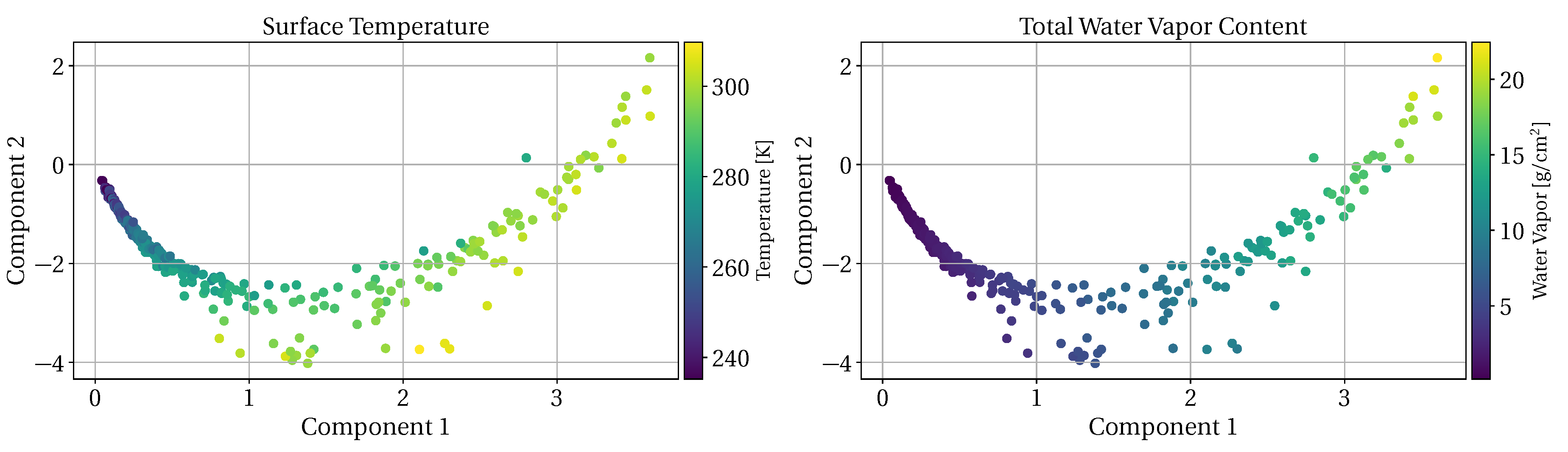
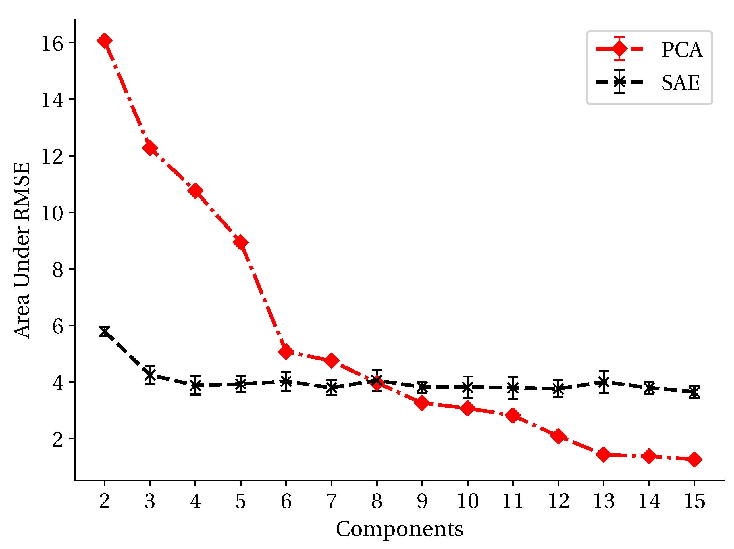
3.3. Dimension-Reduction Performance

Using the same SAE structure discussed in Section 3.1, the augmented training data and the physics-based loss function, the number of components were adjusted to compare dimension-reduction performance. Rather than creating plots similar to Figure 7 for each component configuration, the area under the RMSE curve was calculated (smaller is better), creating the plot shown in Figure 9. When the area under the curve is similar for multiple methods, we cannot determine which method is better without further analysis. This is because the individual curves demonstrate different performance characteristics for emissive and reflective materials. For example, we cannot say which method is best when using 8 components without also considering the material emissivity.
From Figure 9, it is clear lower reconstruction error can be achieved with the SAE when using a low number of components. While PCA can achieve overall lower error with greater than 8 components, this is not ideal for sampling the low-dimensional space as additional components complicate the sampling process. For the SAE model, 4 components is adequate for reconstructing the data, when considering the 176 test samples used to create these results.

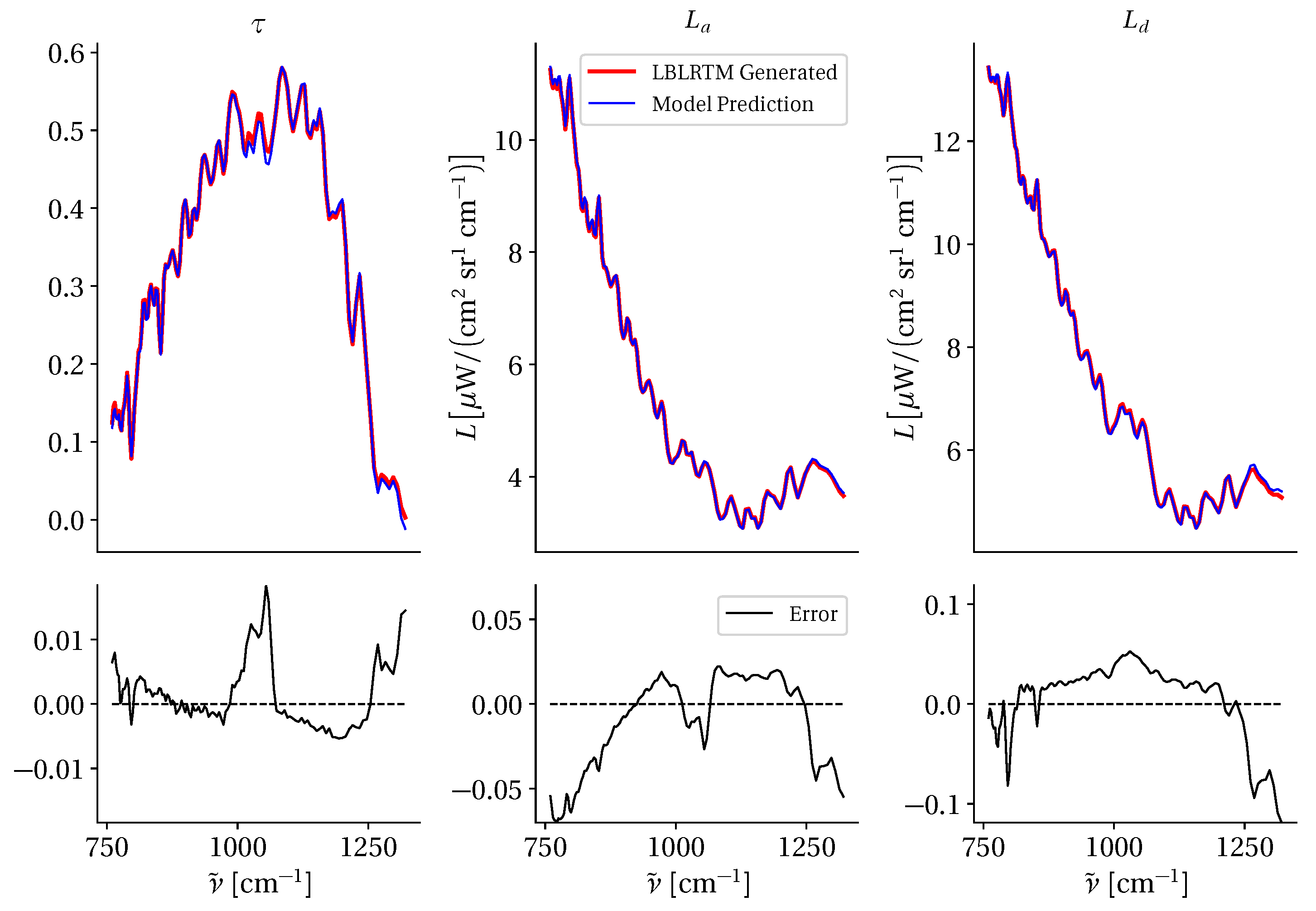
3.4. Radiative Transfer Modeling

The low-dimensional representations created by PCA and SAE can be used for efficient radiative transfer modeling by mapping TIGR atmospheric measurements to the encoder-predicted latent components. This mapping is more difficult if diverse atmospheric conditions are closely grouped in the latent space, or similarly, if small deviations in the latent space create large TUD vector differences. The same metrics used for developing the dimension-reduction methods are also used to compare RT models as we are primarily concerned with at-sensor radiance reconstruction error across a range of material emissivities.
The 66 pressure level measurements for air temperature, water content and ozone interpolated from the TIGR database are concatenated together forming a 198-dimensional input vector for latent space prediction. A two layer, fully connected neural network (58–29) is used to map the atmospheric measurement vector to the latent space. This network uses ReLU activation functions, a learning rate of 0.001, and a batch size of 16. This network configuration was identified by performing a hyperparameter sweep across number of layers, nodes per layer, activation functions, batch sizes, and learning rates resulting in over 1400 model comparisons. The atmospheric measurements were z-score standardized by feature and the latent space components were normalized between 0 and 1. This network configuration was used for the 6-component PCA model and the 4-component SAE model. The 6-component PCA model was selected for this analysis because of the large reduction in RMSE error from 5 to 6 components. In both cases, the network was trained for 500 epochs with validation and training loss stabilizing between 200 and 300 epochs. This model configuration was found by performing a hyperparameter sweep for the PCA model and identifying the configuration with minimum validation set at-sensor reconstruction error for a range of emissivity values. The sampling network weights were updated based on latent space component prediction errors with SAE using standard MSE loss. For sampling the PCA latent space, weighted MSE loss was used as outlined in Equation (12).
The resulting RMSE for each RT model is shown in Figure 10 where the RT model derived from the SAE decoder has the lowest error across all emissivity values. The artificial neural network (ANN) model results shown in Figure 10 represent a baseline approach where an end-to-end neural network was trained with the same network configuration as the SAE RT model (198-58-29-4-15-40-384) using MSE for the model loss function. The performance difference between the SAE RT model and the ANN model highlight the advantages of first using an AE to initially fit network weights before training the RT model. Initially training the SAE weights clusters similar atmospheric conditions together, limiting the impact of RT model sampling errors, improving overall RT model performance. Additionally, the at-sensor radiance loss function used in the SAE approach significantly improves model performance for reflective materials. Without the at-sensor radiance loss function or the weight initialization imposed by training an AE model, the ANN model is unable to reconstruct TUD vectors with the accuracy of the SAE RT model.
The SAE RT model was trained by first fitting encoder and decoder networks to minimize at-sensor radiance reconstruction error, following by training a small sampling network to correctly predict latent components. This training methodology did not allow updates to the decoder network after training of the sampling network. The SAE RT Tuned model result shown in Figure 10, has the same configuration as the SAE RT model, but the decoder weights were also updated after the sampling network training converged. This final training step used the same physics-based loss function used for the initial SAE training, improving reconstruction performance for reflective emissivity values. Since the previous training steps had already created weight matrices resulting in high performance, only small changes were needed to further reduce reconstruction error.
Additionally, the 15 component PCA model results are shown. In this case, even higher RMSE error is observed since correctly sampling the 15 components is a more complex task. While the 15 component PCA model has the lowest reconstruction error during the TUD reconstruction training phase, the added complexity in latent space fitting limits the utility of this model. In all cases the highest errors are observed for reflective materials since errors in transmittance and downwelling radiance are multiplicative in this region.
Considering only the SAE RT Tuned model, the at-sensor radiance RMSE as a function of wavenumber and emissivity is shown in Figure 11. These results are the average RMSE for the 176 test TIGR samples at each emissivity level. For emissive materials, RT model errors are below 0.5 K for most bands. The ozone absorption bands between 1050 and 1100 cm 1 lead to larger errors because of limited transmittance in this domain of the spectrum resulting in large deviations in the at-sensor radiance. The challenge of correctly identifying a TUD vector for reflective materials is seen by the high RMSE for ϵ = 0.01 in Figure 11. While these errors appear large on the scale shown in Figure 11, these errors are significantly larger using other models based on the results for ϵ = 0 in Figure 10.
Based on the results shown in Figure 11, the SAE-based RT model can estimate TUD vectors with errors below 0.5 K for most spectral bands and a range of emissivity values. These generated TUD vectors are useful for estimating surface leaving radiance described in Equation (3) if estimates of atmospheric conditions can be provided.
Also, the RT model can be used to quickly estimate TUD vectors. The RT model developed here is approximately 15 times faster than the correlated-k method. On average, a single TUD vector can be predicted in 0.1 s; however, this increase in performance is amplified when considering batch processing as multiple TUD predictions can be performed in parallel. By reducing TUD prediction time, this method is useful for quickly generating augmented representations of emissivity profiles based on multiple atmospheric state vectors. The data was constructed such that this method could be used for the Mako LWIR hyperspectral sensor; however, resampling of the high-resolution LBLRTM data can be performed for other sensors.

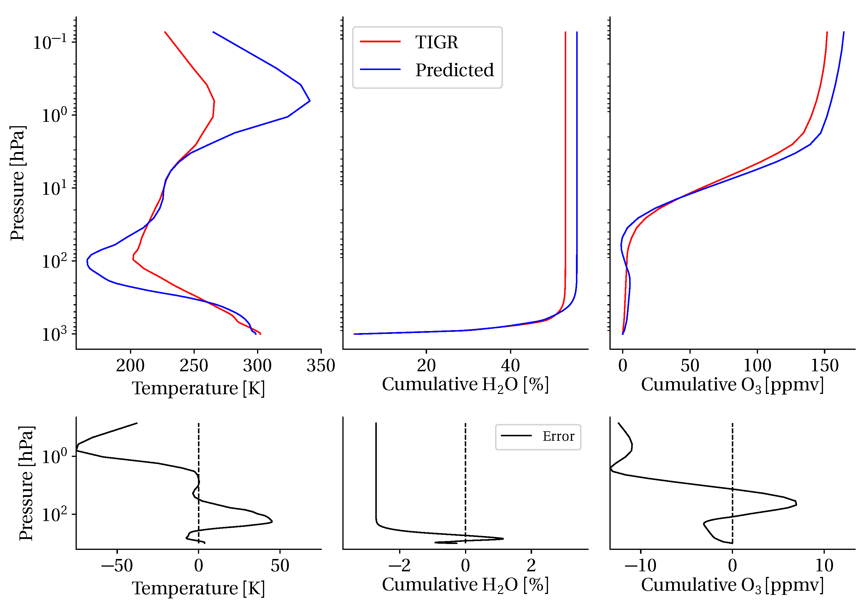
3.5. Atmospheric Measurement Estimation

Finally, we consider estimation of the most likely atmospheric measurements for a given TUD vector using the formulated RT model. Instead of propagating inputs forward through the RT model, this section considers estimation of the model’s inputs for a given output. Since the RT model is composed of a sampling network (atmospheric measurements to latent components) and a decoder network (latent components to TUD vectors) the estimation problem can be partitioned into two steps.
First, the latent space components are identified that correspond to the TUD vector. Since the latent space only consists of 4 components, finding these 4 components using an optimizer takes little time and results in predicted TUD vectors closely matching the given TUD vector. This optimization is performed with respect to the decoder network of the RT model. As an example of this process, we select a TUD vector with a 50th percentile reconstruction error from the test data set. Figure 12 shows the LBLRTM generated TUD components and the predicted TUD from optimizing the 4 latent components.
After identifying the latent components, inputs to the sampling network (atmospheric measurements to latent components) must be optimized to identify measurements that will produce the estimated latent components. Unfortunately, the input measurement vector contains 198 values (temperature, water content and ozone at 66 pressure levels) and optimizing this large number of values for 4 components is a time-consuming and difficult task.
To make this problem more tractable, a PCA transform was applied to the training data atmospheric measurements. Using 10 components to represent the atmospheric measurements captures 90% of data variance and simplifies the optimization problem as only 10 values must be optimized to predict the 4 latent components. For the same TUD vector used in Figure 12, the result of the atmospheric measurement estimation process is shown in Figure 13. Interestingly, the largest errors occur at high altitudes, where deviations in these measurements have less impact due to lower air density.
The results shown in Figure 12 and Figure 13 are for a single TUD vector. This process was repeated for all TUD vectors in the test data set to determine overall performance metrics. Errors between predicted temperature and water content measurements and the corresponding TIGR atmospheric measurements are weighted by the density at the discrete pressure levels as errors at high altitudes will have a lower impact on the TUD vector prediction. For all 176 test set TUD vectors, we observe an average error of 2.61 K for predicted temperature profiles and 0.45 cumulative H 2 O % for predicted water content profiles. For ozone measurements, an atmospheric density weighting was not applied. The observed average error for ozone measurement estimation was 0.79 ppmv.
Overall, the goal of the RT model is to predict TUD vectors, based on known or estimated atmospheric measurements. By showing the model’s ability to estimate atmospheric measurements from a given TUD vector (inverse problem), we have demonstrated the utility of low-dimension representations of the TUD vectors. Additionally, since the latent space clusters similar atmospheric conditions together (latent-space-similarity), an ensemble of likely atmospheric measurements can be generated for a given TUD by applying small deviations to latent components.

4. Conclusions

This study has leveraged SAEs with a novel physics-based loss function to reduce TUD vector dimensionality such that fast and effective LWIR RT models could be constructed by sampling the low-dimensional TUD representation. By using an AE pre-training step, the low-dimensional TUD representation clustered similar atmospheric conditions together reducing sampling errors. Additionally, the pre-training step verified that small deviations in the low-dimensional TUD representation corresponded to small deviations in the high-dimensional TUD vector. These approaches were shown to reconstruct at-sensor radiance with errors below 0.5 K for most emissivity values.
The dimension-reduction results used real atmospheric measurements from the TIGR database and augmented data derived from this same database. Using augmented atmospheric measurements improved both PCA and SAE performance for a range of material emissivities. PCA was shown to reconstruct data with lower error than the SAE when using beyond 8 components. The SAE performance did not improve significantly when using more than 4 components, demonstrating adequate capacity for the augmented TIGR data.
Sampling the low-dimensional representations created by these methods highlighted significant differences in TUD reconstruction. This study found the SAE latent space easier to sample, resulting in lower RT model errors. Additionally, training the entire RT model after pre-training the sampling network and decoder networks improved RT performance. The RT model was further explored to identify the most likely atmospheric measurements for a given TUD vector. This analysis revealed that RT model inputs could easily be optimized resulting in predicted atmospheric measurements with some agreement to the TIGR measurements. While this was not the goal of this work, we will explore the utility and limitations of SAEs in the inverse problem of estimating atmospheric conditions from spectral measurements.
Optimizing the latent components for a particular TUD vector is a straightforward process; however, no known physical quantities are directly correlated with these components. No constraints were placed on the formulation of this latent space other than the overall network loss function. This unconstrained representation creates a disentanglement problem limiting the utility of the SAE as a generative model when limited atmospheric information is available. Future work in this area will consider additional constraints on the latent space to improve upon this disentanglement problem, offering a means for creating TUD vectors with properties representative of specific atmospheric conditions. Specifically, if complete atmospheric measurements are not available, this analysis will determine what information is required to predict the most likely TUD vector using a small number of components. Methods such as Variational AEs, multi-modal AEs and Generative Adversarial Networks coupled with physical constraints will be investigated toward this goal.

Author Contributions

All coauthors contributed to the research methodology and manuscript. N.W. led the research investigation, wrote the first draft, and developed all the dimension-reduction, analysis, and visualization code. K.C.G. and B.B. provided mentorship and ideas related to the blending of physics principles and machine learning in the dimension-reduction approach.

Funding

This research was supported by Jacob Martin at Air Force Research Laboratory through the effort “Developing Physics-Based Machine Learning Algorithms to Exploit Hyperspectral Imagery.”

Acknowledgments

The views and conclusions contained in this document are those of the authors and should not be interpreted as representing the official policies, either expressed or implied, of the United States Air Force or the U.S. Government.

Conflicts of Interest

The authors declare no conflict of interest.

References

  1. Hall, J.L.; Boucher, R.H.; Buckland, K.N.; Gutierrez, D.J.; Keim, E.R.; Tratt, D.M.; Warren, D.W. Mako airborne thermal infrared imaging spectrometer: Performance update. In Proceedings of the Imaging Spectrometry XXI, San Diego, CA, USA, 28 August–1 September 2016; International Society for Optics and Photonics; Volume 9976. [Google Scholar]
  2. Goetz, A.F.; Vane, G.; Solomon, J.E.; Rock, B.N. Imaging spectrometry for earth remote sensing. Science 1985, 228, 1147–1153. [Google Scholar] [CrossRef]
  3. Eismann, M.T. Hyperspectral Remote Sensing; SPIE: Bellingham, WA, USA, 2012. [Google Scholar]
  4. Manolakis, D.G.; Lockwood, R.B.; Cooley, T.W. Hyperspectral Imaging Remote Sensing: Physics, Sensors, and Algorithms; Cambridge University Press: Cambridge, UK, 2016. [Google Scholar]
  5. Gao, B.C.; Montes, M.J.; Davis, C.O.; Goetz, A.F. Atmospheric correction algorithms for hyperspectral remote sensing data of land and ocean. Remote Sens. Environ. 2009, 113, S17–S24. [Google Scholar] [CrossRef]
  6. Liu, X.; Smith, W.L.; Zhou, D.K.; Larar, A. Principal component-based radiative transfer model for hyperspectral sensors: Theoretical concept. Appl. Opt. 2006, 45, 201–209. [Google Scholar] [CrossRef] [PubMed]
  7. Kopparla, P.; Natraj, V.; Spurr, R.; Shia, R.L.; Crisp, D.; Yung, Y.L. A fast and accurate PCA based radiative transfer model: Extension to the broadband shortwave region. J. Quantit. Spectrosc. Radiat. Transf. 2016, 173, 65–71. [Google Scholar] [CrossRef]
  8. Goody, R.; West, R.; Chen, L.; Crisp, D. The correlated-k method for radiation calculations in nonhomogeneous atmospheres. J. Quantit. Spectrosc. Radiat. Transf. 1989, 42, 539–550. [Google Scholar] [CrossRef]
  9. Natraj, V.; Jiang, X.; Shia, R.l.; Huang, X.; Margolis, J.S.; Yung, Y.L. Application of principal component analysis to high spectral resolution radiative transfer: A case study of the O2 A band. J. Quantit. Spectrosc. Radiat. Transf. 2005, 95, 539–556. [Google Scholar] [CrossRef]
  10. Matricardi, M. A principal component based version of the RTTOV fast radiative transfer model. Q. J. R. Meteorol. Soc. 2010, 136, 1823–1835. [Google Scholar] [CrossRef]
  11. Aguila, A.; Efremenko, D.S.; Molina Garcia, V.; Xu, J. Analysis of Two Dimensionality Reduction Techniques for Fast Simulation of the Spectral Radiances in the Hartley-Huggins Band. Atmosphere 2019, 10, 142. [Google Scholar] [CrossRef]
  12. Young, S.J.; Johnson, B.R.; Hackwell, J.A. An in-scene method for atmospheric compensation of thermal hyperspectral data. J. Geophys. Res. Atmos. 2002, 107, ACH-14. [Google Scholar] [CrossRef]
  13. Gu, D.; Gillespie, A.R.; Kahle, A.B.; Palluconi, F.D. Autonomous atmospheric compensation (AAC) of high resolution hyperspectral thermal infrared remote-sensing imagery. IEEE Trans. Geosci. Remote Sens. 2000, 38, 2557–2570. [Google Scholar]
  14. Borel, C.C. ARTEMISS—An algorithm to retrieve temperature and emissivity from hyper-spectral thermal image data. In Proceedings of the 28th Annual GOMACTech Conference, Hyperspectral Imaging Session, Tampa, FL, USA, 31 March–3 April 2003; Volume 31, pp. 1–4. [Google Scholar]
  15. Chedin, A.; Scott, N.; Wahiche, C.; Moulinier, P. The improved initialization inversion method: A high resolution physical method for temperature retrievals from satellites of the TIROS-N series. J. Clim. Appl. Meteorol. 1985, 24, 128–143. [Google Scholar] [CrossRef]
  16. Chevallier, F.; Chéruy, F.; Scott, N.; Chédin, A. A neural network approach for a fast and accurate computation of a longwave radiative budget. J. Clim. Appl. Meteorol. 1998, 37, 1385–1397. [Google Scholar] [CrossRef]
  17. Acito, N.; Diani, M.; Corsini, G. Coupled subspace-based atmospheric compensation of LWIR hyperspectral data. IEEE Trans. Geosci. Remote Sens. 2019. [Google Scholar] [CrossRef]
  18. Martin, J.A. Target detection using artificial neural networks on LWIR hyperspectral imagery. In Algorithms and Technologies for Multispectral, Hyperspectral, and Ultraspectral Imagery XXIV; International Society for Optics and Photonics: Bellingham, WA, USA, 2018; Volume 10644. [Google Scholar] [CrossRef]
  19. Warren, D.; Boucher, R.; Gutierrez, D.; Keim, E.; Sivjee, M. MAKO: A high-performance, airborne imaging spectrometer for the long-wave infrared. In Imaging Spectrometry XV; International Society for Optics and Photonics: Bellingham, WA, USA, 2010; Volume 7812, p. 78120N. [Google Scholar] [CrossRef]
  20. Friedman, J.; Hastie, T.; Tibshirani, R. The Elements of Statistical Learning; Springer: New York, NY, USA, 2001; Volume 1. [Google Scholar]
  21. Hinton, G.E.; Salakhutdinov, R.R. Reducing the dimensionality of data with neural networks. Science 2006, 313, 504–507. [Google Scholar] [CrossRef] [PubMed]
  22. Nair, V.; Hinton, G.E. Rectified linear units improve restricted boltzmann machines. In Proceedings of the 27th International Conference on Machine Learning (ICML-10), Haifa, Israel, 21–24 June 2010; pp. 807–814. [Google Scholar]
  23. Maas, A.L.; Hannun, A.Y.; Ng, A.Y. Rectifier nonlinearities improve neural network acoustic models. In Proceedings of the ICML Workshop on Deep Learning for Audio, Speech and Language Processing, Atlanta, GA, USA, 16–21 June 2013. [Google Scholar]
  24. Chen, Y.; Lin, Z.; Zhao, X.; Wang, G.; Gu, Y. Deep learning-based classification of hyperspectral data. IEEE J. Sel. Top. Appl. Earth Obs. Remote Sens. 2014, 7, 2094–2107. [Google Scholar] [CrossRef]
Figure 1. The high-resolution LBLRTM transmittance, upwelling and downwelling vectors are shown with their downsampled counterparts for the Mako LWIR sensor. The downsampled vectors are the data used in the remainder of this study.
Remotesensing 11 01866 g001
Figure 2. An example AE model where the TUD vectors are compressed through one or more encoder layers to a low-dimensional latent space. The decoder transforms the low-dimensional latent space back to the original TUD vector.
Remotesensing 11 01866 g002
Figure 3. The first two principal components using a 6 component PCA model with the augmented TIGR data. Hot, humid atmospheric conditions vary with component 1 and 2 while cold, dry atmospheres are more dependent on component 2.
Remotesensing 11 01866 g003
Figure 4. Autoencoder latent space when trained using 2 components. The points are scattered throughout the latent space with an overall clustering of similar atmospheric conditions. Both components appear dependent on surface temperature. Component 1 also appears more dependent on total water content versus component 2.
Remotesensing 11 01866 g004
Figure 5. The RT model is created by first creating a low-dimensional representation of the TUD vectors with acceptable at-sensor radiance reconstruction errors. The latent space and decoder parameters are locked, and a sampling model is fit to correctly identify the low-dimensional components to map atmospheric measurements to their corresponding TUD vectors. This diagram is specific for the SAE approach, but the encoder and decoder can be replaced with equivalent PCA transformations.
Remotesensing 11 01866 g005
Figure 6. Generated atmospheric measurements based on sampled PCA components from the GMM.
Remotesensing 11 01866 g006
Figure 7. Dimension-reduction techniques show improved results when using the augmented TIGR data. All models reduce the input data to 5 components in this plot; however, the number of components is an additional hyperparameter that will be considered later.
Remotesensing 11 01866 g007
Figure 8. Comparison of SAE performance when using strictly MSE loss or the loss function described in Equation (11). Updating the model using information from the at-sensor radiance error improves reconstruction performance for reflective materials. The error bars represent the performance standard deviation when training multiple networks with identical architectures and random weight initialization.
Remotesensing 11 01866 g008
Figure 9. Varying the number of latent components and calculating the area under the RMSE curve shown in Figure 8 shows how many components are necessary to reconstruct the TIGR data. Results are plotted for the validation set consisting of 158 samples using the augmented data for training and the loss function outlined in Equation (11) for SAE training. The PCA error bars correspond to performance standard deviation when using 5-fold cross-validation. The SAE errors bars show the performance standard deviation when random weight initialization is used.
Remotesensing 11 01866 g009
Figure 10. The performance of the RT models is shown as a function of emissivity where it is clear the SAE derived RT models create a latent space that is easier to sample with a small neural network. In all cases performance improves as materials become more emissive since downwelling radiance plays a less significant role in these cases. The 15 component PCA model is also shown, where sampling the 15 components correctly becomes a complex problem resulting in lower overall performance.
Remotesensing 11 01866 g010
Figure 11. The at-sensor radiance RMSE RT model errors for 176 test TIGR samples as a function of surface emissivity expressed in spectral brightness temperature. Model errors decrease with increasing emissivity, consistent with the findings in Figure 10.
Remotesensing 11 01866 g011
Figure 12. The top 3 panels are the predicted TUD components plotted against the LBLRTM generated TUD components. The predicted TUD components were generated by optimizing the 4 latent components. The bottom 3 panels are the TUD component residual curves, showing low error across most spectral channels.
Remotesensing 11 01866 g012
Figure 13. Predicted atmospheric measurements compared to the TIGR atmospheric measurements. The predicted atmospheric measurements will produce a close match to a given TUD vector but do show some deviations from the original TIGR measurement, specifically at high altitudes. Fortunately, high altitude error has less impact on the at-sensor radiance error because of lower air density.
Remotesensing 11 01866 g013

