The Effect of Droughts on Vegetation Condition in Germany: An Analysis Based on Two Decades of Satellite Earth Observation Time Series and Crop Yield Statistics


Abstract
1. Introduction
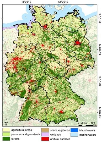
2. Study Region
3. Materials and Methods
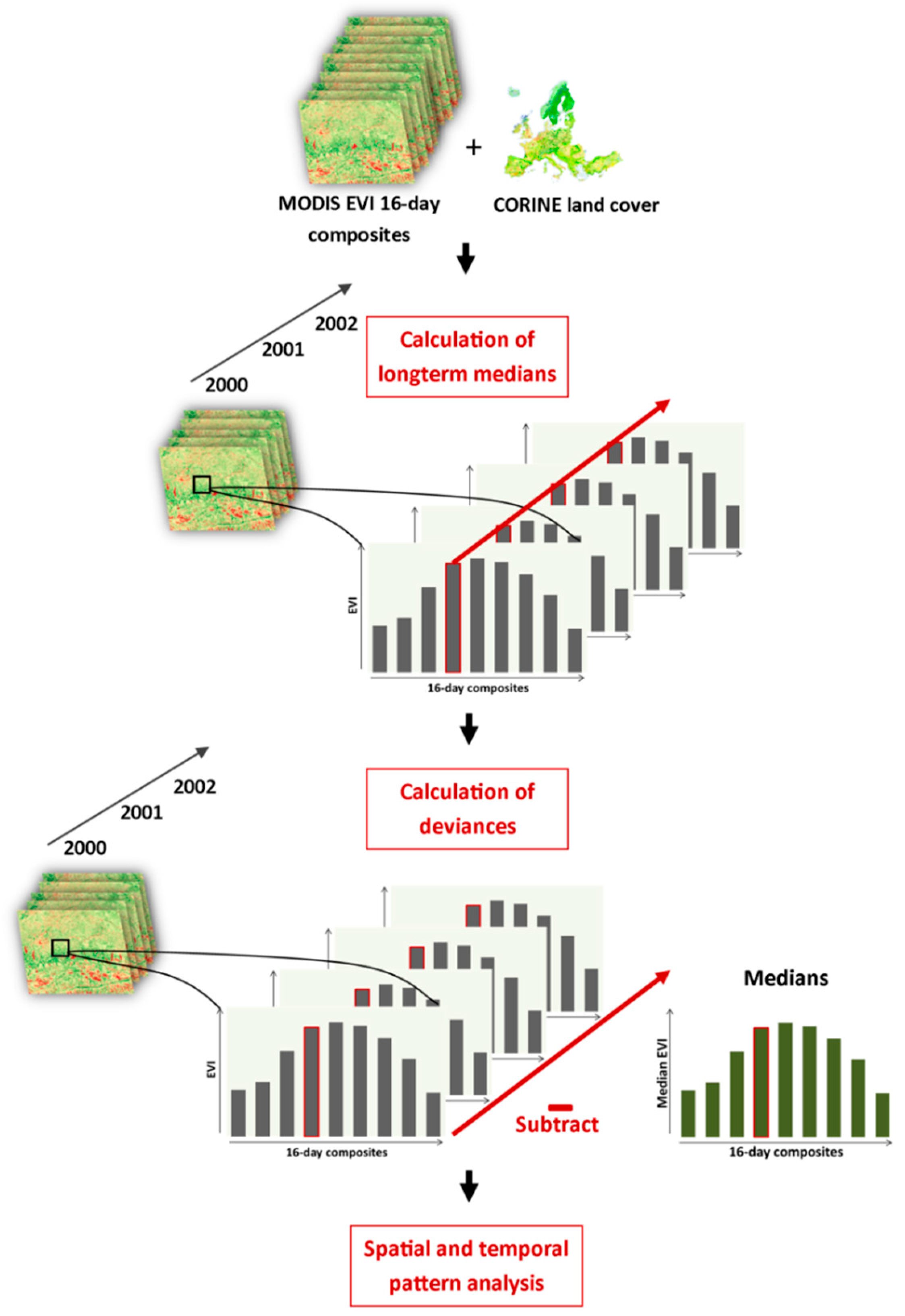
3.1. Input Data
3.2. Data Processing and Analysis
4. Results
4.1. Multi-Annual Temporal Patterns of Vegetation Anomalies
4.2. Spatial Patterns of Vegetation Anomalies
4.3. Comparison with Yield Statistics
5. Discussion
5.1. The Most Extreme Years of the Study Period
5.2. Comparison of EVI Anomalies with Weather Data and Crop Yields
5.2.1. The Years 2003 and 2018
5.2.2. EVI Deviances and Their Drivers in Other Years
5.3. Effects for Different Land Cover Types
5.4. Suitability of the Methods Used
6. Conclusions
Supplementary Materials
Author Contributions
Funding
Acknowledgments
Conflicts of Interest
References
- Masante, D.; Vogt, J. Drought in Central-Northern Europe—August 2018. 2018. Available online: http://edo.jrc.ec.europa.eu/documents/news/EDODroughtNews201808_Central_North_Europe.pdf (accessed on 14 June 2019).
- IPCC. Global Warming of 1.5 °C; An IPCC Special Report on the Impacts of Global Warming of 1.5 °C above Pre-Industrial Levels and Related Global Greenhouse Gas Emission Pathways, in the Context of Strengthening the Global Response to the Threat of Climate Change, Sustainable Development, and Efforts to Eradicate Poverty; 2018; Available online: https://www.ipcc.ch/sr15/ (accessed on 26 July 2019).
- IPCC. Climate Change 2013: The Physical Science Basis; Contribution of Working Group I to the Fifth Assessment Report of the Intergovernmental Panel on Climate Change; 2013; Available online: https://www.ipcc.ch/report/ar5/wg1/ (accessed on 26 July 2019).
- Suarez-Gutierrez, L.; Li, C.; Müller, W.A.; Marotzke, J. Internal variability in European summer temperatures at 1.5 °C and 2 °C of global warming. Environ. Res. Lett. 2018, 13, 064026. [Google Scholar] [CrossRef]
- Spinoni, J.; Vogt, J.V.; Naumann, G.; Barbosa, P.; Dosio, A. Will drought events become more frequent and severe in Europe? Int. J. Climatol. 2018, 38, 1718–1736. [Google Scholar] [CrossRef]
- Samaniego, L.; Thober, S.; Kumar, R.; Wanders, N.; Rakovec, O.; Pan, M.; Zink, M.; Sheffield, J.; Wood, E.F.; Marx, A. Anthropogenic warming exacerbates European soil moisture droughts. Nat. Clim. Chang. 2018, 8, 421. [Google Scholar] [CrossRef]
- Grillakis, M.G. Increase in severe and extreme soil moisture droughts for Europe under climate change. Sci. Total Environ. 2019, 660, 1245–1255. [Google Scholar] [CrossRef] [PubMed]
- De Bono, A.; Guiliani, G.; Kluser, S.; Peduzzi, P. Impacts of Summer 2003 Heat Wave in Europe. 2018. Available online: https://www.unisdr.org/files/1145_ewheatwave.en.pdf (accessed on 14 June 2019).
- Crausbay, S.D.; Ramirez, A.R.; Carter, S.L.; Cross, M.S.; Hall, K.R.; Bathke, D.J.; Betancourt, J.L.; Colt, S.; Cravens, A.E.; Dalton, M.S.; et al. Defining Ecological Drought for the Twenty-First Century. Bull. Am. Meteorol. Soc. 2017, 98, 2543–2550. [Google Scholar] [CrossRef]
- Bastos, A.; Gouveia, C.M.; Trigo, R.M.; Running, S.W. Analysing the spatio-temporal impacts of the 2003 and 2010 extreme heatwaves on plant productivity in Europe. Biogeosciences 2014, 11, 3421–3435. [Google Scholar] [CrossRef]
- Gammans, M.; Mérel, P.; Ortiz-Bobea, A. Negative impacts of climate change on cereal yields: Statistical evidence from France. Environ. Res. Lett. 2017, 12, 054007. [Google Scholar] [CrossRef]
- Obermeier, W.A.; Lehnert, L.W.; Ivanov, M.A.; Luterbacher, J.; Bendix, J. Reduced Summer Aboveground Productivity in Temperate C3 Grasslands under Future Climate Regimes. Earth’s Future 2018, 6, 716–729. [Google Scholar] [CrossRef]
- Imbery, F.; Friedrich, K.; Koppe, C.; Janssen, W.; Pfeifroth, U.; Daßler, J.; Bissolli, P. 2018 wärmster Sommer im Norden und Osten Deutschlands. 2018. Available online: https://www.dwd.de/DE/leistungen/besondereereignisse/temperatur/20180906_waermstersommer_nordenosten2018.html (accessed on 14 December 2018).
- Hänsel, S.; Ustrnul, Z.; Lupikasza, E.; Skalak, P. Assessing seasonal drought variations and trends over Central Europe. Adv. Water Resour. 2019, 127, 53–75. [Google Scholar] [CrossRef]
- BMEL. Vereinbarung für das Dürrehilfsprogramm Ist Jetzt von allen Teilnehmenden Bundesländern Unterzeichnet. 2018. Available online: https://www.bmel.de/SharedDocs/Pressemitteilungen/2018/155-Vereinbarung_Duerrehilfsprogramm.html (accessed on 14 June 2019).
- Vicente-Serrano, S.M. Evaluating the Impact of Drought Using Remote Sensing in a Mediterranean, Semi-arid Region. Nat. Hazards 2007, 40, 173–208. [Google Scholar] [CrossRef]
- Winkler, K.; Gessner, U.; Hochschild, V. Identifying Droughts Affecting Agriculture in Africa Based on Remote Sensing Time Series between 2000–2016: Rainfall Anomalies and Vegetation Condition in the Context of ENSO. Remote Sens. 2017, 9, 831. [Google Scholar] [CrossRef]
- Gouveia, C.M.; Trigo, R.M.; Beguería, S.; Vicente-Serrano, S.M. Drought impacts on vegetation activity in the Mediterranean region: An assessment using remote sensing data and multi-scale drought indicators. Glob. Planet. Chang. 2017, 151, 15–27. [Google Scholar] [CrossRef]
- Zscheischler, J.; Mahecha, M.D.; Harmeling, S.; Reichstein, M. Detection and attribution of large spatiotemporal extreme events in Earth observation data. Ecol. Inform. 2013, 15, 66–73. [Google Scholar] [CrossRef]
- Yu, Z.; Wang, J.; Liu, S.; Rentch, J.S.; Sun, P.; Lu, C. Global gross primary productivity and water use efficiency changes under drought stress. Environ. Res. Lett. 2017, 12, 014016. [Google Scholar] [CrossRef]
- Vicente-Serrano, S.M.; Gouveia, C.; Camarero, J.J.; Beguería, S.; Trigo, R.; López-Moreno, J.I.; Azorín-Molina, C.; Pasho, E.; Lorenzo-Lacruz, J.; Revuelto, J.; et al. Response of vegetation to drought time-scales across global land biomes. Proc. Natl. Acad. Sci. USA 2013, 110, 52–57. [Google Scholar] [CrossRef] [PubMed]
- Ahmadi, B.; Ahmadalipour, A.; Tootle, G.; Moradkhani, H. Remote sensing of water use efficiency and terrestrial drought recovery across the contiguous united states. Remote Sens. 2019, 11, 731. [Google Scholar] [CrossRef]
- Ivits, E.; Horion, S.; Fensholt, R.; Cherlet, M. Drought footprint on E uropean ecosystems between 1999 and 2010 assessed by remotely sensed vegetation phenology and productivity. Glob. Chang. Biol. 2014, 20, 581–593. [Google Scholar] [CrossRef] [PubMed]
- Le Page, M.; Zribi, M. Analysis and predictability of drought in Northwest Africa using optical and microwave satellite remote sensing products. Sci. Rep. 2019, 9, 1466. [Google Scholar] [CrossRef] [PubMed]
- Reichstein, M.; Ciais, P.; Papale, D.; Valentini, R.; Running, S.; Viovy, N.; Cramer, W.; Granier, A.; Ogee, J.; Allard, V.; et al. Reduction of ecosystem productivity and respiration during the European summer 2003 climate anomaly: A joint flux tower, remote sensing and modelling analysis. Glob. Chang. Biol. 2007, 13, 634–651. [Google Scholar] [CrossRef]
- Vicca, S.; Balzarolo, M.; Filella, I.; Granier, A.; Herbst, M.; Knohl, A.; Longdoz, B.; Mund, M.; Nagy, Z.; Pintér, K.; et al. Remotely-sensed detection of effects of extreme droughts on gross primary production. Sci. Rep. 2016, 6, 28269. [Google Scholar] [CrossRef] [PubMed]
- Nicolai-Shaw, N.; Zscheischler, J.; Hirschi, M.; Gudmundsson, L.; Seneviratne, S.I. A drought event composite analysis using satellite remote-sensing based soil moisture. Remote Sens. Environ. 2017, 203, 216–225. [Google Scholar] [CrossRef]
- Zandalinas, S.I.; Mittler, R.; Balfagón, D.; Arbona, V.; Gómez-Cadenas, A. Plant adaptations to the combination of drought and high temperatures. Physiol. Plant. 2018, 162, 2–12. [Google Scholar] [CrossRef] [PubMed]
- Reichstein, M.; Bahn, M.; Ciais, P.; Frank, D.; Mahecha, M.D.; Seneviratne, S.I.; Zscheischler, J.; Beer, C.; Buchmann, N.; Frank, D.C.; et al. Climate extremes and the carbon cycle. Nature 2013, 500, 287. [Google Scholar] [CrossRef] [PubMed]
- DWD. Monthly Temperature and Precipitation Data for the States of Germany. 2018. Available online: ftp://ftp-cdc.dwd.de/pub/CDC/regional_averages_DE/monthly/ (accessed on 1 February 2019).
- Destatis. Genesis-Online: Datenlizenz by-2-0. Available online: https://www-genesis.destatis.de/genesis/online/logon (accessed on 14 June 2019).
- EEA. CORINE Land Monitoring Service 2012. 2012. Available online: https://land.copernicus.eu/pan-european/corine-land-cover (accessed on 9 November 2018).
- Didan, K. MOD13Q1 MODIS/Terra Vegetation Indices 16-Day L3 Global 250m SIN Grid V006 [Data set]. NASA EOSDIS Land Processes DAAC. 2015. Available online: https://lpdaac.usgs.gov/products/mod13q1v006/ (accessed on 29 July 2019).
- Gorelick, N.; Hancher, M.; Dixon, M.; Ilyushchenko, S.; Thau, D.; Moore, R. Google Earth Engine: Planetary-scale geospatial analysis for everyone. Remote Sens. Environ. 2017, 202, 18–27. [Google Scholar] [CrossRef]
- Kornhuber, K.; Osprey, S.; Coumou, D.; Petri, S.; Petoukhov, V.; Rahmstorf, S.; Gray, L. Extreme weather events in early summer 2018 connected by a recurrent hemispheric wave-7 pattern. Environ. Res. Lett. 2019, 14, 054002. [Google Scholar] [CrossRef]
- Imbery, F.; Friedrich, K.; Fleckenstein, R.; Kaspar, F.; Ziese, M.; Fildebrandt, J.; Schube, C. Mai 2018: Zweiter Monatlicher Temperaturrekord in Folge, Regional mit Dürren und Starkniederschlägen. 2018. Available online: https://www.dwd.de/DE/leistungen/besondereereignisse/temperatur/20180604_bericht_mai2018.pdf (accessed on 17 June 2019).
- Müller-Westermeier, G.; Riecke, W. Die Witterung in Deutschland. In Klimastatusbericht 2003; DWD, Ed.; DWD (Deutscher Wetterdienst): Offenbach, Germany, 2004; pp. 71–78. [Google Scholar]
- Rebetez, M.; Mayer, H.; Dupont, O.; Schindler, D.; Gartner, K.; Kropp, J.P.; Menzel, A. Heat and drought 2003 in Europe: A climate synthesis. Ann. For. Sci. 2006, 63, 569–577. [Google Scholar] [CrossRef]
- Laaha, G.; Gauster, T.; Tallaksen, L.M.; Vidal, J.-P.; Stahl, K.; Prudhomme, C.; Heudorfer, B.; Vlnas, R.; Ionita, M.; van Lanen, H.A.J.; et al. The European 2015 drought from a hydrological perspective. Hydrol. Earth Syst. Sci. 2017, 21, 3001–3024. [Google Scholar] [CrossRef]
- Matiu, M.; Ankerst, D.P.; Menzel, A. Interactions between temperature and drought in global and regional crop yield variability during 1961–2014. PLoS ONE 2017, 12, 1–23. [Google Scholar] [CrossRef]
- Müller-Westermeier, G.; Lefebvre, C.; Nitsche, H.; Riecke, W.; Zimmermann, K. Die Witterung in Deutschland 2006. In Klimastatusbericht 2006; DWD, Ed.; DWD (Deutscher Wetterdienst): Offenbach, Germany, 2007; pp. 5–27. [Google Scholar]
- Rebetez, M.; Dupont, O.; Giroud, M. An analysis of the July 2006 heatwave extent in Europe compared to the record year of 2003. Theor. Appl. Climatol. 2009, 95, 1–7. [Google Scholar] [CrossRef]
- Müller-Westermeier, G.; Lefebvre, C.; Nitsche, H.; Riecke, W.; Zimmermann, K. Die Witterung in Deutschland. In Klimastatusbericht 2007; DWD, Ed.; DWD (Deutscher Wetterdienst): Offenbach, Germany, 2008; pp. 25–49. [Google Scholar]
- Löpmeier, F.-J.; Trampf, W. Die agrarmeteorologische Situation im Jahr 2007. In Klimastatusbericht 2007; DWD, Ed.; DWD (Deutscher Wetterdienst): Offenbach, Germany, 2008; pp. 50–60. [Google Scholar]
- BMEL. Ernte 2011: Mengen und Preise. 2011. Available online: http://www.bmel-statistik.de/fileadmin/user_upload/monatsberichte/EQB-6011010-2011.pdf (accessed on 8 March 2019).
- BMEL. Ernte 2013: Mengen und Preise. 2013. Available online: https://www.bmel.de/SharedDocs/Downloads/Landwirtschaft/Markt-Statistik/Ernte2013_Bericht+Anlagen.pdf (accessed on 8 March 2019).
- Ionita, M.; Tallaksen, L.M.; Kingston, D.G.; Stagge, J.H.; Laaha, G.; van Lanen, H.A.J.; Scholz, P.; Chelcea, S.M.; Haslinger, K. The European 2015 drought from a climatological perspective. Hydrol. Earth Syst. Sci. 2017, 21, 1397–1419. [Google Scholar] [CrossRef]
- BMEL. Ernte 2018: Mengen und Preise. 2018. Available online: https://www.bmel.de/SharedDocs/Downloads/Landwirtschaft/Markt-Statistik/Ernte2018Bericht.pdf (accessed on 7 March 2019).
- Zscheischler, J.; Orth, R.; Seneviratne, S.I. A submonthly database for detecting changes in vegetation-atmosphere coupling. Geophys. Res. Lett. 2015, 42, 9816–9824. [Google Scholar] [CrossRef]
- Leuzinger, S.; Zotz, G.; Asshoff, R.; Körner, C. Responses of deciduous forest trees to severe drought in Central Europe. Tree Physiol. 2005, 25, 641–650. [Google Scholar] [CrossRef] [PubMed]
- Teuling, A.J.; Seneviratne, S.I.; Stöckli, R.; Reichstein, M.; Moors, E.; Ciais, P.; Luyssaert, S.; van den Hurk, B.; Ammann, C.; Bernhofer, C.; et al. Contrasting response of European forest and grassland energy exchange to heatwaves. Nat. Geosci. 2010, 3, 722–727. [Google Scholar] [CrossRef]
- Seneviratne, S.I.; Lüthi, D.; Litschi, M.; Schär, C. Land-atmosphere coupling and climate change in Europe. Nature 2006, 443, 205–209. [Google Scholar] [CrossRef] [PubMed]
- Cox, P.M.; Betts, R.A.; Jones, C.D.; Spall, S.A.; Totterdell, I.J. Acceleration of global warming due to carbon-cycle feedbacks in a coupled climate model. Nature 2000, 408, 184–187. [Google Scholar] [CrossRef] [PubMed]
- Hoover, D.L.; Rogers, B.M. Not all droughts are created equal: The impacts of interannual drought pattern and magnitude on grassland carbon cycling. Glob. Chang. Biol. 2016, 22, 1809–1820. [Google Scholar] [CrossRef] [PubMed]
- Ciais, P.; Reichstein, M.; Viovy, N.; Granier, A.; Ogée, J.; Allard, V.; Aubinet, M.; Buchmann, N.; Bernhofer, C.; Carrara, A.; et al. Europe-wide reduction in primary productivity caused by the heat and drought in 2003. Nature 2005, 437, 529–533. [Google Scholar] [CrossRef] [PubMed]
- Fahad, S.; Bajwa, A.A.; Nazir, U.; Anjum, S.A.; Farooq, A.; Zohaib, A.; Sadia, S.; Nasim, W.; Adkins, S.; Saud, S.; et al. Crop Production under Drought and Heat Stress: Plant Responses and Management Options. Front. Plant Sci. 2017, 8, 1147. [Google Scholar] [CrossRef]
- Ribeiro, A.F.S.; Russo, A.; Gouveia, C.M.; Páscoa, P. Modelling drought-related yield losses in Iberia using remote sensing and multiscalar indices. Theor. Appl. Climatol. 2019, 136, 203–220. [Google Scholar] [CrossRef]
- Dietz, A.J.; Kuenzer, C.; Dech, S. Global SnowPack: A new set of snow cover parameters for studying status and dynamics of the planetary snow cover extent. Remote Sens. Lett. 2015, 6, 844–853. [Google Scholar] [CrossRef]
- Orynbaikyzy, A.; Gessner, U.; Conrad, C. Crop type classification using a combination of optical and radar remote sensing data: A review. Int. J. Remote Sens. 2019, 40, 6553–6595. [Google Scholar] [CrossRef]


| Monthly Anomaly | Start Date of Composite 1 | Start Date of Composite 2 |
|---|---|---|
| Jan | 1 January | 17 January |
| Feb | 2 February | 18 February |
| Mar | 6 March | 22 March |
| Apr | 7 April | 23 April |
| May | 23 April | 9 May |
| Jun | 25 May | 10 June |
| Jul | 26 June | 12 July |
| Aug | 28 July | 13 August |
| Sep | 29 August | 14 September |
| Oct | 30 September | 16 October |
| Nov | 1 November | 17 November |
| Dec | 3 December | 19 December |
© 2019 by the authors. Licensee MDPI, Basel, Switzerland. This article is an open access article distributed under the terms and conditions of the Creative Commons Attribution (CC BY) license (http://creativecommons.org/licenses/by/4.0/).
Share and Cite
Reinermann, S.; Gessner, U.; Asam, S.; Kuenzer, C.; Dech, S. The Effect of Droughts on Vegetation Condition in Germany: An Analysis Based on Two Decades of Satellite Earth Observation Time Series and Crop Yield Statistics. Remote Sens. 2019, 11, 1783. https://doi.org/10.3390/rs11151783
Reinermann S, Gessner U, Asam S, Kuenzer C, Dech S. The Effect of Droughts on Vegetation Condition in Germany: An Analysis Based on Two Decades of Satellite Earth Observation Time Series and Crop Yield Statistics. Remote Sensing. 2019; 11(15):1783. https://doi.org/10.3390/rs11151783
Chicago/Turabian StyleReinermann, Sophie, Ursula Gessner, Sarah Asam, Claudia Kuenzer, and Stefan Dech. 2019. "The Effect of Droughts on Vegetation Condition in Germany: An Analysis Based on Two Decades of Satellite Earth Observation Time Series and Crop Yield Statistics" Remote Sensing 11, no. 15: 1783. https://doi.org/10.3390/rs11151783
APA StyleReinermann, S., Gessner, U., Asam, S., Kuenzer, C., & Dech, S. (2019). The Effect of Droughts on Vegetation Condition in Germany: An Analysis Based on Two Decades of Satellite Earth Observation Time Series and Crop Yield Statistics. Remote Sensing, 11(15), 1783. https://doi.org/10.3390/rs11151783