Forecasting GRACE Data over the African Watersheds Using Artificial Neural Networks

Abstract

The GRACE-derived terrestrial water storage (TWS_GRACE) provides measurements of the mass exchange and transport between continents, oceans, and ice sheets. In this study, a statistical approach was used to forecast TWS_GRACE data using 10 major African watersheds as test sites. The forecasted TWS_GRACE was then used to predict drought events in the examined African watersheds. Using a nonlinear autoregressive with exogenous input (NARX) model, relationships were derived between TWS_GRACE data and the controlling and/or related variables (rainfall, temperature, evapotranspiration, and Normalized Difference Vegetation Index). The performance of the model was found to be “very good” (Nash–Sutcliffe (NSE) > 0.75; scaled root mean square error (R*) < 0.5) for 60% of the investigated watersheds, “good” (NSE > 0.65; R* < 0.6) for 10%, and “satisfactory” (NSE > 0.50; R* < 0.7) for the remaining 30% of the watersheds. During the forecasted period, no drought events were predicted over the Niger basin, the termination of the latest (March–October 2015) drought event was observed over the Zambezi basin, and the onset of a drought event (January-March 2016) over the Lake Chad basin was correctly predicted. Adopted methodologies generate continuous and uninterrupted TWS_GRACE records, provide predictive tools to address environmental and hydrological problems, and help bridge the current gap between GRACE missions.

1. Introduction

The joint National Aeronautics and Space Administration (NASA) and the German Aerospace Center (DLR) Gravity Recovery and Climate Experiment (GRACE) satellite mission, launched on 17 March 2002, was designed to map both the Earth’s static and temporal fields with unprecedented accuracy [1]. The month-to-month variability in gravity field solutions delivered by the GRACE mission is directly related to the spatial and temporal variabilities in the dynamic components of the terrestrial water storage (TWS), including surface and groundwater, soil moisture, and snow/ice [2]. The GRACE-derived TWS (TWS_GRACE) provides insights about the exchange of mass at both global and regional scales, thus enabling the scientific community to address previously unresolvable questions and groundbreaking discoveries in various disciplines including hydrology, oceanography, cryosphere, and solid Earth fields [3,4,5,6,7,8,9]. However, GRACE has its shortcomings. These include, among others, the coarse spatial resolution, absence of vertical resolution, and leakage problems due to spherical harmonic representation of Earth’s gravitational field. The leakage refers to contributions from neighboring regions to the gravity signal in the region of interest. Some of these shortcomings are being partially addressed by the recent releases of the University of Texas - Center for Space Research (UT-CSR) and the Jet Propulsion Laboratory (JPL) GRACE Mass Concentration (mascon) solutions that are of higher spatial resolution, higher signal-to-noise ratio, and reduced leakage error compared to the CSR- and JPL-derived spherical harmonics solutions [10,11]. The absence of vertical resolution of TWS_GRACE is being addressed by subtracting outputs of the Land Surface Models (LSMs) from the TWS_GRACE data [12,13,14,15,16,17,18] and/or assimilation of TWS_GRACE data into LSM [19,20,21]. The relatively large latency of TWS_GRACE data is being addressed by generating daily TWS solutions [22]. Additional shortcomings that have not been fully addressed include (1) the temporal gaps in the GRACE mission due to battery performance issues, and (2) the temporal gap between GRACE missions; a minimum of one-year TWS data gap exists between GRACE (terminated in October 2017) and GRACE-Follow On (GRACE-FO; launched in May 2018) mission.

Analysis of TWS_GRACE time series and other relevant time series has been successfully used in many hydrological and climatological studies including management of water resources [5,7,8,23,24,25,26,27,28,29], and analysis, prediction, and forecasting of climate change and variability in climatic (e.g., rainfall, evapotranspiration, and wind speed), and hydrologic (e.g., stream flow, flood, drought, infiltration, recharge, and ground/surface water quantity, quality, and consumption) parameters [30,31,32,33,34,35,36]. The successful implementation of these analyses heavily relies on the availability of comprehensive, continuous, and uninterrupted time series records [37,38]. For example, short gaps in TWS records could hinder the analysis and interpretation of temporal variability by introducing errors in the extracted amplitude and phase of the annual cycle, non-seasonal residual signals, as well as in secular trends and associated significance levels [39,40,41] and could also increase the level of uncertainty in the spectral modeling of temporal variability and cyclicity [42]. Long gaps, on the other hand, could obscure the temporal patterns of TWS data and consequently distort the results of any statistical analysis [38,43].

Previous attempts to address TWS_GRACE data gaps included substitution with LSMs outputs to fill gaps in TWS_GRACE [44]. The successful implementation of these procedures depends on the degree to which these models can simulate natural events such as drought or floods, which in turn are dependent on the physics, structure, and accuracy of the LSMs, and on the sources and accuracy of the forcing meteorological and/or land surface datasets [45]. While such models can potentially simulate TWS_GRACE variabilities caused by natural phenomena, they are less successful simulating variabilities caused by anthropogenic contributions [46,47,48,49].

Many of the remaining approaches that address the TWS_GRACE data gaps are statistical in nature. They relate TWS_GRACE variabilities to variations in one or more other relevant parameters and use derived relationships to predict TWS_GRACE during data-deficient (e.g., gap) periods. For example, Reager and Famiglietti [24] adopted an empirical approach that relates changes in TWS_GRACE to precipitation forcing and generalized these empirical relationships knowing large-scale (area > 200,000 km²) basin characteristics (e.g., percent forest cover and basin temperature). They found that temperature, soil water-holding capacity, and percent forest cover are essential controls on TWS variability, but basin area and mean terrain slope have less impact. Such applications were shown to be effective in predicting TWS_GRACE over large-scale basins, but less efficient over small-scale basins, and require knowledge of basin characteristics that might not be available for all basins.

Forootan et al. [50] described a statistical approach to predict TWS_GRACE over West Africa using rainfall and sea surface temperature data. Their model characterized two-dominant annual and inter-annual modes of TWS_GRACE variability at accuracies of 79% and 67% (first year) and 62% and 57% (second year). While this approach was effective in predicting many of the TWS_GRACE variabilities over West Africa, the independent component analysis that defines teleconnections between model input/output parameters could not fully describe all the observed variabilities. Moreover, the applications of this approach are restricted to areas experiencing strong ocean–land–atmosphere interactions (e.g., North America, West Africa, Australia). De Linage et al. [51] proposed a simple statistical modeling framework to forecast TWS_GRACE in the Amazon Basin, on seasonal timescales, based on the relationship between TWS_GRACE and sea surface temperature anomalies (Niño 4 and Tropical North Atlantic Index). The model performance varied seasonally and spatially, where a higher performance was observed during wet seasons in the northeastern regions, and during dry seasons in the central and western regions. The model performance was generally high (66%) in the northeastern region compared to the central and western areas (39%). Additional statistical approaches include, but are not limited to: (1) the use of the GPS-derived low-degree surface loading variations to predict the seasonal harmonic variations mapped by GRACE [52]; (2) the application of a statistical model that relates Alaska glacier mass variability to variations in monthly snowfall and temperature fields [53]; (3) the use of empirical orthogonal function decomposition to reconstruct TWS_GRACE data over the Amazon basin by examining the correlation between TWS_GRACE and water levels over inter-annual and multi-decadal time periods [54]; (4) the use of statistical models to reconstruct global natural-varying TWS_GRACE using rainfall and temperature data [55]; and (5) the use of artificial intelligence to predict the TWS_GRACE over a large karst plateau in Southwest China using in situ precipitation, monthly mean temperature, and GLDAS soil moisture [56] and to predict the TWS_GRACE over West Africa using rainfall, evaporation, surface temperature, net-precipitation, soil moisture, and climate indices [57].

Artificial neural network (ANN) is an artificial intelligence technique inspired by the functioning of the human brain [58,59]. ANNs have the ability to model both linear and nonlinear systems using learning and prediction algorithms that extract complex relationships between model input(s) and target(s). Benefits of ANN applications include, but are not limited to (1) computational robustness, (2) no prior knowledge of underlying physical phenomena required, (3) the ability to handle large and complex datasets and to learn and generalize even if the data is noisy and/or incomplete, and (4) the ability to derive complex and nonlinear relationships that could be used as forecasting tools [60,61]. ANNs have been widely used in climatic predictions, streamflow forecasting, and water resources management research studies [62,63,64,65,66]. For example, ANNs has been used to predict the groundwater level using (1) in situ hydro-meteorological observations [67], (2) variable pumping and weather conditions [68,69,70,71], (3) population and irrigation data [72], and (4) TWS_GRACE, precipitation, and temperature data [73].

Nonlinear autoregressive with exogenous input (NARX) neural network is used in this study to predict and forecast TWS_GRACE time series over ten African watersheds. Given our previous knowledge of the spatiotemporal variabilities in TWS_GRACE over the African watersheds and how they are controlled by natural and anthropogenic interventions [9,74], NARX model was selected because it provides effective, efficient, and powerful (1) nonlinear systems modelling and predictive tool, (2) learning algorithm that discovers, and is not affected by, the long temporal dependence in the model outputs and/or inputs [75,76], and (3) faster convergence in reaching the optimal weights of the connections between neurons and/or inputs [77,78,79,80].

In our approach, we use the readily available rainfall (P), evapotranspiration (ET), temperature (T), and normalized difference vegetation index (NDVI) to predict TWS_GRACE data. Each of the ten major African watersheds (Niger, Volta, Zambezi, Okavango, Lake Chad, East-Central Coast, Mozambique Northeast Coast, Congo, Limpopo, and Nile watersheds) was used separately as our test site (Figure 1). It is worth mentioning that the ultimate goal of this study is to generate continuous and uninterrupted TWS_GRACE records and to develop a robust predictive tool that forecasts TWS_GRACE to address environmental and hydrological problems and help bridge the current gap between GRACE missions. Hence, the performance of the predictive model is the focus of the modeling exercise while the relative importance of the inputs in predicting the outputs is not the subject of this study.

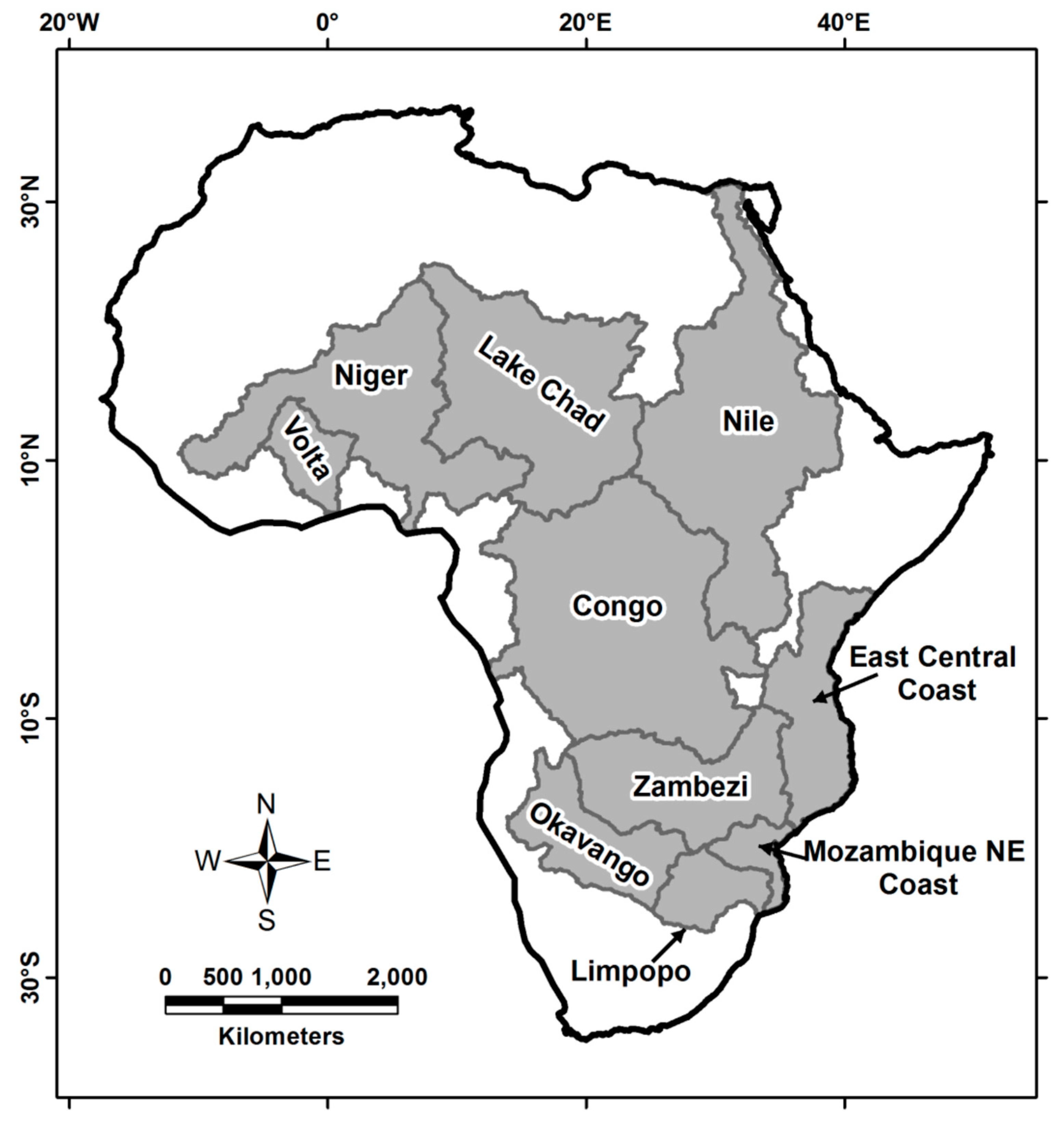
2. Materials and Methods

In the selection of model inputs process, we were guided by the water budget equation that explains the temporal variability in TWS_GRACE depending upon P, ET, and runoff. Given the fact that most of the African watersheds lack runoff data over the investigated period, T and NDVI data were used as model inputs instead. Both datasets are extracted from readily available datasets and expected to be correlated with TWS_GRACE. For example, an increase in soil moisture will increase NDVI and TWS, and an increase in temperature will increase evaporation and decrease TWS. Monthly NARX model input datasets, acquired over the time period of April 2002 to September 2015, were averaged over each of the examined African watersheds. A normalization technique was implemented to account for varying units, ranges, and magnitudes of the model input data. The normalization scales all input data in the range between 0 and 1 and ensures that all variables receive equal consideration. Normalization was applied using the following equation:

$${\widehat{x}}_t=\frac{x_t-x_{min}}{x_{max}-x_{min}}$$

(1)

where ${\widehat{x}}_t$ is the normalized value for a given input value $x_t$ at a given time t and $x_{max}$ and $x_{min}$ are the maximum and minimum recorded values of $x_t$, respectively.

2.1. Data

In this section, we briefly describe the inputs and target data used in the NARX model.

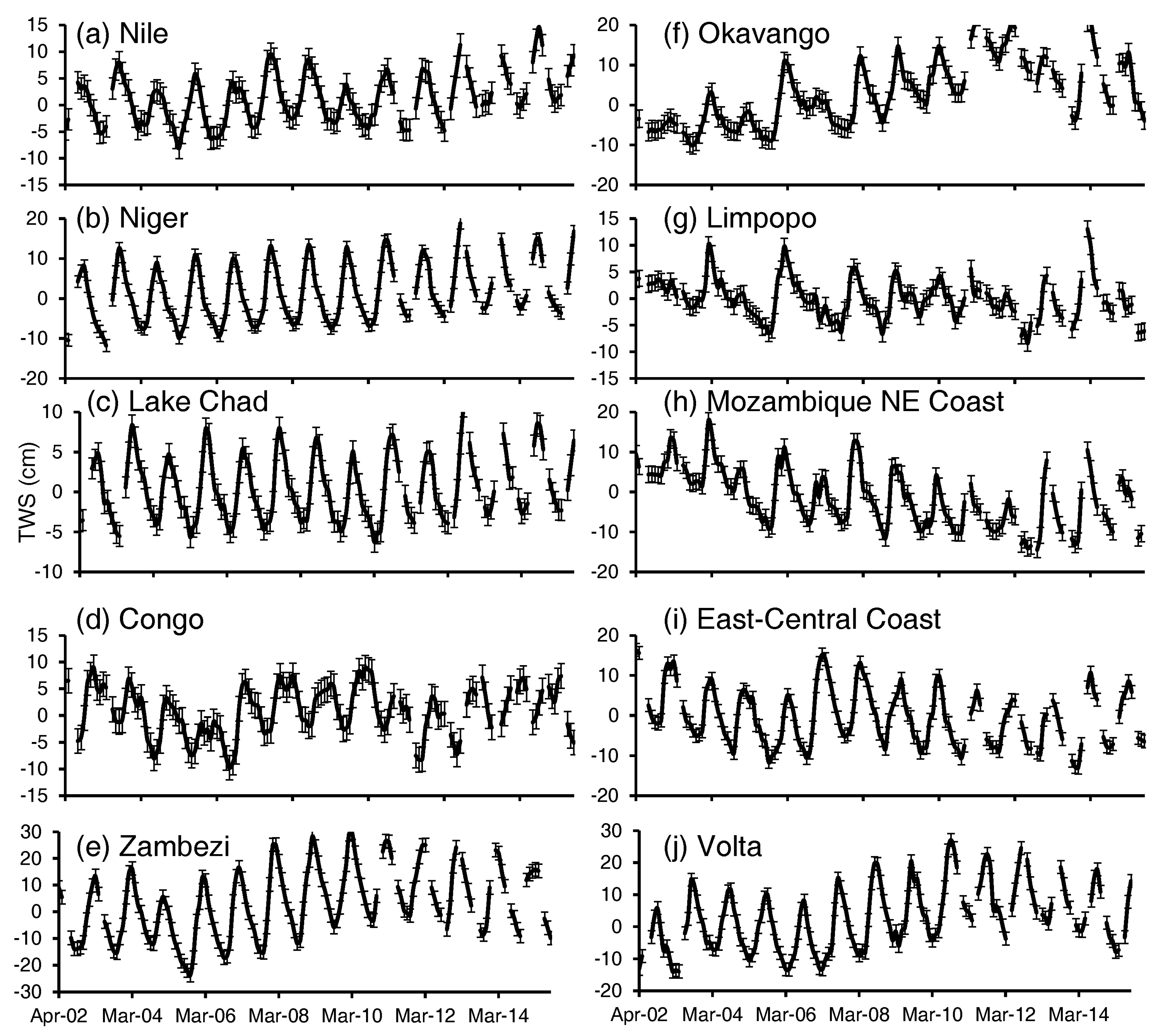
2.1.1. Gravity Recovery and Climate Experiment (GRACE)-derived Terrestrial Water Storage (TWS) (TWS_GRACE)

The most recent version (Release 06) of GRACE mascon solutions provided by the JPL (available at: https://podaac-opendap.jpl.nasa.gov/opendap/GeodeticsGravity/tellus/L3/mascon/) was used in this study. It has been reported that JPL mascon solutions provide a better reduction of leakage errors and improved signal localization [8]. Detailed description of processing steps used to generate JPL mascon solutions is provided in Watkins et al. [11] and Wiese at al. [81]. In summary, the Earth’s oblateness (C₂₀) and degree-1 (geocenter) coefficients provided by Cheng et al. [82] and Swenson et al. [83], respectively, were used. The glacial isostatic adjustment correction advanced by Peltier et al. [84] was applied. The temporal mean was removed. The Coastline Resolution Improvement (CRI) version, used in this study, were generated using the spherical caps (native resolution of GRACE mission, 3° the Equator, total: 4551 grids) approach and represented on 0.5° × 0.5° monthly TWS_GRACE girds. The basin averaged TWS_GRACE time series is calculated for each basin by averaging the results for all TWS_GRACE grid points lying within the spatial domain of each basin. These time series were then rescaled to restore true signal amplitude following the approach advanced by Landerer and Swenson [85]. Errors associated with basin averaged TWS_GRACE were quantified using the approach described in Ahmed and Abdelmohsen [18]. Figure 2 shows the temporal variations in TWS_GRACE averaged over each of the examined African watersheds.

2.1.2. Rainfall (P)

Rainfall data was extracted from the monthly Tropical Rainfall Measuring Mission (TRMM) dataset (available at: http://mirador.gsfc.nasa.gov/cgi-bin/mirador/presentNavigation.pl?project=TRMM&tree=project). TRMM provides near-global data with temporal and spatial sampling of 3 h and 0.25° × 0.25°, respectively [86]. TRMM-derived rainfall estimates provide adequate spatial and temporal correspondence with measured rainfall and stream flow data over most of the African watersheds [87,88,89,90].

2.1.3. Evapotranspiration (ET)

Evapotranspiration data was extracted from field-based ET measurements, the FLUXNET-Model Tree Ensembles (MTE) dataset. The FLUXNET-MTE (available at: https://www.bgc-jena.mpg.de/geodb/projects/Home.php) uses a machine learning algorithm to provide monthly global gridded (0.5° × 0.5°) estimates of sensible and latent heat fluxes from the eddy covariance towers network [91]. ET estimates were extracted from FLUXNET-MTE datasets given that the data is based on field measurements (i.e., flux tower measurements), and it has been successfully used by researchers to evaluate and/or calibrate remote sensing– and LSM-based ET estimates [3,92,93,94,95,96,97,98].

2.1.4. Temperature (T)

The air temperature data was extracted from the European Centre for Medium-Range Weather Forecasts (ECMWF) Re-Analysis (ERA Interim) project. The global ERA Interim (available at http://apps.ecmwf.int/datasets/data/interim-full-daily/levtype=sfc/) assimilates, using a 4-dimensional variational scheme, the 2 m air temperature using multiple sources of observational (e.g., station, satellite, and radiosonde) datasets at a temporal resolution of 6 hours and a spatial sampling of 0.75° × 0.75° [99]. The gridded ERA40 data shows similar short-term variability with Climate Research Unit (CRU) Temperature data version 2 (CRUTEM2v) derived directly from monthly station data [100]. Compared to ERA40 products, ERA Interim provides higher spatial and temporal resolutions as well as improved description of low-frequency variability and stratospheric circulation [101].

2.1.5. Normalized Difference Vegetation Index (NDVI)

The Moderate-resolution Imaging Spectroradiometer (MODIS)–derived NDVI products were used in this study. The NDVI data were generated from averaged level-3 MODIS Terra (MOD13C2) and MODIS Aqua (MYD13C2) products (available at https://lpdaac.usgs.gov/dataset_discovery/modis/modis_products_table). Both MOD13C2 and MYD13C2 are global monthly datasets with spatial sampling of 0.05° [102]. Significant correlations were reported between MODIS Terra and Aqua products over the majority of the African continent [103].

2.2. Approach

In this section, we describe the NARX model theory, structure, and performance measures.

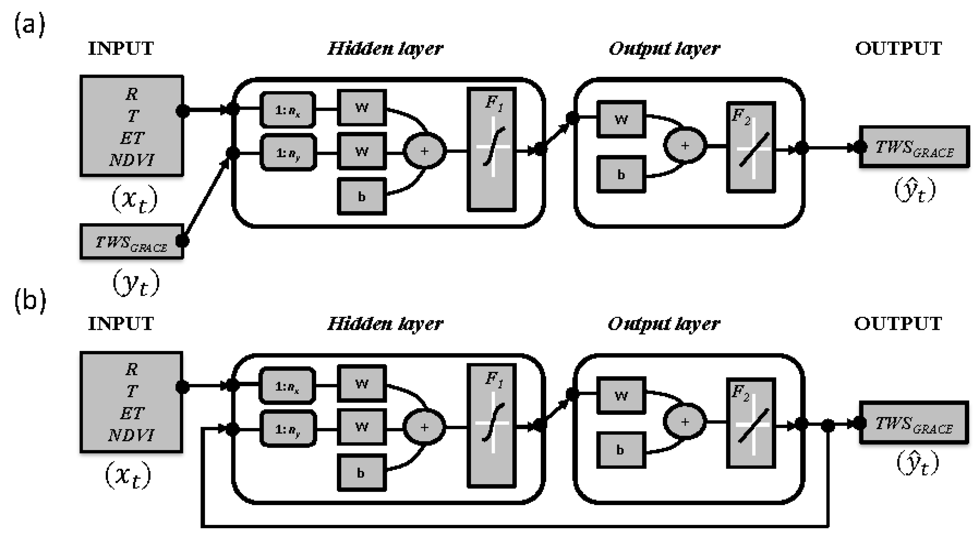
2.2.1. Nonlinear Autoregressive with Exogenous Input (NARX) Model

NARX model is used to derive relationships between TWS_GRACE data on the one hand and P, ET, T, and NDVI on the other hand. NARX is a recurrent dynamic ANN model with feedback connections enclosing several layers of the network [104,105]. NARX is designed to model nonlinear relations between the past inputs, past outputs, and the current output. In other words, the value of the output is regressed on previous values of the outputs and previous values of the inputs. The NARX model is formulated as a discrete time input–output recursive equations:

$${\widehat{y}}_{t+1}=f\left(y_t, y_{t-1},\dots , y_{t-n_y},x_{t+1}, x_t,x_{t-1},\dots , x_{t-n_x}\right)+{\epsilon }_{t+1},$$

(2a)

$${\widehat{y}}_{t+1}=f\left({\widehat{y}}_t, {\widehat{y}}_{t-1},\dots , {\widehat{y}}_{t-n_y},x_{t+1}, x_t,x_{t-1},\dots , x_{t-n_x}\right)+{\epsilon }_{t+1},$$

(2b)

where, ${\widehat{y}}_{t+1}$ is the NARX model output at the time $t+1$; ${\widehat{y}}_t, {\widehat{y}}_{t-1},\dots , {\widehat{y}}_{t-n_y}$ are the past outputs of the NARX model; $y_t, y_{t-1},\dots , y_{t-n_y}$ are the true past values of the time series (desired output values); $x_{t+1}, x_t,x_{t-1},\dots , x_{t-n_x}$ are the NARX model inputs; ${\epsilon }_t$ defines the error term, generally assumed to be Gaussian and white noise; $n_x$ and $n_y$ are the input and output orders of the dynamical model (e.g., delays), where $n_x\ge 0$ and $n_y\ge 1$; and $f$ is a nonlinear mapping function that is approximated by a regression model.

An alternative approach to NARX would have been to train several ANNs, each predicting TWS_GRACE with different lead times up to the maximum desired forecasting lead time. The two approaches are based on the same past measurements. The NARX approach forecasts targets after a recursive process and requires training only one model while the alternate approach predicts the targets directly but requires the calibration and validation of several models. It is unlikely that significant differences would have been observed using the multiple ANN approaches, the NARX approach was selected as it involves calibrating only one model.

The NARX model is expressed in two configurations, parallel architecture (also called closed-loop) and series-parallel (also called open-loop) architecture [106,107,108,109]. In the series-parallel architecture, which is useful for training, validation, and testing phases, the true output is used instead of feeding back the estimated output (Figure 3a). In other words, the future value of the time series ${\widehat{y}}_{t+1}$ is predicted from the present and past values of $x_t$ and true past values of the time series $y_t$. In the parallel architecture configuration, which is used in the prediction phase, the output is fed back to the input of the feedforward network (Figure 3b). In this case, the future value of the time series ${\widehat{y}}_{t+1}$ is predicted from the present and past values of $x_t$ and the past predicted values of the time series ${\widehat{y}}_t$. The open-loop configuration is expressed by Equation (2a), whereas, the closed-loop configuration is expressed by Equation (2b), e.g., [109].

In Equation (2), while the general functionality of the mapping function $\left(f\right)$ is known (usually a combination of sigmoid and linear type functions), the exact function is determined as part of the training phase of the NARX model. The NARX model is based on a Multi-Layer Perceptron (MLP) architecture consisting of three main layers: input, hidden, and output (target) layers. Hidden and output layers have associated activation functions for their respective neurons, each with weights and biases (Figure 3). Within the NARX model, the information flows, throughout the layers, from the input to the hidden layers, then to the output layers. In each layer, a scalar product ($x_j\times W_{ij})$ is calculated, by each neuron, by multiplying the input vector of the previous layer ($x_j)$by the weights vector ($W_{ij}$). The neurons outputs ($y_i$) are obtained by applying the activation function $F$ to the result of the scalar product:

$$y_i= F \left[{{\displaystyle \sum }}_{j=1}^n{x}_j. W_{ij}\right] ,$$

(3)

where, i and j are the neuron index in the layer and the input index in the NARX, respectively. Examples of activation functions $\left(F\right)$ include linear, sigmoid (logsig), and hyperbolic tangent (tansig). A tansig transfer function is utilized between the hidden layers as well as between input and hidden layers, whereas, a linear activation function is employed between hidden and output layers.

In the NARX training phase, the weights and biases of the ANN are progressively modified. The Bayesian regularization training function was selected to minimize a linear combination of squared errors and weights [106,109,110] while minimizing the chances of overfitting. The widely used Levenberg–Marquardt optimization method, e.g., [58] was selected to progressively update the ANN weights and biases. This approach was found to be fast and robust to train this study’s moderate-sized feedforward networks.

2.2.2. Nonlinear Autoregressive with Exogenous Input (NARX) Model Structure

In this study, four input variables (P, ET, T, and NDVI) are used to predict the target (TWS_GRACE) during the TWS_GRACE gap period and to forecast TWS_GRACE measurements 6 months ahead. To fill the TWS_GRACE gap, the NARX model used recent inputs up to the onset of the TWS_GRACE gap to predict the missing TWS_GRACE data. In the forecasting phase, we forecasted TWS_GRACE for “future” months where we do not have the benefit of concurrent or recent input data. To forecast TWS_GRACE data over African watersheds, we used “past” model inputs to predict the current or future TWS_GRACE data. The forecasting process was tested by increasing lead times from 1 up to 6 months in advance. For the one-month lead time, the model was used to predict the next TWS_GRACE data using previous inputs and TWS_GRACE data up to the time of prediction. The lead time was then increased while testing for different length of the input time series. The varying lead time approach was adopted based on our prior work [74] in which we reported varying lag times between the individual model inputs and the response in TWS_GRACE data.

NARX model was trained using 85% of the data and tested using the remaining 15%. Training and testing periods were selected randomly to maximize the model predictive capabilities by taking advantages of different wet and dry periods represented in the model input data. For consistency purposes, our results were displayed using April 2002–September 2013 and October 2013–September 2015 as training and testing periods, respectively. The NARX model was then used to forecast TWS_GRACE for the period from October 2015 through March 2016 (forecasting period).

Generally, the number of hidden neurons should range between half and twice the number of predictors [111,112]. In this study, the optimal number of hidden neurons was determined by trial and error, where the hidden neurons were added gradually until the predicted and measured values start to match while checking for potential model overfitting. The number of neurons in the hidden layer for the ten examined watersheds ranged from four to eight and a delay value ranging between 2 and 24 months was attempted. The delay value reflects, to some extent, the long-term dependence structures between the predicted target (e.g., TWS_GRACE) and the input variables (i.e., P, ET, T, and NDVI) [9,74].

Table 1. Nonlinear autoregressive with exogenous input (NARX) configurations along with simulations performance metrics.

Watershed	Architecture §	RMSE	R*	r	NSE	NSE*	Performance Category
Niger	4-8-1-13	1.91	0.30	0.95	0.91	0.62	Very Good
Volta	4-8-1-13	2.74	0.31	0.95	0.90	0.81	Very Good
Zambezi	4-8-1-7	2.56	0.24	0.97	0.94	0.81	Very Good
Okavango	4-8-1-13	2.72	0.37	0.95	0.86	0.72	Very Good
Lake Chad	4-8-1-13	1.40	0.39	0.93	0.84	0.55	Very Good
East Central Coast	4-8-1-13	3.09	0.44	0.91	0.80	0.45	Very Good
Mozambique NE Coast	4-8-1-7	3.47	0.52	0.93	0.71	0.31	Good
Congo	4-5-1-24	2.28	0.66	0.79	0.54	0.26	Satisfactory
Limpopo	4-4-1-10	3.16	0.63	0.91	0.59	0.20	Satisfactory
Nile	4-7-1-24	2.34	0.60	0.88	0.60	0.22	Satisfactory

^§ The four numbers represent the number of input layers, hidden neurons, output layers, and delay in each nonlinear autoregressive with exogenous input (NARX) network.

lists the architecture of the NARX network that generated the optimum results for each of the examined watersheds. The Monte Carlo simulations were used to measure the model stability, quantify the associated uncertainty, and improve the model generalization. We ran the NARX model for 50 runs, and the final TWS_GRACE predictions were calculated from the median of the model runs; the range of the model runs was used to estimate the uncertainties associated with the predicted TWS_GRACE. Automated regularization approach, advanced by MacKay [113], was used to optimize and overcome the overparameterization and generalization problems for each of these runs. In this approach, the parameters of the NARX model, with predetermined distributions, are assumed to be random. The regularization parameters, in this case, are attributed to the unknown variances associated with these distributions.

2.2.3. Performance Measures

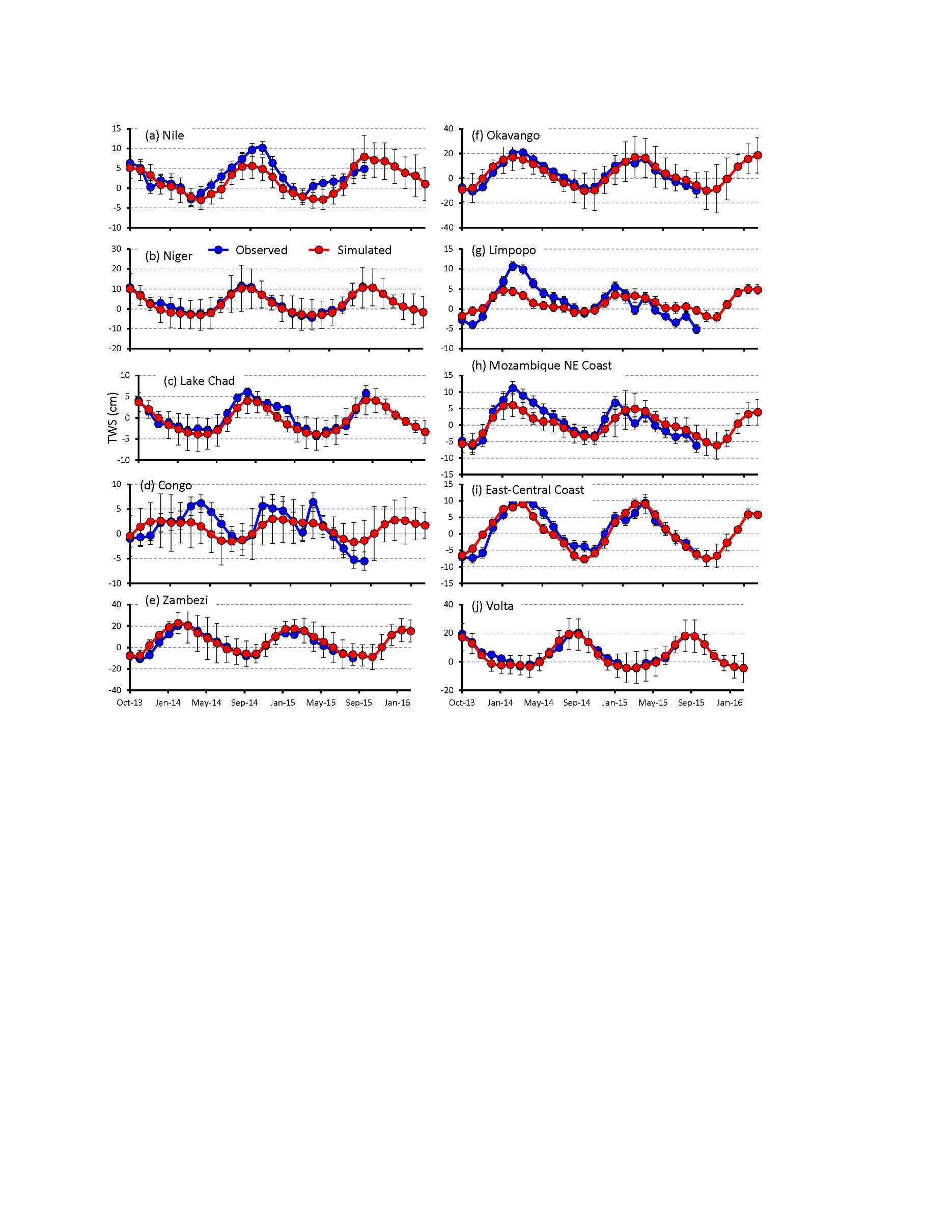
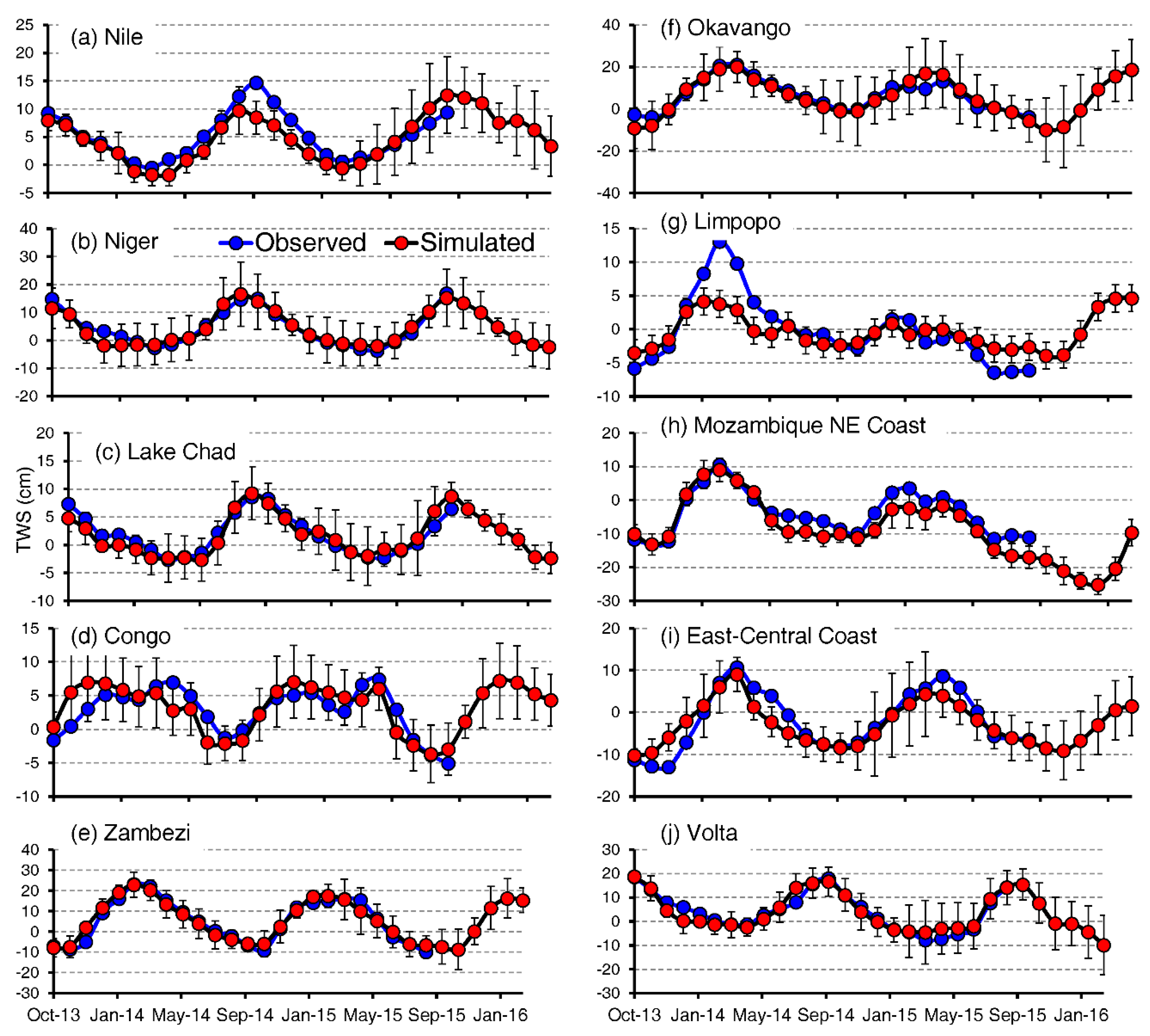
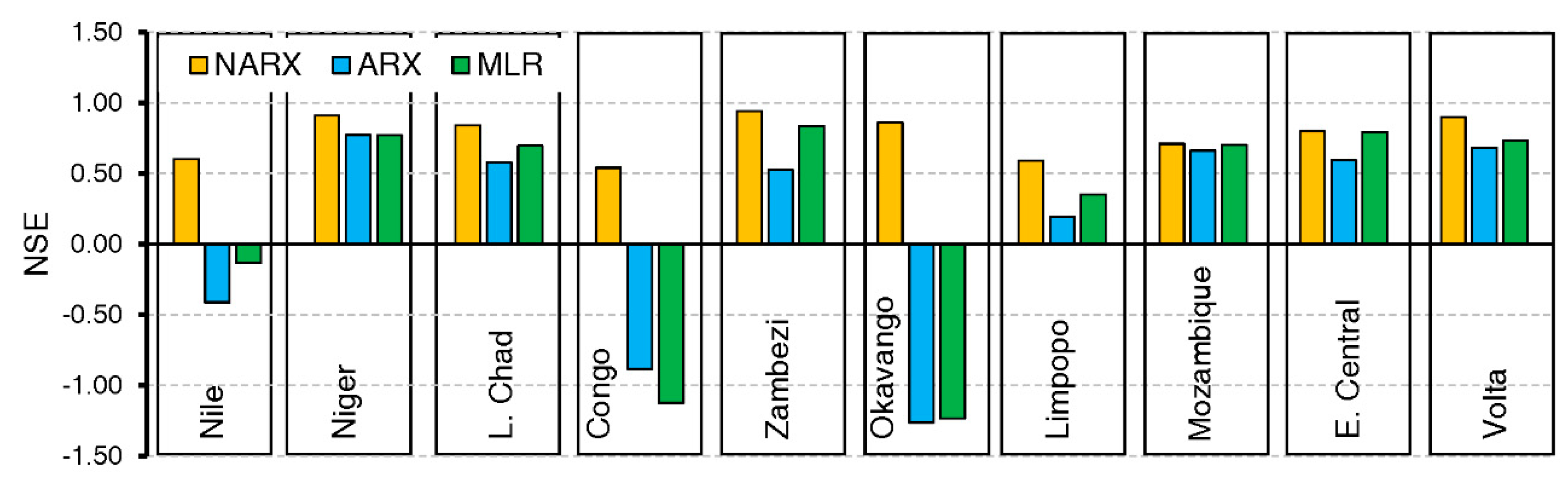
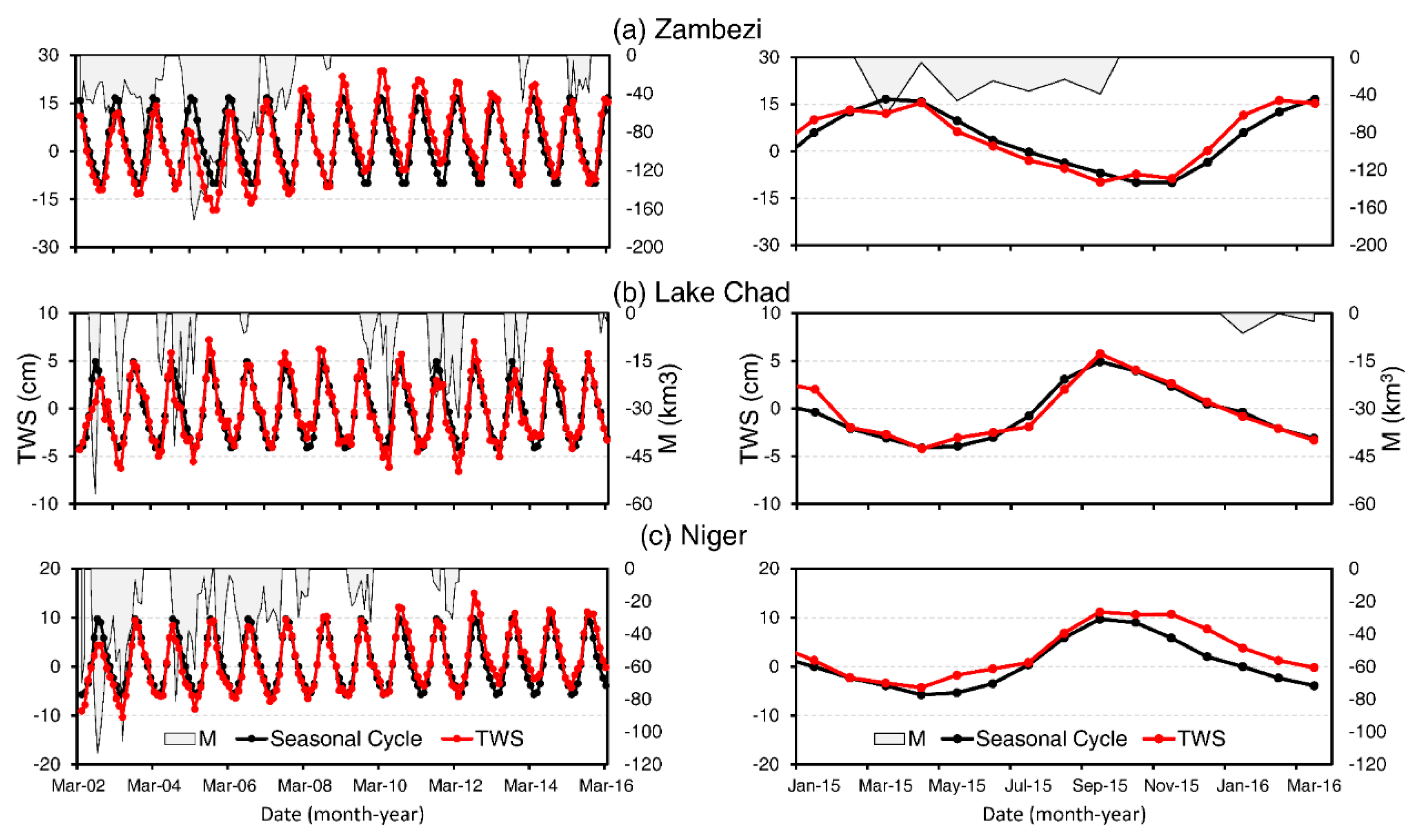
The performance of the NARX model was evaluated using several standard coefficients; Root mean square error (RMSE), scaled RMSE (R*), correlation coefficient (r), Nash–Sutcliffe efficiency (NSE) coefficient, and the seasonal adjusted NSE (NSE*) that are commonly used in the analysis and evaluation of statistical model results, in our case the NARX model outputs [114]. For example, NSE was found to be the best objective function for evaluating the overall fit between the predictive and observed values [115]. Likewise, r values were found to be sensitive to the differences between modeled and observed data including the extreme values (i.e., outliers) [116].

RMSE measures the global fitness of a predictive model by measuring the difference between the predicted and the observed values. Generally, lower RMSE indicate a better fit between the predicted and the observed values. RMSE is calculated as:

$$RMSE= \sqrt{\frac{{{\displaystyle \sum }}_{t=1}^n{(y_t-o_t)}^2}{n}}$$

(4)

where, $y_t$ and $o_t$ are the modelled and observed values at time (t), respectively, and n is the number of target data used for testing phase.

The scaled RMSE (R*) is defined as the ratio between RMSE and the standard deviation of observations ($\sigma )$ according to the following equation:

$$R^{*}= \frac{RMSE}{\sigma }$$

(5)

The correlation coefficient (r) is a measure of how likely future outcomes are to be predicted by the model. The value of r is obtained by dividing the covariance of the observed and modelled values by the product of their standard deviations according to the following equation:

$$r=\frac{{{\displaystyle \sum }}_{t=1}^n\left(y_t-\overline{y}\right)\left(o_t-\overline{o}\right)}{\sqrt{{{\displaystyle \sum }}_{t=1}^n{\left(y_t-\overline{y}\right)}^2}\sqrt{{{\displaystyle \sum }}_{t=1}^n{\left(o_t-\overline{o}\right)}^2}} ,$$

(6)

where the overbar denotes mean values. The value of r ranges between −1 and +1, where values of +1 and −1 indicate perfect increasing and decreasing linear relationships between variables, respectively, and a value of 0 indicates absence of such relationships between variables.

The NSE coefficient measures the predictive skill of a model relative to the mean of observations. In other words, NSE indicates how well the plot of observed versus modelled data fits the 1:1 line relationship [117]. The optimal value for the NSE is 1.0 and it is calculated using the following equation:

$$NSE=1- \frac{{{\displaystyle \sum }}_{t=1}^n{\left(y_t-o_t\right)}^2}{{{\displaystyle \sum }}_{t=1}^n{\left(o_t-\overline{o}\right)}^2},$$

(7)

The seasonal adjusted NSE coefficient (NSE*) takes into account the long-term annual cycle. NSE* was developed by Lorenz et al. [118] it is calculated using the following equation:

$$NS{E}^{*}=1- \frac{{{\displaystyle \sum }}_{t=1}^n{\left(y_t-o_t\right)}^2}{{{\displaystyle \sum }}_{t=1}^n{\left(o_t-\widehat{o}\right)}^2},$$

(8)

where $\widehat{o}$ is the long-term mean annual cycle. NSE* is greater than zero if the modelled time series is better than the long-term annual cycle and less than zero if the modelled time series cannot improve the long-term mean annual cycle with respect to the observations [118].

In this study, the model performance is classified into three main categories [73,114]: (a) very good performance if the resulting NSE is greater than 0.75 and R* is less than 0.50, (b) good performance if NSE is greater than 0.65 and R* is less than 0.60, and (c) satisfactory performance if NSE is greater than 0.5 and R* is less than 0.70.

3. Results

Table 1 shows the performance metrics of 50 runs of the NARX model over the investigated watersheds. The NARX model predictions (October 2013–September 2015) and forecasting (October 2015–March 2016) results over 10 African watersheds are shown in Figure 4. Examination of Table 1 shows that six watersheds (Niger, Volta, Zambezi, Okavango, Lake Chad, and East-Central Coast) show “very good” performance, one (Mozambique Northeast Coast) shows “good” performance, and the remaining three watersheds (Congo, Limpopo, and Nile) show “satisfactory” performance. The NSE* values are smaller than that of the NSE, but greater than zero, for all of the investigated African watersheds. Positive NSE* values indicate that the simulated TWS_GRACE time series agrees with the observed TWS_GRACE time series more than the values of the mean annual cycle. Thus, the NARX model is able to predict the seasonal and non-seasonal temporal variabilities.

Trial and error simulations, while avoiding overfitting, indicate that the performance of the NARX model is enhanced by increasing the training period and delays as well as number of input and hidden layers. For example, a delay of 13 months resulted in “very good” NARX model performance over the Niger, Volta, Okavango, Lake Chad, and East Central Coast basins. The performance of the NARX model, however, has not been improved with increasing the delay by more than 7 months in case of the Zambezi and the Mozambique Northeast Coast basins. The number of hidden layers was kept between half and twice the number of input layers. Eight hidden layers resulted in optimal NARX model performance over basins in the “very good” and “good” performance categories. Hidden layers exceeding eight in number resulted in model overfitting, reduced generalization, and increased training time. The Limpopo, Congo, and Nile basins were assigned 4, 5, and 7 hidden layers, respectively. Fewer hidden layers (<4) resulted in NARX model underfitting.

NARX model results over the African watersheds were compared to results from other ANN models (nonlinear autoregressive exogenous [ARX]) as well as results from multilinear regression (MLR) model. Unlike the NARX model, the ARX model identifies nonlinear relations between the past inputs and the current output using the following equation:

$${\widehat{y}}_t=f\left(x_{t-1},x_{t-2},\dots ,x_{t-n_x}\right)+{\epsilon }_t,$$

(9)

The same architecture listed in Table 1 was used for the ARX model.

The MLR model, on the other hand, maps the linear relationships between the current inputs and the current output according to the following equation:

$${\widehat{y}}_t=a_0+a_1{x}_{1t}+a_2{x}_{2t}+\cdots +a_n{x}_{nt}+{\epsilon }_t ,$$

(10)

where $a_0$ is the intercept and $a_1, \dots , a_n$ are the model coefficients.

Figure 5 shows the NSE values for NARX, ARX, and MLR models over the investigated African watersheds. Examination of Figure 5 indicates that the NSE values of the ARX and MLR models are always lower than that of the NARX model. For the Nile, Congo, and Okavango basins, the NSE of the ARX and MLR models are negative, indicating that the simulated TWS_GRACE means are worse than the observed TWS_GRACE means. One reason for the better performance of the NRAX compared to the other models could be the nature of the spatiotemporal variabilities of TWS_GRACE over the African watersheds and how they are related to episodic changes in natural variability (e.g., rainfall, temperature, etc.), as well as long-term natural and anthropogenic changes in storage (e.g., soil moisture, groundwater) signals.

The forecasted TWS_GRACE could potentially be used in several hydrological applications. We provide one demonstration for a potential application, where the projected TWS_GRACE was used to forecast the hydrological drought events in three African watersheds (Zambezi, Lake Chad, and Niger basins). Thomas et al. [119] used the TWS_GRACE to quantify the monthly water storage deficits. The latter provides a direct measure of the magnitude of the volumetric departure from “normal” hydrological conditions. We applied the same approach to forecast the hydrological drought using the NARX-derived TWS_GRACE. We first calculated the mean monthly seasonal cycle by averaging each of the 12 months (January, February, etc.) in the TWS_GRACE time series. The seasonal cycle was then subtracted from the observed TWS_GRACE time series. Negative difference indicated TWS_GRACE deficits defined as (M). M (in km³) represents the volume of water required, in any month, to return to normal conditions and is calculated by multiplying the negative difference by the basin area. A hydrological drought event is identified if M lasts three or more continuous months [119]. Figure 6 shows the GRACE-derived hydrological drought events over Zambezi (Figure 6a), Lake Chad (Figure 6b), and Niger basins (Figure 6c). Examination of Figure 6 shows that during the forecasted TWS_GRACE period (October 2015–March 2016), no drought events were observed over the Niger basin, the latest (March–October 2015) drought event over the Zambezi basin came to an end, and the Lake Chad basin witnessed the onset of a drought event (January–March 2016). Analysis of different datasets (e.g., rainfall, temperature, climate indices) confirmed the 2016 drought in the Zambezi basin [120].

4. Discussion

The relatively lower performance of the NARX model over the Congo, Limpopo, and Nile basins could be attributed to poor correspondence of TWS_GRACE with the 6 months lead time of one or more of the input variables (P, ET, T, and NDVI) or the absence of one or more of the important controlling and/or related factors. Other factors that could affect the NARX model performance include the climatic settings, climate cyclicity, and anthropogenic factors. It is worth mentioning that the performance of a NARX model is generally enhanced by the presence of more “dynamics” in the training phase [121]. For example, the Limpopo basin lacks the strong seasonal patterns that were observed over the other investigated basins (Figure 2g). In addition, the Limpopo basin exhibits the lowest TWS_GRACE amplitude of annual cycle (6.09 cm) compared to other investigated watersheds (range: 9.20 cm to 30.44 cm). The Limpopo basin also experiences anthropogenic activities. During the investigated period, the Limpopo basin experienced the constructions of the Ntimbale (year: 2009; capacity: 0.26 km³), Dikgatlhong (year: 2012; capacity: 4.0 km³), Thune (year: 2012; capacity: 0.90 km³), and Lotsane (year: 2012; capacity: 0.40 km³) dams in Botswana and the Massingir dam (year: 2008; capacity: 2.8 km³) in Mozambique. The anthropogenic activities change the portioning of TWS_GRACE components as well as the phase, amplitude, residual signals, and trend of TWS_GRACE time series [9]. The dynamics/seasonality in the Nile basin is clear (Figure 2a), yet the basin extends over several climatic settings (tropical, semi-arid, arid, and Mediterranean), experiences anthropogenic activities (e.g., construction of Merowe, Tekeze, Amerti-Neshi, and Millennium dams, heightened of Roseiris, Jebel Aulia, Khashm El Gibta dams, and groundwater extraction in the Western Desert of Egypt; [9]). The Nile Basin also witnesses climatic cyclicity (64-, 19-, 12-, and 7-year cycles) [122]. The 7-year cycle could be well represented in the training period, but the 64-, 19-, and 12-year cycles are not, given the short time span of the training period (12-year).

Likewise, the Congo basin is also experiencing anthropogenic activities (i.e., deforestation activities; [9]) and is apparently witnessing multi-year and decadal climatic cycles. Ahmed et al. [9] reported a decrease in annual NDVI that was consistent with the increase in the annual deforestation rates. Annual deforestation rates for the Ubangi, Sangha, and Congo subbasins of the Congo basin are on the rise (period 1990–2000: 0.58%, 0.38%, and 0.20%; 2000–2005: 0.62%, 0.40%, and 0.21%; 2005–2010: 0.65%, 0.41%, and 0.22%). In addition, the rainfall patterns over the Congo basin are cyclic in nature. They range from multi-year (cycles: 2–8 year) oscillations [123,124], to near-decadal, decadal, and multi-decadal fluctuations [123,125,126]. These cyclicity patterns in precipitation are reflected in the fluctuations in basin discharge (fluctuations in basin discharge: 2–4, 6–8, 13–15, and 30–35 year; [127,128,129]). Multi-year cycles are apparently observed in the TWS_GRACE trend data (Figure 2d). Piecewise trend analysis of TWS_GRACE averaged over the Congo basin (Figure 2d) showed significant TWS_GRACE depletion (−22.9 mm/yr) from 2002 to 2006, near-steady state conditions (−1.35 mm/yr) from 2006 to 2011, and signs of significant increase in TWS_GRACE (+10.7 mm/yr) from 2011 to 2015. Again, given the short time span covered by the GRACE mission, the incorporation of the prolonged cycles in the NARX model over the Congo basin was not enabled.

The launch of the GRACE-FO mission and the acquisition of TWS_GRACE data over the upcoming years, together with those acquired throughout the GRACE mission, will enable the construction of a continuous decadal TWS record. The latter will undoubtedly enhance model performance over basins that experience decadal climatic cyclicities such as the Congo and Nile basins given the prolonged time periods that are needed for the NARX model to learn over such basins.

5. Conclusions

The currently available TWS_GRACE time series suffers from gaps in temporal records due to battery performance issues. In addition, a minimum of one-year TWS data gap exists between the past GRACE and current GRACE-FO missions. We developed and implemented a statistical approach that predicts and forecasts TWS_GRACE time series 6 months in advance and tested the developed approach over 10 major African watersheds. The NARX model was used to derive relationships between TWS_GRACE data (target) and the controlling and/or related factors (P, T, ET, and NDVI) over the selected watersheds. The performance of the developed model was evaluated using several coefficients and was found to be “very good” over six watersheds (Niger, Volta, Zambezi, Okavango, Lake Chad, and East-Central Coast), “good” over one (Mozambique Northeast Coast) and “satisfactory” over the remaining three watersheds (Congo, Limpopo, and Nile). The “satisfactory” performance over these three basins is attributed here to one or more of the following: (1) the watershed witnessing anthropogenic activities, (2) the watershed extending over multiple climatic settings, and (3) prolonged (e.g., decadal) climatic cyclicity that is not adequately represented in the model training period. In addition, the modeled TWS_GRACE were used to forecast the severity of droughts over the Zambezi, Lake Chad, and Niger basins. During the forecasted TWS_GRACE period, no drought events were observed over the Niger basin, the latest (March–October 2015) drought event over the Zambezi basin came to an end, and the Lake Chad basin witnessed the onset of a drought event (January–March 2016). Although not demonstrated here, the forecasted TWS could potentially be used to address a wide range of hydrological applications, including forecasting seasonal and inter-annual spatiotemporal variations in TWS over river basins, basin-scale ET, and natural/climatic and anthropogenic impacts on continental aquifer systems, and flood events.

Our approach is robust, effective, and advantageous, given the following: (1) the model does not require knowledge of basin characteristics and could be applied to relatively small basins (as small as 63,000 km²) that could be resolved by GRACE data [130]; (2) our approach forecasts TWS_GRACE time series 6 months in advance; (3) the significant forecasting time period for TWS_GRACE of our model could be used to project TWS_GRACE within various watersheds and thus could potentially be used for developing sound, year-to-year, sustainable water management scenarios for these watersheds; (4) our approach considers the full spatiotemporal and spectral signatures of TWS_GRACE time series (e.g., seasonal and sub seasonal, trend, and residual terms); (5) our model provides high TWS_GRACE predictability values; and (6) the model could potentially be modified to enable applications over a wide range of drainage basins and settings by incorporating additional variables (e.g., snow-related variables) and could potentially enable long term predictions once longer training time periods could be attained.

Our NARX model was successfully tested over a wide range of climatic and hydrologic settings across the entire continent of Africa including tropical and subtropical systems. Thus, it could potentially be applied to large sectors of the globe with similar climatic zones and hydrologic settings in South and Central America, Australia, and southern Asia. These areas cover approximately 60% of the Earth’s continental surface. Our NARX model will have to be modified if we were to apply it to the remaining continental masses including polar, boreal, and temperate areas where the water budget of the hydrologic systems is partially or largely controlled by, or correlated with, snow parameters (e.g., snow fall, snow melt). In such areas, one would expect that snow-related parameters would have to be incorporated in the modified NARX model to adequately account for the observed TWS_GRACE over these areas. In other words, multiple NARX models will have to be constructed if we were to apply this approach on a global scale. Studies should concentrate on evaluating the extent to which the advanced and advocated procedures could be applied to predict and forecast pixel-based TWS_GRACE datasets, as opposed to watershed-based predictions. Although not shown, our preliminary results are encouraging and if successful, this will benefit the GRACE user community at large. The NARX model could be generally used as Kalman prediction and data update or prediction only in case of no TWS_GRACE data.

The applications of techniques such as those applied and advocated here and the acquisition of TWS_GRACE data over the upcoming years by GRACE-FO and GRACE-II (planned in 2025) missions could potentially enable the construction of continuous uninterrupted decadal TWS_GRACE records over the major hydrologic systems across the globe. These records could be readily used to enhance the current TWS_GRACE hydrologic applications and provide predictive tools that could address a wide range of environmental and hydrological problems.

The developed approach is of timely importance as well given the degradation of GRACE operational capability specifically during the last couple months of the mission lifetime, as manifested by the increase in the number of data gaps with time due to battery performance issues. For example, the data gaps increased from 3 months for the period April 2002 to December 2010 to 17 months for the period January 2011 to June 2017. In October 2017, NASA decommissioned the GRACE-2 satellite and ended the GRACE science mission. This decision was based on an age-related battery issue; the remaining battery capacity could no longer operate the science instruments and telemetry transmitter on board GRACE-2. There is an urgent need to develop approaches to construct a continuous and an uninterrupted TWS_GRACE record that encompasses GRACE and GRACE–FO mission datasets and fills the gap between these two missions. The applied and the advocated methodologies could assist in achieving this goal.

References

1. Tapley, B.D.; Bettadpur, S.; Ries, J.C.; Thompson, P.F.; Watkins, M.M. GRACE measurements of mass variability in the Earth system. Science 2004, 305, 503–505. [Google Scholar] [CrossRef] [PubMed]
2. Wahr, J.; Molenaar, M.; Bryan, F. Time variability of the Earth’s gravity field: Hydrological and oceanic effects and their possible detection using GRACE. J. Geophys. Res. 1998, 103, 30205–30229. [Google Scholar] [CrossRef]
3. Ahmed, M.; Sultan, M.; Yan, E.; Wahr, J. Assessing and Improving Land Surface Model Outputs over Africa using GRACE, Field, and Remote Sensing Data. Surv. Geophys. 2016, 37, 529–556. [Google Scholar] [CrossRef]
4. Mohamed, A.; Sultan, M.; Ahmed, M.; Yan, E.; Ahmed, E. Aquifer recharge, depletion, and connectivity: Inferences from GRACE, land surface models, geochemical, and geophysical data. GSA Bull. 2016, 129, 1–13. [Google Scholar] [CrossRef]
5. Famiglietti, J.S. The global groundwater crisis. Nat. Clim. Chang. 2014, 4, 945–948. [Google Scholar] [CrossRef]
6. Jacob, T.; Wahr, J.; Pfeffer, W.T.; Swenson, S. Recent contributions of glaciers and ice caps to sea level rise. Nature 2012, 482, 514–518. [Google Scholar] [CrossRef] [PubMed]
7. Tapley, B.; Watkins, M.M.; Flechtner, F.; Reigber, C.; Bettadpur, S.; Rodell, M.; Famiglietti, J.; Landerer, F.; Chambers, D.; Reager, J.; et al. Contributions of GRACE to understanding climate change. Nat. Clim. Chang. 2019, 9, 358–369. [Google Scholar] [CrossRef]
8. Rodell, M.; Famiglietti, J.S.; Wiese, D.N.; Reager, J.T.; Beaudoing, H.K.; Landerer, F.W.; Lo, M.H. Emerging trends in global freshwater availability. Nature 2018, 557, 651–659. [Google Scholar] [CrossRef]
9. Ahmed, M.; Sultan, M.; Wahr, J.; Yan, E. The use of GRACE data to monitor natural and anthropogenic induced variations in water availability across Africa. Earth-Sci. Rev. 2014, 136, 289–300. [Google Scholar] [CrossRef]
10. Save, H.; Bettadpur, S.; Tapley, B. High resolution CSR GRACE RL05 mascons. J. Geophys. Res. 2016, 121, 7547–7569. [Google Scholar] [CrossRef]
11. Watkins, M.M.; Wiese, D.N.; Yuan, D.; Boening, C.; Landerer, F.W. Improved methods for observing Earth’s time variable mass distribution with GRACE using spherical cap mascons. J. Geophys. Res. Solid Earth 2015, 120, 2648–2671. [Google Scholar] [CrossRef]
12. Voss, K.A.; Famiglietti, J.S.; Lo, M.; De Linage, C.; Rodell, M.; Swenson, S.C. Groundwater depletion in the Middle East from GRACE with implications for transboundary water management in the Tigris-Euphrates-Western Iran region. Water Resour. Res. 2013, 49, 904–914. [Google Scholar] [CrossRef] [PubMed] [Green Version]
13. Feng, W.; Zhong, M.; Lemoine, J.-M.; Biancale, R.; Hsu, H.-T.; Xia, J. Evaluation of groundwater depletion in North China using the Gravity Recovery and Climate Experiment (GRACE) data and ground-based measurements. Water Resour. Res. 2013, 49, 2110–2118. [Google Scholar] [CrossRef]
14. Joodaki, G.; Wahr, J.; Swenson, S. Estimating the human contribution to groundwater depletion in theMiddle East, fromGRACE data, land surfacemodels, and well observations. Water Resour. Res. 2014, 50, 1–14. [Google Scholar] [CrossRef]
15. Castle, S.; Thomas, B.; Reager, J.; Rodell, M.; Swenson, S.; Famiglietti, J. Groundwater depleation during drought threatens future water security of the Colorado River Basin. Geophys. Res. Lett. 2014, 10, 5904–5911. [Google Scholar] [CrossRef] [PubMed]
16. Fallatah, O.A.; Ahmed, M.; Save, H.; Akanda, A.S. Quantifying Temporal Variations in Water Resources of a Vulnerable Middle Eastern Transboundary Aquifer System. Hydrol. Process. 2017, 31, 4081–4091. [Google Scholar] [CrossRef]
17. Fallatah, O.A.; Ahmed, M.; Cardace, D.; Boving, T.; Akanda, A.S. Assessment of Modern Recharge to Arid Region Aquifers Using an Integrated Geophysical, Geochemical, and Remote Sensing Approach. J. Hydrol. 2018. [Google Scholar] [CrossRef]
18. Ahmed, M.; Abdelmohsen, K. Quantifying Modern Recharge and Depletion Rates of the Nubian Aquifer in Egypt. Surv. Geophys. 2018, 39, 729–751. [Google Scholar] [CrossRef]
19. Houborg, R.; Rodell, M.; Li, B.; Reichle, R.; Zaitchik, B.F. Drought indicators based on model-assimilated Gravity Recovery and Climate Experiment (GRACE) terrestrial water storage observations. Water Resour. Res. 2012, 48. [Google Scholar] [CrossRef] [Green Version]
20. Eicker, A.; Schumacher, M.; Kusche, J.; Döll, P.; Schmied, H.M. Calibration/Data Assimilation Approach for Integrating GRACE Data into the WaterGAP Global Hydrology Model (WGHM) Using an Ensemble Kalman Filter: First Results. Surv. Geophys. 2014, 35, 1285–1309. [Google Scholar] [CrossRef]
21. Zaitchik, B.F.; Rodell, M.; Reichle, R.H. Assimilation of GRACE Terrestrial Water Storage Data into a Land Surface Model: Results for the Mississippi River Basin. J. Hydrometeorol. 2008, 9, 535–548. [Google Scholar] [CrossRef]
22. Gruber, C.; Gouweleeuw, B. Short-latency monitoring of continental, ocean- and atmospheric mass variations using GRACE intersatellite accelerations. Geophys. J. Int. 2019, 217, 714–728. [Google Scholar] [CrossRef] [Green Version]
23. Famiglietti, J.S.; Rodell, M. Water in the balance. Science 2013, 340, 1300–1301. [Google Scholar] [CrossRef] [PubMed]
24. Reager, J.T.; Famiglietti, J.S. Characteristic mega-basin water storage behavior using GRACE. Water Resour. Res. 2013, 49, 3314–3329. [Google Scholar] [CrossRef] [PubMed] [Green Version]
25. Döll, P.; Müller Schmied, H.; Schuh, C.; Portmann, F.T.; Eicker, A. Global-scale assessment of groundwater depletion and related groundwater abstractions: Combining hydrological modeling with information from well observations and GRACE satellites. Water Resour. Res. 2014, 50, 5698–5720. [Google Scholar] [CrossRef]
26. Güntner, A.; Stuck, J.; Werth, S.; Döll, P.; Verzano, K.; Merz, B. A global analysis of temporal and spatial variations in continental water storage. Water Resour. Res. 2007, 43, 1–19. [Google Scholar] [CrossRef]
27. Humphrey, V.; Gudmundsson, L.; Seneviratne, S.I. Assessing Global Water Storage Variability from GRACE: Trends, Seasonal Cycle, Subseasonal Anomalies and Extremes. Surv. Geophys. 2016, 37, 357–395. [Google Scholar] [CrossRef] [Green Version]
28. Döll, P.; Fritsche, M.; Eicker, A.; Müller Schmied, H. Seasonal Water Storage Variations as Impacted by Water Abstractions: Comparing the Output of a Global Hydrological Model with GRACE and GPS Observations. Surv. Geophys. 2014, 35, 1311–1331. [Google Scholar] [CrossRef]
29. Forootan, E.; Safari, A.; Mostafaie, A.; Schumacher, M.; Delavar, M.; Awange, J.L. Large-Scale Total Water Storage and Water Flux Changes over the Arid and Semiarid Parts of the Middle East from GRACE and Reanalysis Products. Surv. Geophys. 2016, 1–25. [Google Scholar] [CrossRef]
30. Harvey, C.L.; Dixon, H.; Hannaford, J. Developing best practice for infilling daily river flow data. Br. Hydrol. Soc. 2010, 816–823. [Google Scholar] [CrossRef]
31. Soro, G.; Noufé, D.; Goula Bi, T.; Shorohou, B. Trend Analysis for Extreme Rainfall at Sub-Daily and Daily Timescales in Côte d’Ivoire. Climate 2016, 4, 37. [Google Scholar] [CrossRef]
32. Machiwal, D.; Kumar, S.; Dayal, D. Characterizing rainfall of hot arid region by using time-series modeling and sustainability approaches: A case study from Gujarat, India. Theor. Appl. Climatol. 2016, 124, 593–607. [Google Scholar] [CrossRef]
33. Adeloye, A.J.; Montaseri, M. Preliminary streamflow data analyses prior to water resources planning study. Hydrol. Sci. J. 2002, 47, 679–692. [Google Scholar] [CrossRef]
34. Adamowski, K.; Bougadis, J. Detection of trends in annual extreme rainfall. Hydrol. Process. 2003, 17, 3547–3560. [Google Scholar] [CrossRef]
35. Markonis, Y.; Koutsoyiannis, D. Climatic Variability over Time Scales Spanning Nine Orders of Magnitude: Connecting Milankovitch Cycles with Hurst–Kolmogorov Dynamics. Surv. Geophys. 2013, 34, 181–207. [Google Scholar] [CrossRef]
36. Jin, S.; Zhang, T. Terrestrial Water Storage Anomalies Associated with Drought in Southwestern USA from GPS Observations. Surv. Geophys. 2016, 37, 1139–1156. [Google Scholar] [CrossRef]
37. Yozgatligil, C.; Aslan, S.; Iyigun, C.; Batmaz, I. Comparison of missing value imputation methods in time series: The case of Turkish meteorological data. Theor. Appl. Climatol. 2013, 112, 143–167. [Google Scholar] [CrossRef]
38. Campozano, L.; Sánchez, E.; Aviles, A.; Samaniego, E. Evaluation of infilling methods for time series of daily precipitation and temperature: The case of the Ecuadorian Andes. Maskana 2014, 5, 99–115. [Google Scholar] [CrossRef]
39. Beauchamp, J.J.; Downing, D.J.; Railsback, S.F. Comparison of regression and time-series methods for synthesizing missing streamflow records. J. Am. Water Resour. Assoc. 1989, 25, 961–975. [Google Scholar] [CrossRef]
40. Gould, P.G.; Koehler, A.B.; Ord, J.K.; Snyder, R.D.; Hyndman, R.J.; Vahid-Araghi, F. Forecasting time series with multiple seasonal patterns. Eur. J. Oper. Res. 2008, 191, 207–222. [Google Scholar] [CrossRef]
41. Mwale, F.D.; Adeloye, A.J.; Rustum, R. Infilling of missing rainfall and streamflow data in the Shire River basin, Malawi—A self organizing map approach. Phys. Chem. Earth Parts A/B/C 2012, 50, 34–43. [Google Scholar] [CrossRef]
42. Infilling missing daily precipitation data at multiple sites using a multivariate truncated normal distribution model. Available online: http://adsabs.harvard.edu/abs/2009AGUFM.H31D0813N (accessed on 27 July 2019).
43. Tum, M.; Günther, K.P.; Böttcher, M.; Baret, F.; Bittner, M.; Brockmann, C.; Weiss, M. Global gap-free MERIS LAI time series (2002–2012). Remote Sens. 2016, 8, 69. [Google Scholar] [CrossRef]
44. Hasan, E. The challenges and opportunities of hydrologic remote sensing in data-poor regions: Case study of Nile River Basin. In Proceedings of the AGU Fall Meeting 2015, San Francisco, CA, USA, 14–18 December 2015. [Google Scholar]
45. Long, D.; Scanlon, B.R.; Longuevergne, L.; Sun, A.Y.; Fernando, D.N.; Save, H. GRACE satellite monitoring of large depletion in water storage in response to the 2011 drought in Texas. Geophys. Res. Lett. 2013, 40, 3395–3401. [Google Scholar] [CrossRef] [Green Version]
46. Rodell, M.; Houser, P.R.; Jambor, U.; Gottschalck, J.; Mitchell, K.; Meng, C.-J.; Arsenault, K.; Cosgrove, B.; Radakovich, J.; Bosilovich, M.; et al. The global land data assimilation system. Bull. Am. Meteorol. Soc. 2004, 85, 381–394. [Google Scholar] [CrossRef]
47. Oleson, K.W.; Niu, G.Y.; Yang, Z.L.; Lawrence, D.M.; Thornton, P.E.; Lawrence, P.J.; Stöckli, R.; Dickinson, R.E.; Bonan, G.B.; Levis, S.; et al. Improvements to the community land model and their impact on the hydrological cycle. J. Geophys. Res. Biogeosci. 2008, 113. [Google Scholar] [CrossRef]
48. Döll, P.; Kaspar, F.; Lehner, B. A global hydrological model for deriving water availability indicators: Model tuning and validation. J. Hydrol. 2003, 270, 105–134. [Google Scholar] [CrossRef]
49. Fan, Y.; van den Dool, H. Climate Prediction Center global monthly soil moisture data set at 0.5° resolution for 1948 to present. J. Geophys. Res. Atmos. 2004, 109, 1–8. [Google Scholar] [CrossRef]
50. Forootan, E.; Kusche, J.; Loth, I.; Schuh, W.-D.; Eicker, A.; Awange, J.; Longuevergne, L.; Diekkrüger, B.; Schmidt, M.; Shum, C.K. Multivariate Prediction of Total Water Storage Changes over West Africa from Multi-Satellite Data. Surv. Geophys. 2014, 35, 913–940. [Google Scholar] [CrossRef]
51. De Linage, C.; Famiglietti, J.S.; Randerson, J.T. Statistical prediction of terrestrial water storage changes in the Amazon Basin using tropical Pacific and North Atlantic sea surface temperature anomalies. Hydrol. Earth Syst. Sci. 2014, 18, 2089–2102. [Google Scholar] [CrossRef] [Green Version]
52. Rietbroek, R.; Fritsche, M.; Dahle, C.; Brunnabend, S.-E.; Behnisch, M.; Kusche, J.; Flechtner, F.; Schröter, J.; Dietrich, R. Can GPS-Derived Surface Loading Bridge a GRACE Mission Gap? Surv. Geophys. 2014, 35, 1267–1283. [Google Scholar] [CrossRef] [Green Version]
53. Wahr, J.; Burgess, E.; Swenson, S. Using GRACE and climate model simulations to predict mass loss of Alaskan glaciers through 2100. J. Glaciol. 2016, 62, 623–639. [Google Scholar] [CrossRef] [Green Version]
54. Becker, M.; Meyssignac, B.; Xavier, L.; Cazenave, A.; Alkama, R.; Decharme, B. Past terrestrial water storage (1980–2008) in the Amazon Basin reconstructed from GRACE and in situ river gauging data. Hydrol. Earth Syst. Sci. 2011, 15, 533–546. [Google Scholar] [CrossRef]
55. Humphrey, V.; Gudmundsson, L.; Seneviratne, S.I. A global reconstruction of climate-driven subdecadal water storage variability. Geophys. Res. Lett. 2017, 44, 2300–2309. [Google Scholar] [CrossRef]
56. Long, D.; Shen, Y.; Sun, A.; Hong, Y.; Longuevergne, L.; Yang, Y.; Li, B.; Chen, L. Remote Sensing of Environment Drought and fl ood monitoring for a large karst plateau in Southwest China using extended GRACE data. Remote Sens. Environ. 2014, 155, 145–160. [Google Scholar] [CrossRef]
57. Ferreira, V.; Andam-Akorful, S.; Dannouf, R.; Adu-Afari, E. A Multi-Sourced Data Retrodiction of Remotely Sensed Terrestrial Water Storage Changes for West Africa. Water 2019, 11, 401. [Google Scholar] [CrossRef]
58. Haykin, S. Neural Networks: A Comprehensive Foundation; Prentice-Hall, Inc.: Upper Saddle River, NJ, USA, 1999. [Google Scholar]
59. Gurney, K. An Introduction to Neural Networks; UCL Press Limited: London, UK, 1997; ISBN 0203451511. [Google Scholar]
60. Govindaraju, R.S.; Rao, A.R.; Adiseshappa, R. Artificial Neural Networks in Hydrology; Kluwer Academic Publishers: Doderek, The Netherlands, 2000; ISBN 9780792362265. [Google Scholar]
61. Agatonovic-Kustrin, S.; Agatonovic-Kustrin, S. Basic concepts of artificial neural network (ANN) modeling and its application in pharmaceutical research. J. Pharm. Biomed. Anal. 2000, 22, 717–727. [Google Scholar] [CrossRef]
62. Chang, F.-J.; Chang, Y.-T. Adaptive neuro-fuzzy inference system for prediction of water level in reservoir. Adv. Water Resour. 2006, 29, 1–10. [Google Scholar] [CrossRef]
63. House-Peters, L.A.; Chang, H. Urban water demand modeling: Review of concepts, methods, and organizing principles. Water Resour. Res. 2011, 47, W05401. [Google Scholar] [CrossRef]
64. Maier, H.R.; Jain, A.; Dandy, G.C.; Sudheer, K.P. Methods used for the development of neural networks for the prediction of water resource variables in river systems: Current status and future directions. Environ. Model. Softw. 2010, 25, 891–909. [Google Scholar] [CrossRef]
65. Moradkhani, H.; Hsu, K.; Gupta, H.V.; Sorooshian, S. Improved streamflow forecasting using self-organizing radial basis function artificial neural networks. J. Hydrol. 2004, 295, 246–262. [Google Scholar] [CrossRef] [Green Version]
66. Coulibaly, P.; Anctil, Ë.; Rasmussen, P.; Bobe, B. A recurrent neural networks approach using indices of low- frequency climatic variability to forecast regional annual runoff. Hydrol. Process. 2000, 2777, 2755–2777. [Google Scholar] [CrossRef]
67. Coulibaly, P.; Anctil, F.; Aravena, R.; Bobée, B. Artificial neural network modeling of water table depth fluctuations. Water Resour. Res. 2001, 37, 885–896. [Google Scholar] [CrossRef]
68. Coppola, E.A.; Szidarovszky, F.; Davis, D.; Spayd, S.; Poulton, M.M.; Roman, E. Multiobjective analysis of a public wellfield using artificial neural networks. Ground Water 2007, 45, 53–61. [Google Scholar] [CrossRef] [PubMed]
69. Coppola, E.A.; McLane, C.F.; Poulton, M.M.; Szidarovszky, F.; Magelky, R.D. Predicting conductance due to upconing using neural networks. Ground Water 2005, 43, 827–836. [Google Scholar] [CrossRef] [PubMed]
70. Coppola, E.A.; Rana, A.J.; Poulton, M.M.; Szidarovszky, F.; Uhl, V.W. A neural network model for predicting aquifer water level elevations. Ground Water 2005, 43, 231–241. [Google Scholar] [CrossRef] [PubMed]
71. Chu, H.-J.; Chang, L.-C. Optimal control algorithm and neural network for dynamic groundwater management. Hydrol. Process. 2009, 23, 2765–2773. [Google Scholar] [CrossRef]
72. Feng, S.; Kang, S.; Huo, Z.; Chen, S.; Mao, X. Neural networks to simulate regional ground water levels affected by human activities. Ground Water 2008, 46, 80–90. [Google Scholar] [CrossRef]
73. Sun, A.Y. Predicting groundwater level changes using GRACE data. Water Resour. Res. 2013, 49, 5900–5912. [Google Scholar] [CrossRef]
74. Ahmed, M.; Sultan, M.; Wahr, J.; Yan, E.; Milewski, A.; Sauck, W.; Becker, R.; Welton, B. Integration of GRACE (Gravity Recovery and Climate Experiment) data with traditional data sets for a better understanding of the timedependent water partitioning in African watersheds. Geology 2011, 39, 479–482. [Google Scholar] [CrossRef]
75. Menezes, J.M.P., Jr.; Barreto, G.A. Multistep-Ahead Prediction of Rainfall Precipitation Using the NARX Network. ESTSP Proceedings 2008, 1, 87–96. [Google Scholar]
76. Anh, H.P.H.; Ahn, K.K. Hybrid control of a pneumatic artificial muscle (PAM) robot arm using an inverse NARX fuzzy model. Eng. Appl. Artif. Intell. 2011, 24, 697–716. [Google Scholar] [CrossRef]
77. Boussaada, Z.; Curea, O.; Remaci, A.; Camblong, H.; Mrabet Bellaaj, N. A Nonlinear Autoregressive Exogenous (NARX) Neural Network Model for the Prediction of the Daily Direct Solar Radiation. Energies 2018, 11, 620. [Google Scholar] [CrossRef]
78. Ruiz, L.; Cuéllar, M.; Calvo-Flores, M.; Jiménez, M. An Application of Non-Linear Autoregressive Neural Networks to Predict Energy Consumption in Public Buildings. Energies 2016, 9, 684. [Google Scholar] [CrossRef]
79. Menezes, J.; Barreto, G. A New Look at Nonlinear Time Series Prediction with NARX Recurrent Neural Network. In Proceedings of the 2006 Ninth Brazilian Symposium on Neural Networks (SBRN’06), Ribeirao Preto, Brazil, 23–27 October 2006; pp. 160–165. [Google Scholar]
80. Cadenas, E.; Rivera, W.; Campos-Amezcua, R.; Heard, C. Wind Speed Prediction Using a Univariate ARIMA Model and a Multivariate NARX Model. Energies 2016, 9, 109. [Google Scholar] [CrossRef]
81. Wiese, D.N.; Landerer, F.W.; Watkins, M.M. Quantifying and reducing leakage errors in the JPL RL05M GRACE mascon solution. Water Resour. Res. 2016, 52, 7490–7502. [Google Scholar] [CrossRef]
82. Cheng, M.; Ries, J.C.; Tapley, B.D. Variations of the Earth’s figure axis from satellite laser ranging and GRACE. J. Geophys. Res. 2011, 116, B01409. [Google Scholar] [CrossRef]
83. Swenson, S.; Chambers, D.; Wahr, J. Estimating geocenter variations from a combination of GRACE and ocean model output. J. Geophys. Res. 2008, 113, B08410. [Google Scholar] [CrossRef]
84. Peltier, W.; Argus, D.F.; Drummond, R. Comment on “An Assessment of the ICE-6G_C (VM5a) Glacial Isostatic Adjustment Model” by Purcell et al. J. Geophys. Res. Solid Earth 2018, 123, 2019–2028. [Google Scholar] [CrossRef]
85. Landerer, F.W.; Swenson, S.C. Accuracy of scaled GRACE terrestrial water storage estimates. Water Resour. Res. 2012, 48, 1–11. [Google Scholar] [CrossRef]
86. Huffman, G.J.; Bolvin, D.T.; Nelkin, E.J.; Wolff, D.B.; Adler, R.F.; Gu, G.; Hong, Y.; Bowman, K.P.; Stocker, E.F. The TRMM Multisatellite Precipitation Analysis (TMPA): Quasi-Global, Multiyear, Combined-Sensor Precipitation Estimates at Fine Scales. J. Hydrometeorol. 2007, 8, 38–55. [Google Scholar] [CrossRef]
87. Adeyewa, Z.D.; Nakamura, K.; DeboAdeyewa, Z. KenjiNakamura Validation of TRMM Radar Rainfall Data over Major Climatic Regions in Africa. J. Appl. Meteorol. 2003, 42, 331–347. [Google Scholar] [CrossRef]
88. Dinku, T.; Ceccato, P.; Grover-Kopec, E.; Lemma, M.; Connor, S.J.; Ropelewski, C.F. Validation of satellite rainfall products over East Africa’s complex topography. Int. J. Remote Sens. 2007, 28, 1503–1526. [Google Scholar] [CrossRef]
89. Beighley, R.E.; Ray, R.L.; He, Y.; Lee, H.; Schaller, L.; Andreadis, K.M.; Durand, M.; Alsdorf, D.E.; Shum, C.K. Comparing satellite derived precipitation datasets using the Hillslope River Routing (HRR) model in the Congo River Basin. Hydrol. Process. 2011, 25, 3216–3229. [Google Scholar] [CrossRef]
90. Sylla, M.B.; Giorgi, F.; Coppola, E.; Mariotti, L. Uncertainties in daily rainfall over Africa: Assessment of gridded observation products and evaluation of a regional climate model simulation. Int. J. Climatol. 2013, 33, 1805–1817. [Google Scholar] [CrossRef]
91. Jung, M.; Reichstein, M.; Margolis, H.A.; Cescatti, A.; Richardson, A.D.; Arain, M.A.; Arneth, A.; Bernhofer, C.; Bonal, D.; Chen, J.; et al. Global patterns of land-atmosphere fluxes of carbon dioxide, latent heat, and sensible heat derived from eddy covariance, satellite, and meteorological observations. J. Geophys. Res. Biogeosci. 2011, 116, 1–16. [Google Scholar] [CrossRef]
92. Fisher, J.B.; Tu, K.P.; Baldocchi, D.D. Global estimates of the land-atmosphere water flux based on monthly AVHRR and ISLSCP-II data, validated at 16 FLUXNET sites. Remote Sens. Environ. 2008, 112, 901–919. [Google Scholar] [CrossRef]
93. Wanner, H.; Beer, J.; Bütikofer, J.; Crowley, T.J.; Cubasch, U.; Flückiger, J.; Goosse, H.; Grosjean, M.; Joos, F.; Kaplan, J.O.; et al. Mid- to Late Holocene climate change: An overview. Quat. Sci. Rev. 2008, 27, 1791–1828. [Google Scholar] [CrossRef]
94. Jung, M.; Reichstein, M.; Bondeau, A. Towards global empirical upscaling of FLUXNET eddy covariance observations: Validation of a model tree ensemble approach using a biosphere model. Biogeosci. Discuss. 2009, 6, 5271–5304. [Google Scholar] [CrossRef]
95. Beer, C.; Reichstein, M.; Tomelleri, E.; Ciais, P.; Jung, M.; Carvalhais, N.; Rödenbeck, C.; Arain, M.A.; Baldocchi, D.; Bonan, G.B.; et al. Terrestrial gross carbon dioxide uptake: Global distribution and covariation with climate. Science 2010, 329, 834–838. [Google Scholar] [CrossRef]
96. Bonan, G.B.; Lawrence, P.J.; Oleson, K.W.; Levis, S.; Jung, M.; Reichstein, M.; Lawrence, D.M.; Swenson, S.C. Improving canopy processes in the Community Land Model version 4 (CLM4) using global flux fields empirically inferred from FLUXNET data. J. Geophys. Res. 2011, 116, 1–22. [Google Scholar] [CrossRef]
97. Ershadi, A.; McCabe, M.F.; Evans, J.P.; Chaney, N.W.; Wood, E.F. Multi-site evaluation of terrestrial evaporation models using FLUXNET data. Agric. For. Meteorol. 2014, 187, 46–61. [Google Scholar] [CrossRef]
98. Swenson, S.C.; Lawrence, D.M. A GRACE-based assessment of interannual groundwater dynamics in the Community Land Model. Water Resour. Res. 2015, 51, 8817–8833. [Google Scholar] [CrossRef]
99. Dee, D.P.; Uppala, S.M.; Simmons, A.J.; Berrisford, P.; Poli, P.; Kobayashi, S.; Andrae, U.; Balmaseda, M.A.; Balsamo, G.; Bauer, P.; et al. The ERA-Interim reanalysis: Configuration and performance of the data assimilation system. Q. J. R. Meteorol. Soc. 2011, 137, 553–597. [Google Scholar] [CrossRef]
100. Simmons, A.J.; Jones, P.D.; da Costa Bechtold, V.; Beljaars, A.C.M.; Kållberg, P.W.; Saarinen, S.; Uppala, S.M.; Viterbo, P.; Wedi, N. Comparison of trends and low-frequency variability in CRU, ERA-40, and NCEP/NCAR analyses of surface air temperature. J. Geophys. Res. 2004, 109, D24115. [Google Scholar] [CrossRef]
101. Dee, D.P.; Fasullo, J.; Shea, D.; Walsh, J. The Climate Data Guide: Atmospheric Reanalysis: Overview and Comparison Tables. Available online: https://climatedataguide.ucar.edu/climate-data/atmospheric-reanalysis-overview-comparison-tables (accessed on 1 May 2019).
102. Justice, C.O.; Vermote, E.; Townshend, J.R.G.; Defries, R.; Roy, D.P.; Hall, D.K.; Salomonson, V.V.; Privette, J.L.; Riggs, G.; Strahler, A.; et al. The Moderate Resolution Imaging Spectroradiometer (MODIS): Land remote sensing for global change research. IEEE Trans. Geosci. Remote Sens. 1998, 36, 1228–1249. [Google Scholar] [CrossRef]
103. Fensholt, R.; Proud, S.R. Evaluation of Earth Observation based global long term vegetation trends—Comparing GIMMS and MODIS global NDVI time series. Remote Sens. Environ. 2012, 119, 131–147. [Google Scholar] [CrossRef]
104. Jiang, C.; Song, F. Sunspot Forecasting by Using Chaotic Time-series Analysis and NARX Network. J. Comput. 2011, 6, 1424–1429. [Google Scholar] [CrossRef]
105. Menezes, J.M.P.; Barreto, G.A. Long-term time series prediction with the NARX network: An empirical evaluation. Neurocomputing 2008, 71, 3335–3343. [Google Scholar] [CrossRef]
106. Ćirović, V.; Aleksendrić, D.; Mladenović, D. Braking torque control using recurrent neural networks. Proc. Inst. Mech. Eng. Part D J. Automob. Eng. 2012, 226, 754–766. [Google Scholar] [CrossRef]
107. Cocianu, C.-L.; Grigoryan, H. An Artificial Neural Network for Data Forecasting Purposes. Inform. Econ. 2015, 20, 34–45. [Google Scholar] [CrossRef]
108. Box, G.E.P.; Jenkins, G.M.; Reinsel, G.C.; Ljung, G.M. Time Series Analysis: Forecasting and Control; John Wiley & Sons, Inc.: Hoboken, NJ, USA, 2015; ISBN 9781118675021. [Google Scholar]
109. Mark, B.; Martin, H.; Howard, D. Neural Network ToolboxTM User’s Guide (R2018a); The MathWorks, Inc.: Natick, MA, USA, 2018. [Google Scholar]
110. Kayri, M. Predictive Abilities of Bayesian Regularization and Levenberg–Marquardt Algorithms in Artificial Neural Networks: A Comparative Empirical Study on Social Data. Math. Comput. Appl. 2016, 21, 20. [Google Scholar] [CrossRef]
111. Berry, M.J.A.; Linoff, G. Data Mining Techniques: For Marketing, Sales, and Customer Support; Wiley: Hoboken, NJ, USA, 1997; ISBN 9780471179801. [Google Scholar]
112. Minns, A.W.; Hall, M.J. Artificial neural networks as rainfall-runoff models. Hydrol. Sci. J. 1996, 41, 399–417. [Google Scholar] [CrossRef]
113. MacKay, D. Bayesian Interpolation. Neural Comput. 1992, 4, 415–447. [Google Scholar] [CrossRef]
114. Moriasi, D.N.; Arnold, J.G.; Van Liew, M.W.; Bingner, R.L.; Harmel, R.D.; Veith, T.L.; Arnold, J.G.; Van Liew, C.W.; Moriasi, D.N. Model evaluation guidelines for systematic quantification of accuracy in watershed simulations. Trans. ASABE 2007, 50, 885–900. [Google Scholar] [CrossRef]
115. Servat, E.; Dezetter, A. Selection of calibration objective fonctions in the context of rainfall-ronoff modelling in a Sudanese savannah area. Hydrol. Sci. J. 1991, 36, 307–330. [Google Scholar] [CrossRef]
116. Legates, D.R.; McCabe, G.J. Evaluating the use of “goodness-of-fit” Measures in hydrologic and hydroclimatic model validation. Water Resour. Res. 1999, 35, 233–241. [Google Scholar] [CrossRef]
117. Nash, J.E.; Sutcliffe, J.V. River flow forecasting through conceptual models, Part I—A discussion of principles. J. Hydrol. 1970, 10, 282–290. [Google Scholar] [CrossRef]
118. Lorenz, C.; Tourian, M.J.; Devaraju, B.; Sneeuw, N.; Kunstmann, H. Basin-scale runoff prediction: An Ensemble Kalman Filter framework based on global hydrometeorological data sets. Water Resour. Res. 2015, 51, 8450–8475. [Google Scholar] [CrossRef]
119. Thomas, A.C.; Reager, J.T.; Famiglietti, J.S.; Rodell, M. A GRACE-based water storage deficit approach for hydrological drought characterization. Geophys. Res. Lett. 2014, 41, 1537–1545. [Google Scholar] [CrossRef] [Green Version]
120. Siderius, C.; Gannon, K.E.; Ndiyoi, M.; Opere, A.; Batisani, N.; Olago, D.; Pardoe, J.; Conway, D. Hydrological Response and Complex Impact Pathways of the 2015/2016 El Niño in Eastern and Southern Africa. Earths Future 2018, 6, 2–22. [Google Scholar] [CrossRef]
121. Pisoni, E.; Farina, M.; Carnevale, C.; Piroddi, L. Forecasting peak air pollution levels using NARX models. Eng. Appl. Artif. Intell. 2009, 22, 593–602. [Google Scholar] [CrossRef]
122. Kondrashov, D.; Feliks, Y.; Ghil, M. Oscillatory modes of extended Nile River records (A.D. 622–1922). Geophys. Res. Lett. 2005, 32, L10702. [Google Scholar] [CrossRef]
123. Lucero, O.A.; Rodríquez, N.C. Relationship between interdecadal fluctuations in annual rainfall amount and annual rainfall trend in a southern mid-latitudes region of Argentina. Atmos. Res. 1999, 52, 177–193. [Google Scholar] [CrossRef]
124. Krepper, C.M.; Sequeira, M.E. Low Frequency Variability of Rainfall in Southeastern South America. Theor. Appl. Climatol. 1998, 61, 19–28. [Google Scholar] [CrossRef]
125. Mehta, V.M.; Delworth, T.; Mehta, V.M.; Delworth, T. Decadal Variability of the Tropical Atlantic Ocean Surface Temperature in Shipboard Measurements and in a Global Ocean-Atmosphere Model. J. Clim. 1995, 8, 172–190. [Google Scholar] [CrossRef] [Green Version]
126. Lucero, O.A.; Rodriguez, N.C. Spatial organization of decadal and bidecadal rainfall fluctuations in southern North America and southern South America. Atmos. Res. 2001, 57, 219–246. [Google Scholar] [CrossRef]
127. Jury, M.R. The coherent variability of African river flows: Composite climate structure and the Atlantic circulation. Water SA 2003, 29, 1–10. [Google Scholar] [CrossRef]
128. Todd, M.; Washington, R. Climate variability in central equatorial Africa: Evidence of extra-tropical influence. Geophys. Res. Lett. 2003. [Google Scholar] [CrossRef]
129. Labat, D.; Ronchail, J.; Callede, J.; Guyot, J.L.; De Oliveira, E.; Guimarães, W. Wavelet analysis of Amazon hydrological regime variability. Geophys. Res. Lett. 2004, 31. [Google Scholar] [CrossRef] [Green Version]
130. Vishwakarma, B.D.; Devaraju, B.; Sneeuw, N. What is the spatial resolution of GRACE satellite products for hydrology? Remote Sens. 2018, 10, 852. [Google Scholar] [CrossRef]
Figure 1. Distribution of the investigated 10 watersheds in Africa.
Remotesensing 11 01769 g001
Figure 2. Temporal variations in terrestrial water storage (TWS)GRACE (in cm) during the period from April 2002 to September 2015 averaged over 10 African watersheds.
Remotesensing 11 01769 g002
Figure 3. Nonlinear autoregressive with exogenous input (NARX) model architectures adapted and modified from Mark et al. [109]. (a) Series-parallel architecture (open-loop) that was used in the training phase, and (b) parallel architecture (closed-loop) that was used in the prediction phase. “W” and “b” denote connection weights and bias, respectively; “F1” and “F2” represents the hyperbolic tangent and the linear activation functions, respectively.
Remotesensing 11 01769 g003
Figure 4. Nonlinear autoregressive with exogenous input (NARX) model predictions (October 2013–September 2015) and forecasting (October 2015–March 2016) results over 10 African watersheds (aj). Blue and red lines show the observed and simulated terrestrial water storage (TWS)GRACE measurements, respectively.
Remotesensing 11 01769 g004
Figure 5. Performance of nonlinear autoregressive with exogenous input (NARX), nonlinear autoregressive exogenous (ARX), and multilinear regression (MLR) models over the investigated African watersheds.
Remotesensing 11 01769 g005
Figure 6. Terrestrial water storage (TWS) anomalies (red line; cm), seasonal cycle (black line; cm) and deficits (M; gray shaded areas; km3) for the (a) Zambezi, (b) Lake Chad, and (c) Niger basins. Left panel shows the entire period (April 2002–March 2016) and right panel shows the forecasting period (October 2015–March 2016).
Remotesensing 11 01769 g006