Winter Wheat Yield Assessment from Landsat 8 and Sentinel-2 Data: Incorporating Surface Reflectance, Through Phenological Fitting, into Regression Yield Models

 ,
, 

 ,
, 
Abstract

1. Introduction
2. Materials
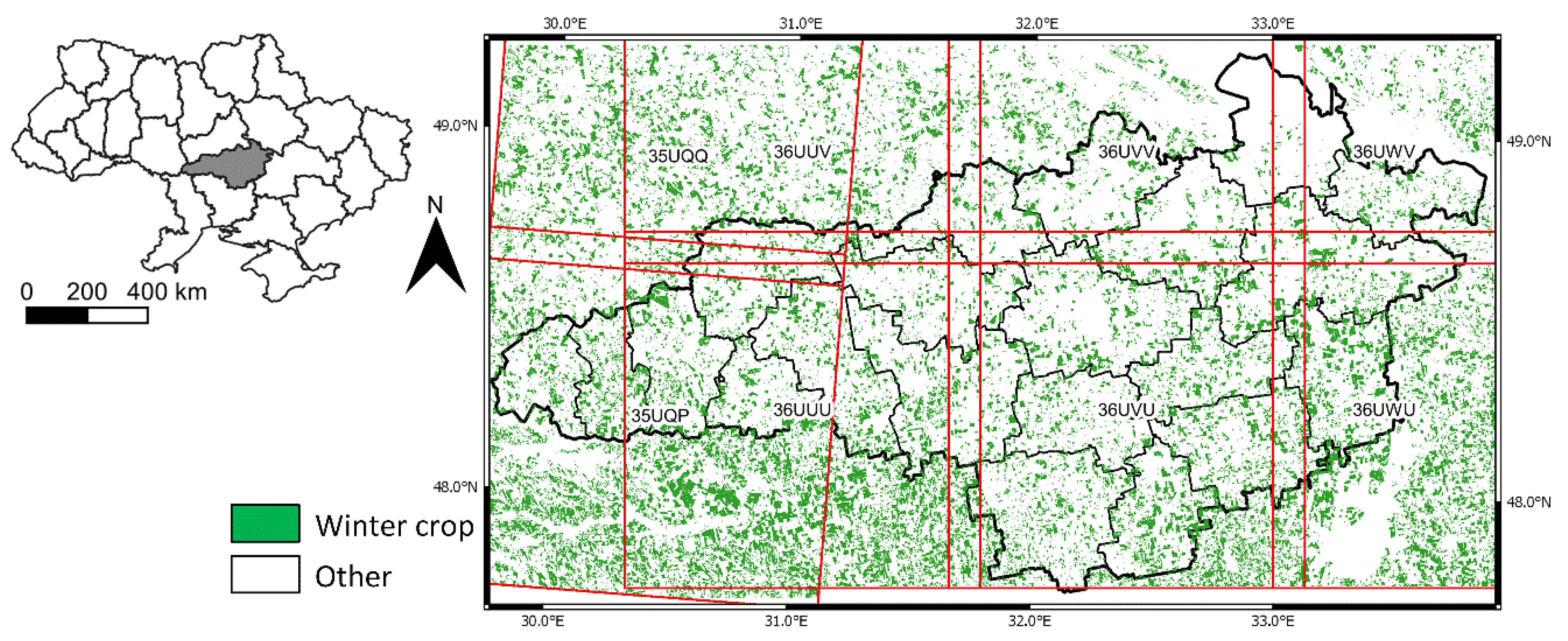
2.1. Study Area and Reference Data
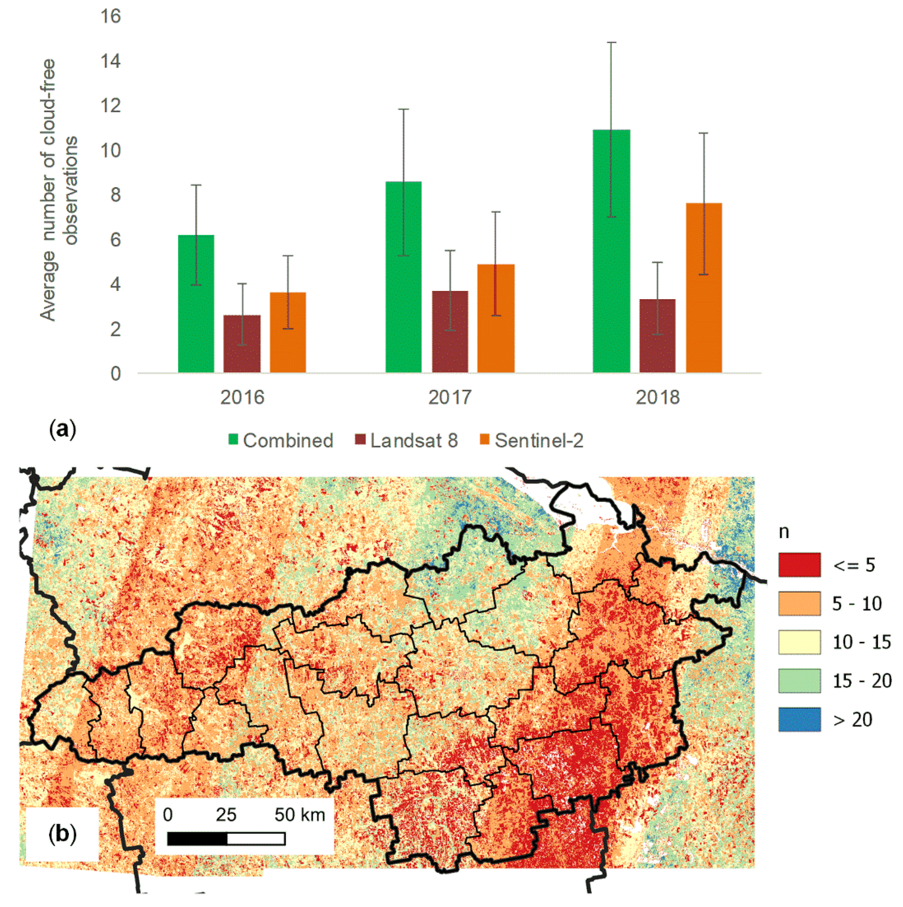
2.2. Landsat-8/OLI and Sentinel-2A /MSI Datasets
2.3. Meteorological Data
3. Methods
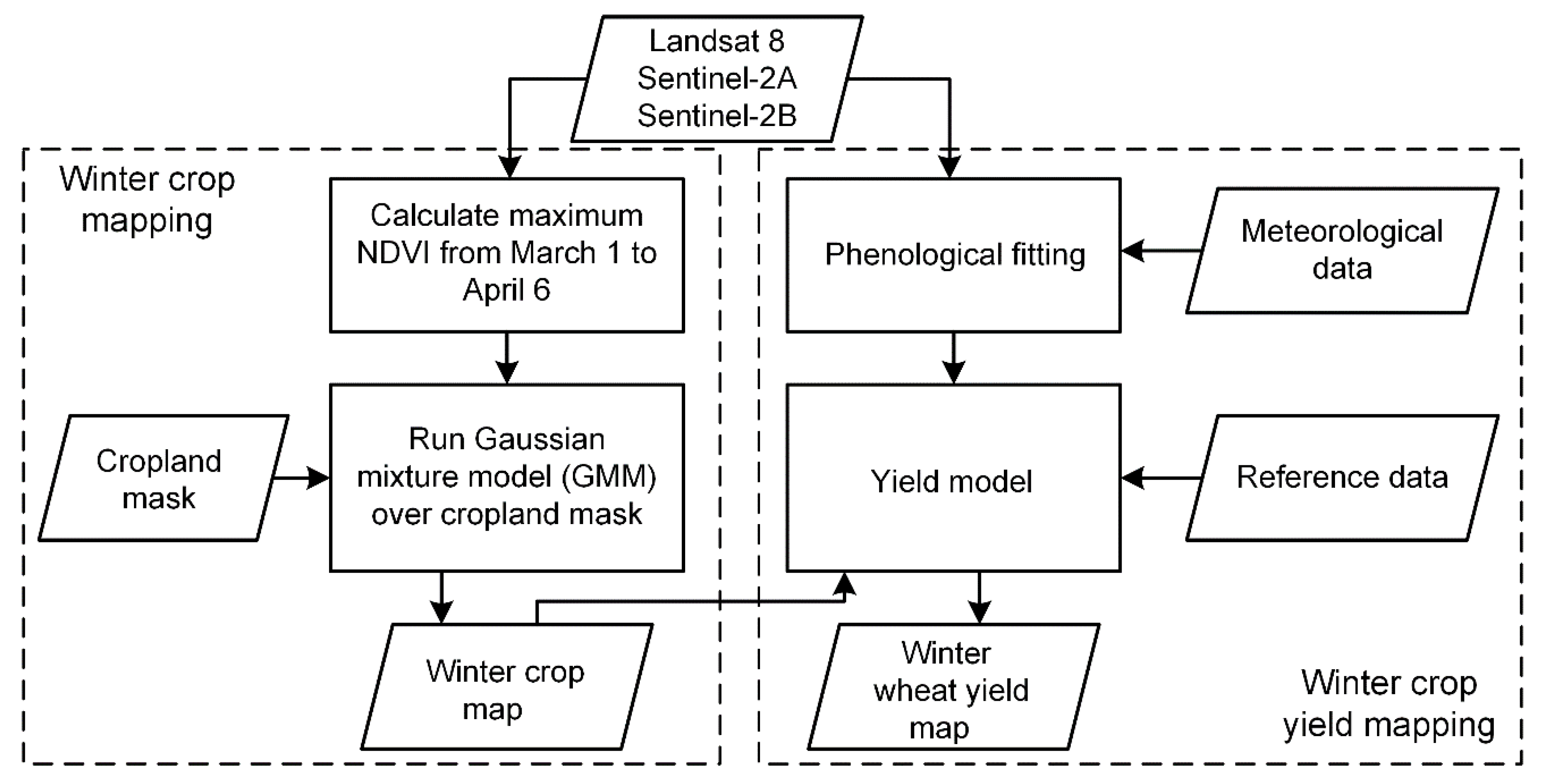
3.1. General Overview
3.2. Winter Crop Type Mapping
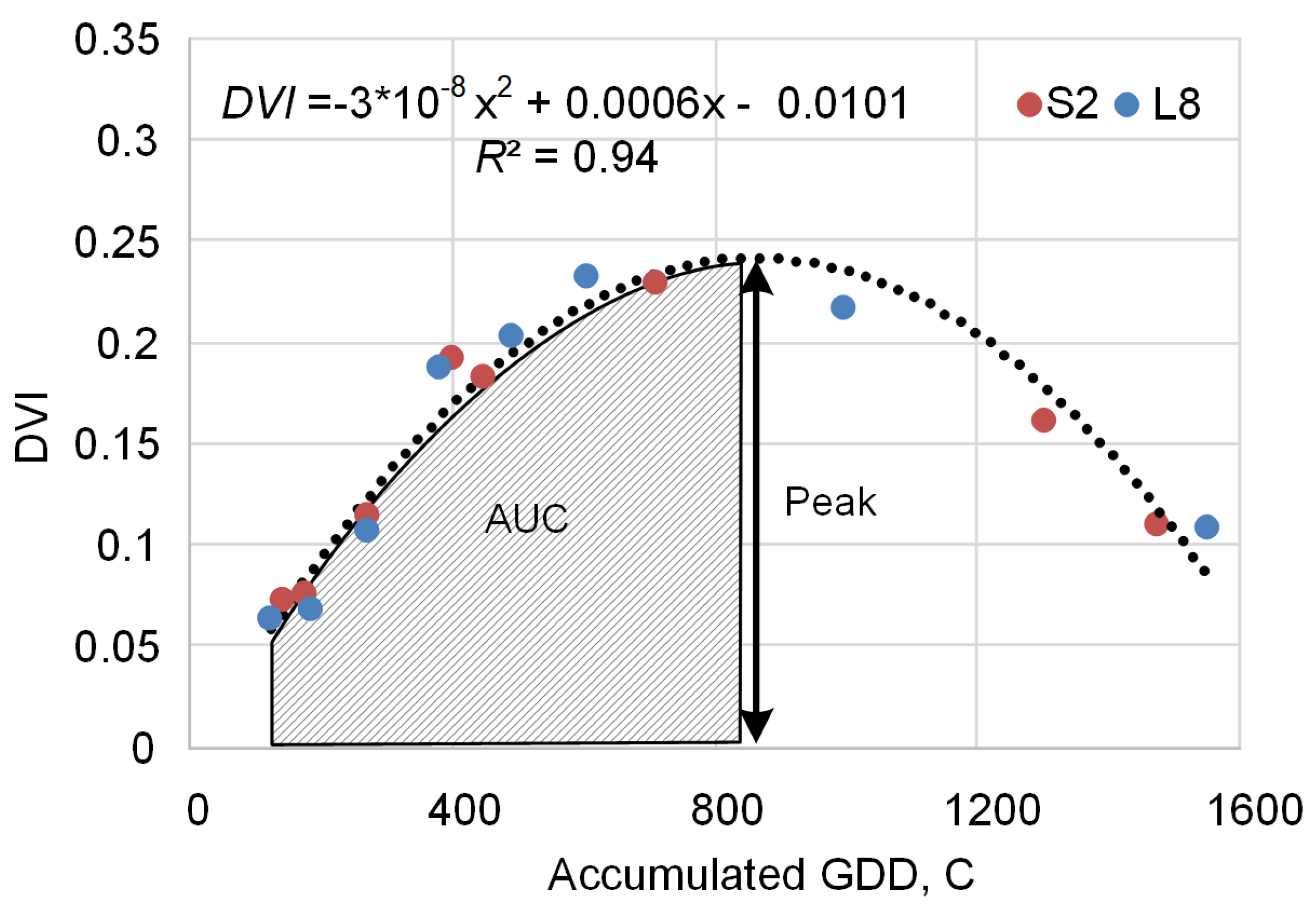
3.3. Winter Wheat Yield Assessment
3.4. Implementation and Performance Evaluation
4. Results
4.1. Winter Crop Type Mapping
4.2. Fitting VI and SR
4.3. Comparison Between VI-Based Yield Models
4.4. Impact of the Combined Use of Landsat 8 and Sentinel-2 Data
4.5. Comparison Between VI- and SR-Based Yield Models
5. Discussion
6. Conclusions
Author Contributions
Funding
Acknowledgments
Conflicts of Interest
References
- Li, J.; Roy, D.P. A Global Analysis of Sentinel-2A, Sentinel-2B and Landsat-8 Data Revisit Intervals and Implications for Terrestrial Monitoring. Remote Sens. 2017, 9, 902. [Google Scholar]
- Justice, C.O.; Vermote, E.; Townshend, J.R.; DeFries, R.; Roy, D.P.; Hall, D.K.; Salomonson, V.V.; Privette, J.L.; Riggs, G.; Strahler, A.; et al. The Moderate Resolution Imaging Spectroradiometer (MODIS): Land remote sensing for global change research. IEEE Trans. Geosci. Remote Sens. 1998, 36, 1228–1249. [Google Scholar] [CrossRef]
- Justice, C.O.; Román, M.O.; Csiszar, I.; Vermote, E.F.; Wolfe, R.E.; Hook, S.J.; Friedl, M.; Wang, Z.; Schaaf, C.B.; Miura, T.; et al. Land and cryosphere products from Suomi NPP VIIRS: Overview and status. J. Geophys. Res. Atmos. 2013, 118, 9753–9765. [Google Scholar] [CrossRef] [PubMed]
- Becker-Reshef, I.; Justice, C.; Sullivan, M.; Vermote, E.; Tucker, C.; Anyamba, A.; Small, J.; Pak, E.; Masuoka, E.; Schmaltz, J.; et al. Monitoring global croplands with coarse resolution earth observations: The Global Agriculture Monitoring (GLAM) project. Remote Sens. 2010, 2, 1589–1609. [Google Scholar] [CrossRef]
- Johnson, D.M. A comprehensive assessment of the correlations between field crop yields and commonly used MODIS products. Int. J. Appl. Earth Obs. Geoinf. 2016, 52, 65–81. [Google Scholar] [CrossRef]
- Meroni, M.; Fasbender, D.; Balaghi, R.; Dali, M.; Haffani, M.; Haythem, I.; Hooker, J.; Lahlou, M.; Lopez-Lozano, R.; Mahyou, H.; et al. Evaluating NDVI data continuity between SPOT-VEGETATION and PROBA-V missions for operational yield forecasting in North African countries. IEEE Trans. Geosci. Remote Sens. 2016, 54, 795–804. [Google Scholar] [CrossRef]
- Becker-Reshef, I.; Vermote, E.; Lindeman, M.; Justice, C. A generalized regression-based model for forecasting winter wheat yields in Kansas and Ukraine using MODIS data. Remote Sens. Environ. 2010, 114, 1312–1323. [Google Scholar] [CrossRef]
- Franch, B.; Vermote, E.F.; Becker-Reshef, I.; Claverie, M.; Huang, J.; Zhang, J.; Justice, C.; Sobrino, J.A. Improving the timeliness of winter wheat production forecast in the United States of America, Ukraine and China using MODIS data and NCAR Growing Degree Day information. Remote Sens. Environ. 2015, 161, 131–148. [Google Scholar] [CrossRef]
- Kogan, F.; Kussul, N.; Adamenko, T.; Skakun, S.; Kravchenko, O.; Kryvobok, O.; Shelestov, A.; Kolotii, A.; Kussul, O.; Lavrenyuk, A. Winter wheat yield forecasting in Ukraine based on Earth observation, meteorological data and biophysical models. Int. J. Appl. Earth Obs. Geoinf. 2013, 23, 192–203. [Google Scholar] [CrossRef]
- Whitcraft, A.K.; Becker-Reshef, I.; Killough, B.D.; Justice, C.O. Meeting earth observation requirements for global agricultural monitoring: An evaluation of the revisit capabilities of current and planned moderate resolution optical earth observing missions. Remote Sens. 2015, 7, 1482–1503. [Google Scholar] [CrossRef]
- Whitcraft, A.K.; Vermote, E.F.; Becker-Reshef, I.; Justice, C.O. Cloud cover throughout the agricultural growing season: Impacts on passive optical earth observations. Remote Sens. Environ. 2015, 156, 438–447. [Google Scholar] [CrossRef]
- Franch, B.; Vermote, E.F.; Skakun, S.; Roger, J.C.; Becker-Reshef, I.; Murphy, E.; Justice, C. Remote sensing based yield monitoring: Application to winter wheat in United States and Ukraine. Int. J. Appl. Earth Obs. Geoinf. 2019, 76, 112–127. [Google Scholar] [CrossRef]
- Kolotii, A.; Kussul, N.; Shelestov, A.; Skakun, S.; Yailymov, B.; Basarab, R.; Lavreniuk, M.; Oliinyk, T.; Ostapenko, V. Comparison of biophysical and satellite predictors for wheat yield forecasting in Ukraine. Int. Arch. Photogramm. Remote Sens. Spat. Inf. Sci. 2015, 40, 39–44. [Google Scholar] [CrossRef]
- López-Lozano, R.; Duveiller, G.; Seguini, L.; Meroni, M.; García-Condado, S.; Hooker, J.; Leo, O.; Baruth, B. Towards regional grain yield forecasting with 1km-resolution EO biophysical products: Strengths and limitations at pan-European level. Agric. For. Meteorol. 2015, 206, 12–32. [Google Scholar] [CrossRef]
- Mkhabela, M.S.; Bullock, P.; Raj, S.; Wang, S.; Yang, Y. Crop yield forecasting on the Canadian Prairies using MODIS NDVI data. Agric. For. Meteorol. 2011, 151, 385–393. [Google Scholar] [CrossRef]
- Azzari, G.; Jain, M.; Lobell, D.B. Towards fine resolution global maps of crop yields: Testing multiple methods and satellites in three countries. Remote Sens. Environ. 2017, 202, 129–141. [Google Scholar] [CrossRef]
- Gao, F.; Masek, J.; Schwaller, M.; Hall, F. On the blending of the Landsat and MODIS surface reflectance: Predicting daily Landsat surface reflectance. IEEE Trans. Geosci. Remote Sens. 2006, 44, 2207–2218. [Google Scholar]
- Gao, F.; Anderson, M.C.; Zhang, X.; Yang, Z.; Alfieri, J.G.; Kustas, W.P.; Mueller, R.; Johnson, D.M.; Prueger, J.H. Toward mapping crop progress at field scales through fusion of Landsat and MODIS imagery. Remote Sens. Environ. 2017, 188, 9–25. [Google Scholar] [CrossRef]
- Yang, Y.; Anderson, M.C.; Gao, F.; Wardlow, B.; Hain, C.R.; Otkin, J.A.; Alfieri, J.; Yang, Y.; Sun, L.; Dulaney, W. Field-scale mapping of evaporative stress indicators of crop yield: An application over Mead, NE, USA. Remote Sens. Environ. 2018, 210, 387–402. [Google Scholar] [CrossRef]
- Gao, F.; Anderson, M.; Daughtry, C.; Johnson, D. Assessing the Variability of Corn and Soybean Yields in Central Iowa Using High Spatiotemporal Resolution Multi-Satellite Imagery. Remote Sens. 2018, 10, 1489. [Google Scholar] [CrossRef]
- Herrmann, I.; Pimstein, A.; Karnieli, A.; Cohen, Y.; Alchanatis, V.; Bonfil, D.J. LAI assessment of wheat and potato crops by VENμS and Sentinel-2 bands. Remote Sens. Environ. 2011, 115, 2141–2151. [Google Scholar] [CrossRef]
- Skakun, S.; Vermote, E.; Roger, J.C.; Franch, B. Combined Use of Landsat-8 and Sentinel-2A Images for Winter Crop Mapping and Winter Wheat Yield Assessment at Regional Scale. AIMS Geosci. 2017, 3, 163–186. [Google Scholar] [CrossRef] [PubMed]
- Lambert, M.J.; Traoré, P.C.S.; Blaes, X.; Baret, P.; Defourny, P. Estimating smallholder crops production at village level from Sentinel-2 time series in Mali’s cotton belt. Remote Sens. Environ. 2018, 216, 647–657. [Google Scholar] [CrossRef]
- Lai, Y.R.; Pringle, M.J.; Kopittke, P.M.; Menzies, N.W.; Orton, T.G.; Dang, Y.P. An empirical model for prediction of wheat yield, using time-integrated Landsat NDVI. Int. J. Appl. Earth Obs. Geoinf. 2018, 72, 99–108. [Google Scholar] [CrossRef]
- Atkinson, P.M.; Jeganathan, C.; Dash, J.; Atzberger, C. Inter-comparison of four models for smoothing satellite sensor time-series data to estimate vegetation phenology. Remote Sens. Environ. 2012, 123, 400–417. [Google Scholar] [CrossRef]
- De Beurs, K.M.; Henebry, G.M. Land surface phenology, climatic variation, and institutional change: Analyzing agricultural land cover change in Kazakhstan. Remote Sens. Environ. 2004, 89, 497–509. [Google Scholar] [CrossRef]
- Fisher, J.I.; Mustard, J.F.; Vadeboncoeur, M.A. Green leaf phenology at Landsat resolution: Scaling from the field to the satellite. Remote Sens. Environ. 2006, 100, 265–279. [Google Scholar] [CrossRef]
- Ganguly, S.; Friedl, M.A.; Tan, B.; Zhang, X.; Verma, M. Land surface phenology from MODIS: Characterization of the Collection 5 global land cover dynamics product. Remote Sens. Environ. 2010, 114, 1805–1816. [Google Scholar] [CrossRef]
- Jönsson, P.; Cai, Z.; Melaas, E.; Friedl, M.A.; Eklundh, L. A Method for Robust Estimation of Vegetation Seasonality from Landsat and Sentinel-2 Time Series Data. Remote Sens. 2018, 10, 635. [Google Scholar] [CrossRef]
- Roy, D.P.; Yan, L. Robust Landsat-based crop time series modelling. Remote Sens. Environ. 2019. [Google Scholar] [CrossRef]
- Zhang, X.; Friedl, M.A.; Schaaf, C.B.; Strahler, A.H.; Hodges, J.C.; Gao, F.; Reed, B.C.; Huete, A. Monitoring vegetation phenology using MODIS. Remote Sens. Environ. 2003, 84, 471–475. [Google Scholar] [CrossRef]
- Zhang, X.; Friedl, M.A.; Schaaf, C.B. Global vegetation phenology from Moderate Resolution Imaging Spectroradiometer (MODIS): Evaluation of global patterns and comparison with in situ measurements. J. Geophys. Res. Biogeosci. 2006, 111, G04017. [Google Scholar] [CrossRef]
- Gallego, F.J.; Kussul, N.; Skakun, S.; Kravchenko, O.; Shelestov, A.; Kussul, O. Efficiency assessment of using satellite data for crop area estimation in Ukraine. Int. J. Appl. Earth Obs. Geoinf. 2014, 29, 22–30. [Google Scholar] [CrossRef]
- Roy, D.P.; Wulder, M.A.; Loveland, T.R.; Woodcock, C.E.; Allen, R.G.; Anderson, M.C.; Helder, D.; Irons, J.R.; Johnson, D.M.; Kennedy, R.; et al. Landsat-8: Science and product vision for terrestrial global change research. Remote Sens. Environ. 2014, 145, 154–172. [Google Scholar] [CrossRef]
- Drusch, M.; Del Bello, U.; Carlier, S.; Colin, O.; Fernandez, V.; Gascon, F.; Hoersch, B.; Isola, C.; Laberinti, P.; Martimort, P.; et al. Sentinel-2: ESA’s optical high-resolution mission for GMES operational services. Remote Sens. Environ. 2012, 120, 25–36. [Google Scholar] [CrossRef]
- Claverie, M.; Ju, J.; Masek, J.G.; Dungan, J.L.; Vermote, E.F.; Roger, J.C.; Skakun, S.; Justice, C. The Harmonized Landsat and Sentinel-2 surface reflectance data set. Remote Sens. Environ. 2018, 219, 145–161. [Google Scholar] [CrossRef]
- Vermote, E.; Justice, C.; Claverie, M.; Franch, B. Preliminary analysis of the performance of the Landsat 8/OLI land surface reflectance product. Remote Sens. Environ. 2016, 185, 46–56. [Google Scholar] [CrossRef]
- Doxani, G.; Vermote, E.; Roger, J.C.; Gascon, F.; Adriaensen, S.; Frantz, D.; Hagolle, O.; Hollstein, A.; Kirches, G.; Li, F.; et al. Atmospheric correction inter-comparison exercise. Remote Sens. 2018, 10, 352. [Google Scholar] [CrossRef]
- Tucker, C.J. Red and photographic infrared linear combinations for monitoring vegetation. Remote Sens. Environ. 1979, 8, 127–150. [Google Scholar] [CrossRef]
- Jiang, Z.; Huete, A.R.; Didan, K.; Miura, T. Development of a two-band enhanced vegetation index without a blue band. Remote Sens Environ. 2008, 112, 3833–3845. [Google Scholar] [CrossRef]
- Richardson, A.J.; Wiegand, C.L. Distinguishing vegetation from soil background information. Photogramm. Eng. Remote Sens. 1977, 43, 1541–1552. [Google Scholar]
- Molod, A.; Takacs, L.; Suarez, M.; Bacmeister, J. Development of the GEOS-5 atmospheric general circulation model: Evolution from MERRA to MERRA2. Geosci. Model Dev. 2015, 8, 1339–1356. [Google Scholar] [CrossRef]
- Santamaria-Artigas, A.E.; Franch, B.; Guillevic, P.; Roger, J.-C.; Vermote, E.F.; Skakun, S. Evaluation of Near-Surface Air Temperature from Reanalysis Over the United States and Ukraine: Application to Winter Wheat Yield Forecasting. IEEE J. Sel. Top. Appl. Earth Obs. Remote Sens. 2019. [Google Scholar] [CrossRef]
- Hatfield, J.L.; Prueger, J.H. Temperature extremes: Effect on plant growth and development. Weather Clim. Extrem. 2015, 10, 4–10. [Google Scholar] [CrossRef]
- Skakun, S.; Franch, B.; Vermote, E.; Roger, J.-C.; Becker-Reshef, I.; Justice, C.; Kussul, N. Early season large-area winter crop mapping using MODIS NDVI data, growing degree days information and a Gaussian mixture model. Remote Sens. Environ. 2017, 195, 244–258. [Google Scholar] [CrossRef]
- Lavreniuk, M.; Kussul, N.; Skakun, S.; Shelestov, A.; Yailymov, B. Regional retrospective high resolution land cover for Ukraine: Methodology and results. In Proceedings of the 2015 IEEE International Geoscience and Remote Sensing Symposium (IGARSS), Milan, Italy, 26–31 July 2015; IEEE: Piscataway, NJ, USA, 2015; pp. 3965–3968. [Google Scholar]
- Bishop, C.M. Pattern Recognition and Machine Learning; Springer: New York, NY, USA, 2006. [Google Scholar]
- Alemu, W.G.; Henebry, G.M. Land surface phenologies and seasonalities using cool earthlight in mid-latitude croplands. Environ. Res. Lett. 2013, 8, 045002. [Google Scholar] [CrossRef]
- McMaster, G.S.; Wilhelm, W.W. Growing degree-days: One equation, two interpretations. Agric. For. Meteorol. 1997, 87, 291–300. [Google Scholar] [CrossRef]
- Nguyen, L.H.; Joshi, D.R.; Clay, D.E.; Henebry, G.M. Characterizing land cover/land use from multiple years of Landsat and MODIS time series: A novel approach using land surface phenology modeling and random forest classifier. Remote Sens. Environ. 2018. [Google Scholar] [CrossRef]
- Sun, L.; Gao, F.; Anderson, M.; Kustas, W.; Alsina, M.; Sanchez, L.; Sams, B.; McKee, L.; Dulaney, W.; White, W.; et al. Daily mapping of 30 m LAI and NDVI for Grape yield prediction in California Vineyards. Remote Sens. 2017, 9, 317. [Google Scholar] [CrossRef]
- Manjunath, K.R.; Potdar, M.B.; Purohit, N.L. Large area operational wheat yield model development and validation based on spectral and meteorological data. Int. J. Remote Sens. 2002, 23, 3023–3038. [Google Scholar] [CrossRef]
- He, M.; Kimball, J.; Maneta, M.; Maxwell, B.; Moreno, A.; Beguería, S.; Wu, X. Regional crop gross primary productivity and yield estimation using fused Landsat-MODIS data. Remote Sens. 2018, 10, 372. [Google Scholar] [CrossRef]
- Monteith, J.L. Solar radiation and productivity in tropical ecosystems. J. Appl. Ecol. 1972, 9, 747–766. [Google Scholar] [CrossRef]
- Prince, S.D.; Goward, S.N. Global primary production: A remote sensing approach. J. Biogeogr. 1995, 815–835. [Google Scholar] [CrossRef]
- Tucker, C.J.; Holben, B.N.; Elgin, J.H., Jr.; McMurtrey, J.E., III. Relationship of spectral data to grain yield variation. Photogramm. Eng. Remote Sens. 1980, 46, 657–666. [Google Scholar]
- Hoerl, A.E.; Kennard, R.W. Ridge regression: Biased estimation for nonorthogonal problems. Technometrics 1970, 12, 55–67. [Google Scholar] [CrossRef]
- Phillips, D.L. A technique for the numerical solution of certain integral equations of the first kind. J. ACM (JACM) 1962, 9, 84–97. [Google Scholar] [CrossRef]
- Tikhonov, A.N.; Leonov, A.S.; Yagola, A.G. Nonlinear Ill-Posed Problems; Chapman & Hall: London, UK, 1998. [Google Scholar]
- Kussul, N.; Skakun, S.; Shelestov, A.; Lavreniuk, M.; Yailymov, B.; Kussul, O. Regional scale crop mapping using multi-temporal satellite imagery. Int. Arch. Photogramm. Remote Sens. Spat. Inf. Sci. 2015, 40, 45–52. [Google Scholar] [CrossRef]
- Shelestov, A.; Kolotii, A.; Skakun, S.; Baruth, B.; Lozano, R.L.; Yailymov, B. Biophysical parameters mapping within the SPOT-5 Take 5 initiative. Eur. J. Remote Sens. 2017, 50, 300–309. [Google Scholar] [CrossRef]


| Parameters | Metric | Examples | |
|---|---|---|---|
| Single VI | Peak | 1 | |
| Single VI or SR | AUC | 1 | |
| Multiple SRs | AUC | 2–4 | |
| Multiple SRs | a0, a1, a2, AUC | 4–16 |
| 2016 (47%, Total 8,207,432 Winter Crop Pixels) | ||||||
| Value | RMSE | Average ysat | R2 | |||
| av. | std. | av. | std. | av. | std. | |
| DVI | 0.016 | 0.012 | 0.184 | 0.056 | 0.94 | 0.09 |
| EVI2 | 0.025 | 0.020 | 0.393 | 0.083 | 0.94 | 0.10 |
| NDVI | 0.033 | 0.017 | 0.603 | 0.107 | 0.94 | 0.09 |
| Green | 0.005 | 0.002 | 0.053 | 0.007 | 0.61 | 0.25 |
| Red | 0.006 | 0.003 | 0.048 | 0.011 | 0.81 | 0.16 |
| NIR | 0.017 | 0.011 | 0.232 | 0.050 | 0.90 | 0.12 |
| SWIR1 | 0.015 | 0.007 | 0.181 | 0.026 | 0.76 | 0.20 |
| SWIR2 | 0.015 | 0.008 | 0.130 | 0.031 | 0.85 | 0.14 |
| 2017 (70%, Total 9,137,931 Winter Crop Pixels) | ||||||
| Value | RMSE | Average ysat | R2 | |||
| av. | std. | av. | std. | av. | std. | |
| DVI | 0.014 | 0.009 | 0.168 | 0.051 | 0.93 | 0.10 |
| EVI2 | 0.022 | 0.015 | 0.350 | 0.076 | 0.93 | 0.11 |
| NDVI | 0.027 | 0.015 | 0.578 | 0.106 | 0.94 | 0.11 |
| Green | 0.004 | 0.002 | 0.053 | 0.006 | 0.60 | 0.26 |
| Red | 0.004 | 0.002 | 0.050 | 0.011 | 0.83 | 0.19 |
| NIR | 0.014 | 0.009 | 0.219 | 0.045 | 0.91 | 0.11 |
| SWIR1 | 0.011 | 0.006 | 0.186 | 0.027 | 0.78 | 0.21 |
| SWIR2 | 0.010 | 0.007 | 0.138 | 0.032 | 0.88 | 0.15 |
| 2018 (85%, Total 10,334,332 Winter Crop Pixels) | ||||||
| Value | RMSE | Average ysat | R2 | |||
| av. | std. | av. std. | av. | std. | ||
| DVI | 0.015 | 0.010 | 0.181 | 0.059 | 0.88 | 0.13 |
| EVI2 | 0.025 | 0.016 | 0.349 | 0.089 | 0.88 | 0.13 |
| NDVI | 0.030 | 0.017 | 0.616 | 0.119 | 0.90 | 0.12 |
| Green | 0.005 | 0.002 | 0.052 | 0.007 | 0.59 | 0.27 |
| Red | 0.005 | 0.003 | 0.050 | 0.012 | 0.77 | 0.21 |
| NIR | 0.015 | 0.009 | 0.230 | 0.052 | 0.83 | 0.17 |
| SWIR1 | 0.013 | 0.007 | 0.180 | 0.030 | 0.72 | 0.24 |
| SWIR2 | 0.012 | 0.008 | 0.129 | 0.036 | 0.79 | 0.20 |
| Model | R2 | RMSE, t/ha | RRMSE, % | p-Value |
|---|---|---|---|---|
| 2016 | ||||
| Peak-DVI (data) | 0.179 | 0.308 | 7.7 | 5.61*10−2 |
| Peak-DVI (fitting) | 0.332 | 0.278 | 7.0 | 6.29*10−3 |
| AUC-DVI | 0.588 | 0.218 | 5.5 | 5.02*10−5 |
| Peak-EVI2 (data) | 0.056 | 0.330 | 8.3 | 3.03*10−1 |
| Peak-EVI2 (fitting) | 0.282 | 0.288 | 7.2 | 1.32*10−2 |
| AUC-EVI2 | 0.209 | 0.302 | 7.6 | 3.71*10−2 |
| Peak-NDVI (data) | 0.088 | 0.325 | 8.1 | 1.92*10−1 |
| Peak-NDVI (fitting) | 0.485 | 0.244 | 6.1 | 4.55*10−4 |
| AUC-NDVI | 0.057 | 0.330 | 8.3 | 2.98*10−1 |
| 2017 | ||||
| Peak-DVI (data) | 0.422 | 0.247 | 7.1 | 2.63*10−3 |
| Peak-DVI (fitting) | 0.400 | 0.252 | 7.2 | 3.67*10−3 |
| AUC-DVI | 0.589 | 0.208 | 6.0 | 1.26*10−4 |
| Peak-EVI2 (data) | 0.405 | 0.251 | 7.2 | 3.40*10−3 |
| Peak-EVI2 (fitting) | 0.381 | 0.256 | 7.3 | 4.89*10−3 |
| AUC-EVI2 | 0.570 | 0.213 | 6.1 | 1.87*10−4 |
| Peak-NDVI (data) | 0.388 | 0.254 | 7.3 | 4.38*10−3 |
| Peak-NDVI (fitting) | 0.393 | 0.253 | 7.3 | 4.05*10−3 |
| AUC-NDVI | 0.407 | 0.250 | 7.2 | 3.28*10−3 |
| 2018 | ||||
| Peak-DVI (data) | 0.597 | 0.176 | 4.7 | 4.53*10−4 |
| Peak-DVI (fitting) | 0.571 | 0.182 | 4.8 | 7.08*10−4 |
| AUC-DVI | 0.608 | 0.174 | 4.6 | 3.66*10−4 |
| Peak-EVI2 (data) | 0.565 | 0.183 | 4.9 | 7.81*10−4 |
| Peak-EVI2 (fitting) | 0.507 | 0.195 | 5.2 | 1.97*10−3 |
| AUC-EVI2 | 0.532 | 0.190 | 5.1 | 1.34*10−3 |
| Peak-NDVI (data) | 0.406 | 0.214 | 5.7 | 7.92*10−3 |
| Peak-NDVI (fitting) | 0.349 | 0.224 | 6.0 | 1.60*10−2 |
| AUC-NDVI | 0.202 | 0.248 | 6.6 | 8.07*10−2 |
| Spatial CV | Temporal CV | |||||
|---|---|---|---|---|---|---|
| Model | RMSE, t/ha | RRMSE, % | R2 | RMSE, t/ha | RRMSE, % | R2 |
| VI-based and AUC | ||||||
| AUC–DVI | 0.226 | 6.0 | 0.65 | 0.257 | 6.9 | 0.60 |
| AUC–NDVI | 0.334 | 8.9 | 0.24 | 0.408 | 10.9 | 0.15 |
| AUC–EVI2 | 0.271 | 7.2 | 0.50 | 0.323 | 8.6 | 0.45 |
| AUC–NIR | 0.226 | 6.0 | 0.65 | 0.236 | 6.3 | 0.63 |
| AUC–red | 0.396 | 10.6 | 0.18 | 0.479 | 12.8 | 0.31 |
| AUC–green | 0.368 | 9.8 | 0.10 | 0.408 | 10.9 | 0.00 |
| AUC–SWIR1 | 0.388 | 10.3 | 0.01 | 0.459 | 12.3 | 0.19 |
| SR-based and AUC | ||||||
| AUC–NIR + red | 0.229 | 6.1 | 0.64 | 0.253 | 6.7 | 0.60 |
| AUC–NIR + green | 0.229 | 6.1 | 0.64 | 0.244 | 6.5 | 0.62 |
| AUC–NIR + SWIR1 | 0.228 | 6.1 | 0.65 | 0.249 | 6.6 | 0.61 |
| AUC–red + green | 0.289 | 7.7 | 0.43 | 0.427 | 11.4 | 0.35 |
| AUC–red.+ SWIR1 | 0.337 | 9.0 | 0.24 | 0.356 | 9.5 | 0.14 |
| AUC–green + SWIR1 | 0.357 | 9.5 | 0.15 | 0.457 | 12.2 | 0.04 |
| AUC–NIR + red + green + SWIR1 | 0.237 | 6.3 | 0.62 | 0.268 | 7.1 | 0.53 |
| VI/SR-based, and a0, a1, a2, AUC | ||||||
| AUC, coefficients–DVI | 0.217 | 5.8 | 0.68 | 0.218 | 5.8 | 0.68 |
| AUC, coefficients–NDVI | 0.283 | 7.6 | 0.45 | 0.328 | 8.8 | 0.30 |
| AUC, coefficients–EVI2 | 0.272 | 7.3 | 0.50 | 0.336 | 9 | 0.38 |
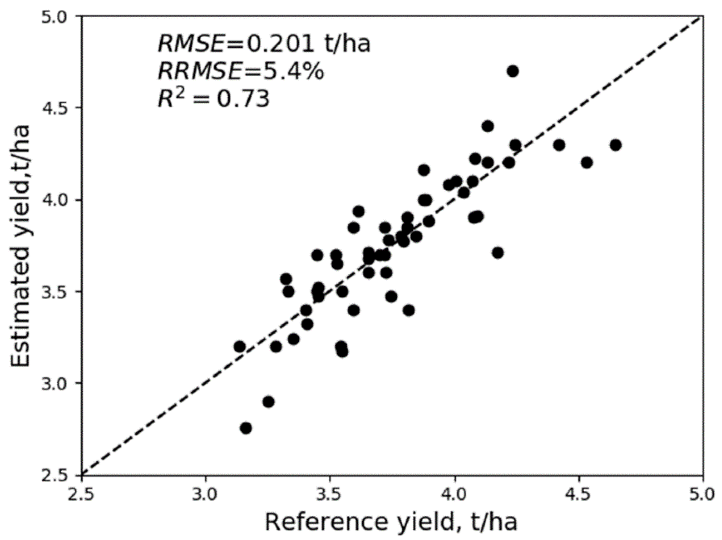
| AUC, coefficients–NIR + red | 0.207 | 5.5 | 0.71 | 0.201 | 5.4 | 0.73 |
| AUC, coefficients–NIR + green | 0.218 | 5.8 | 0.68 | 0.233 | 6.2 | 0.63 |
| AUC, coefficients–NIR + SWIR1 | 0.222 | 5.9 | 0.67 | 0.221 | 5.9 | 0.67 |
| AUC, coefficients–red + green | 0.249 | 6.6 | 0.58 | 0.366 | 9.8 | 0.53 |
| AUC, coefficients–red + SWIR1 | 0.283 | 7.6 | 0.45 | 0.291 | 7.8 | 0.43 |
| AUC, coefficients–green + SWIR1 | 0.359 | 9.6 | 0.16 | 0.486 | 13.0 | 0.03 |
| AUC, coefficients–NIR + red + green + SWIR1 | 0.212 | 5.7 | 0.70 | 0.218 | 5.8 | 0.73 |
© 2019 by the authors. Licensee MDPI, Basel, Switzerland. This article is an open access article distributed under the terms and conditions of the Creative Commons Attribution (CC BY) license (http://creativecommons.org/licenses/by/4.0/).
Share and Cite
Skakun, S.; Vermote, E.; Franch, B.; Roger, J.-C.; Kussul, N.; Ju, J.; Masek, J. Winter Wheat Yield Assessment from Landsat 8 and Sentinel-2 Data: Incorporating Surface Reflectance, Through Phenological Fitting, into Regression Yield Models. Remote Sens. 2019, 11, 1768. https://doi.org/10.3390/rs11151768
Skakun S, Vermote E, Franch B, Roger J-C, Kussul N, Ju J, Masek J. Winter Wheat Yield Assessment from Landsat 8 and Sentinel-2 Data: Incorporating Surface Reflectance, Through Phenological Fitting, into Regression Yield Models. Remote Sensing. 2019; 11(15):1768. https://doi.org/10.3390/rs11151768
Chicago/Turabian StyleSkakun, Sergii, Eric Vermote, Belen Franch, Jean-Claude Roger, Nataliia Kussul, Junchang Ju, and Jeffrey Masek. 2019. "Winter Wheat Yield Assessment from Landsat 8 and Sentinel-2 Data: Incorporating Surface Reflectance, Through Phenological Fitting, into Regression Yield Models" Remote Sensing 11, no. 15: 1768. https://doi.org/10.3390/rs11151768
APA StyleSkakun, S., Vermote, E., Franch, B., Roger, J.-C., Kussul, N., Ju, J., & Masek, J. (2019). Winter Wheat Yield Assessment from Landsat 8 and Sentinel-2 Data: Incorporating Surface Reflectance, Through Phenological Fitting, into Regression Yield Models. Remote Sensing, 11(15), 1768. https://doi.org/10.3390/rs11151768