Giving Ecological Meaning to Satellite-Derived Fire Severity Metrics across North American Forests

Abstract

Satellite-derived spectral indices such as the relativized burn ratio (RBR) allow fire severity maps to be produced in a relatively straightforward manner across multiple fires and broad spatial extents. These indices often have strong relationships with field-based measurements of fire severity, thereby justifying their widespread use in management and science. However, satellite-derived spectral indices have been criticized because their non-standardized units render them difficult to interpret relative to on-the-ground fire effects. In this study, we built a Random Forest model describing a field-based measure of fire severity, the composite burn index (CBI), as a function of multiple spectral indices, a variable representing spatial variability in climate, and latitude. CBI data primarily representing forested vegetation from 263 fires (8075 plots) across the United States and Canada were used to build the model. Overall, the model performed well, with a cross-validated R² of 0.72, though there was spatial variability in model performance. The model we produced allows for the direct mapping of CBI, which is more interpretable compared to spectral indices. Moreover, because the model and all spectral explanatory variables were produced in Google Earth Engine, predicting and mapping of CBI can realistically be undertaken on hundreds to thousands of fires. We provide all necessary code to execute the model and produce maps of CBI in Earth Engine. This study and its products will be extremely useful to managers and scientists in North America who wish to map fire effects over large landscapes or regions.

1. Introduction

Fire severity, defined here as fire-induced change to physical ecosystem components such as vegetation and soil [1,2], is a critical fire regime component that influences landscape heterogeneity, soil erosion, nutrient cycling, wildlife habitat, post-fire successional trajectories, and other ecological factors [3,4,5,6,7]. Consequently, there is great interest in mapping fire severity patterns [8,9], opportunities for which have greatly expanded with the availability of multi-spectral satellite imagery [10,11]. Satellite-derived spectral indices allow fire severity maps to be produced in a relatively straightforward manner across multiple fires and broad spatial extents [12] and have proven to be an invaluable resource for both the management and research communities. For example, satellite-derived indices have been used to evaluate temporal and spatial trends in fire severity [13,14,15,16], identify key factors driving fire severity patterns [17,18,19], and develop models to predict the potential ecological impacts of fire prior to a fire occurring [20,21].

Over the last few decades, several satellite-derived spectral indices have been developed to measure fire severity, including the delta normalized burn ratio (dNBR) [1], the relativized delta normalized burn ratio (RdNBR) [22], and the relativized burn ratio (RBR) [23]. Generally, these spectral indices are based on Landsat Thematic Mapper (TM) and Operational Land Imager (OLI) imagery, although several studies have evaluated spectral metrics produced with other sensors such as SPOT, AVIRIS, and Sentinel [24,25,26]. These indices quantify spectral differences between pre- and post-fire imagery and often have strong relationships with field-based measures of fire severity [27,28]. Most often, the spectral indices are justified as measures of fire severity through correlations with the composite burn index (CBI), an aggregated, field-based measure of severity [1], although correlations with specific ecological responses (e.g., canopy mortality, residual litter depth, crown charring) have also been used for validation [29,30]. The robust relationship between spectral fire severity indices and CBI provides strong support for their use in estimating fire effects across landscapes. However, criticisms consistently directed towards spectral fire severity indices are that their non-standardized units make them difficult to interpret in terms of on-the-ground fire effects [31,32,33] and the nonlinear relationship between field and spectral measures of fire severity complicates interpretation [34].

In an effort to provide ecological context to non-standardized fire severity spectral indices, several studies have categorized the indices into severity classes (e.g., low, moderate, and high severity) [29,35]. Although these thresholds are often based on observed relationships to field-based assessments of severity [15,28], this is not always the case [see 32]. Another viable approach to give spectral indices ecological meaning is to produce a statistical model in which a continuous field measurement of fire severity is modeled as a function of a given spectral index [27,36,37,38]. This approach allows for the direct mapping of fire effects (e.g., CBI, changes to canopy cover) [39,40,41], which is arguably more interpretable than non-standardized spectral indices. The majority of these studies produce models relating a given field-based measure of fire severity to a single spectral index e.g., [20,37].

A small but growing number of case studies suggest that fire effects can be better characterized with machine learning models than by parametric regressions because they can easily incorporate multiple explanatory variables and their interactions [41,42,43,44]. The fundamental reasoning is that different aspects of fire-induced change can be characterized by different indices, and furthermore, machine learning techniques do not require a priori knowledge of variable interactions or functional forms. Incorporating variables sensitive to differences in physiography across broad geographic regions into machine learning models may also improve characterization of fire effects, as suggested by limited evidence that the relationship between field measures of fire severity and spectral indices may differ across biophysical gradients [23,33]. Consequently, models that incorporate diverse spectral indices and biophysical covariates to describe fire effects have the potential to provide more meaningful and accurate representations of fire severity, yet there have been no comprehensive studies across broad biophysical gradients to evaluate the applicability of such models.

Google Earth Engine is a cloud-based satellite image catalog and computing environment that allows users to conduct planetary scale geospatial analyses [45]. Earth Engine is becoming a widely used tool for measuring and quantifying continental-to-global characteristics such as annual gross primary production [46] and changes in the distribution of surface water [47] and land cover [48]. Earth Engine has also been used for mapping satellite-derived fire extent [49] and fire severity [50]. Machine learning models such as Random Forest regression and classification [51] are available in Earth Engine, and as such, models can be built and executed within Earth Engine, including those describing fire severity [44]. Given adequate field data, Earth Engine has the potential to predict and map fire effects (e.g., CBI) at continental to global scales.

We have three specific objectives, the first of which is to build a Random Forest regression model describing CBI (as a continuous variable) and evaluate several spectral, geographic, and climatic variables for inclusion into the model. Second, we aim to evaluate how the interpretation of spectral indices may vary over broad climatic or geographic gradients. Third, we intend to provide a framework and distribute code that allows users to execute the Random Forest model in Earth Engine, thereby enabling rapid production of mapped CBI predictions for fires that have occurred since 1984, with the exception of fires without available pre- or post-fire imagery.

2. Materials and Methods

2.1. Composite Burn Index Field Data

The composite burn index (CBI) is a post-fire field-based measure of fire severity, usually collected one year after fire [1]. Under the CBI protocol, over 20 individual factors are rated in each of five vertically arranged strata, including (a) substrates, (b) herbs, low shrubs, and trees < 1 m in height, (c) tall shrubs and trees 1–5 m in height, (d) intermediate trees (sub-canopy, pole-sized), and (e) big trees (upper canopy, dominant or co-dominant). There are four or five factors in each strata that include newly exposed soil/rock and duff consumption (stratum a), percent of vegetation that survived the fire and percent black/brown foliage (strata b and c), and canopy mortality and char height (strata d and e). Each factor is based on visual assessments and is rated from 0–3, with zero representing no fire effects and three representing the largest degree of change. Typically, ratings are averaged for each stratum and then across all strata to arrive at an overall CBI for an entire plot [1]. The CBI protocol is sometimes modified to better reflect fire effects in certain ecosystems (e.g., boreal forest; [27]). Figure S1 shows the standard CBI form and all factors measured in each strata.

We acquired CBI data for fires with readily available fire perimeters that primarily burned forest vegetation (i.e., shrubland, grassland, and tundra fires were not evaluated) (Figure 1). To do so, we obtained publicly distributed [52,53,54] and agency (e.g., US National Park Service and Parks Canada) CBI datasets; we also requested CBI data from specific individuals who collected such data for specific projects or uses e.g., [39]. Since we opportunistically acquired data collected by other institutions and organizations, we acknowledge that some forest ecosystems may have disproportionately low or high representation in our CBI dataset (Table S1). Nevertheless, the plot data spans broad climatic and geographic gradients of the US and Canada, making our model applicable to a large proportion of North American forests. The majority of the plots, with the exception of the eastern US, can be characterized as conifer forest, though some plots represent mixed forest (conifer and deciduous), deciduous forest, and non-forest. Most plots in the eastern US represent broadleaf deciduous forest with a lesser amount of conifer forest.

Due to unique environmental settings or other phenomena, CBI data for several fires that burned forest vegetation were excluded from our analysis. For example, we excluded CBI data for seven fires in Georgia and Florida (US) because the spectral fire severity indices were affected by intermittent or ephemeral wetlands; that is, standing water was likely present in the pre- or post-fire imagery. CBI data for the Glacier Creek Fire (Alaska) were excluded since the pre-fire vegetation comprised beetle-killed spruce trees [55], and were therefore considered non-forested prior to the fire. We excluded CBI data from a handful of other fires (n = 5) whose CBI values were highly inconsistent with post-fire aerial imagery, potentially reflecting problems with the coordinates. We also excluded CBI data from an early season prescribed fire in Canada (Y-Camp). Lastly individual plots were removed if they were duplicates or had obvious issues (e.g., located well outside of the fire perimeter with a non-zero CBI).

We also accounted for two issues with the CBI data pertaining to unburned plots (CBI = 0). First, several fires had very few or no unburned field plots. Such plots are important for characterizing the spectral values of unburned pixels (or those with minimal fire effects), to adequately model CBI, and to better evaluate the models. Our goal was that the plot data for each fire comprised at least 5% of plots represented by CBI ≤ 0.25. Consequently, for those fires with <5% of the plots with CBI ≤ 0.25, we added ‘pseudo-plots’ representing CBI = 0. We produced pseudo-plots by randomly selecting unburned pixels at a distance of 200 m outside of the fire perimeter and selected the appropriate number of unburned pixels to obtain the 5% goal. Second, several CBI = 0 plots had very high spectral fire severity values; this was not expected and likely due to errors in either the plot coordinates or the CBI field data as entered. We removed CBI = 0 plots if the corresponding RBR value was greater than the 95^th percentile of randomly placed unburned pixels. Our final CBI dataset included 8075 plots covering 263 fires that burned from 1994 to 2017. Table S1 lists all fires used in our study and the source from which we obtained CBI data. For those fires that comprised multiple polygons (i.e., a complex), we considered each polygon as an independent fire for the purpose of this study.

2.2. Explanatory Variables: Spectral, Climatic, and Geographic Data

We evaluated several variables for inclusion in the model that can be characterized as spectral, climatic, or geographic (i.e., coordinates) (

Table 1. Variables evaluated for inclusion into the Random Forest model. Equations for the spectral indices are provided in the Supplementary Materials (Table S2). Note we did not evaluate dNBR or RdNBR because (1) RBR, dNBR and RdNBR were highly correlated (Pearson’s r = 0.99) (Table S3) and (2) RBR performed marginally better than dNBR and RdNBR when validated with the CBI (Table S4).

Variable Type	Variable Abbreviation	Variable Description	Citation
Spectral	RBR	Relativized burn ratio	[23]
	dEVI	Delta enhanced vegetation index	[56]
	dNDVI	Delta normalized differenced vegetation index	[57]
	dNDMI	Delta normalized differenced moisture index	[58]
	dMIRBI	Delta mid-infrared bi-spectral index	[59]
	post.NBR	Post-fire normalized burn ratio	[1]
	post.MIRBI	Post-fire mid-infrared bi-spectral index	[59]
Climatic	CWD	Climatic water deficit	[60,61]
	AET	Actual evapotranspiration	[60,61]
Geographic	Lat	Latitude (rounded to the nearest degree)	NA
	Lon	Longitude (rounded to the nearest degree)	NA

). The spectral indices were derived from combinations of various bands from Landsat TM and OLI sensors and have been previously evaluated as measures of fire severity (Table 1, Table S2). We produced the spectral indices from Landsat imagery using the Google Earth Engine cloud computing platform [45]. For each spectral variable, we used the mean compositing approach described by Parks et al. [50] to produce pre- and post-fire image composites. This approach selects all valid pixels (i.e., free of clouds, shadows, water, and snow) within a pre-specified time window (i.e., ‘image season’,

Table 2. Image season (pre- and post-fire) for different regions.

Image Season Region	Calendar Dates	Day of Year
Canada (all) and Alaska (US)	May 20–August 31	140–243
Arizona, New Mexico (US)	April 1–June 30	91–181
California, Idaho, Montana, Oregon, S. Dakota, Utah, Washington, Wyoming (US)	June 1–September 15	152–258
Florida, Kentucky, Missouri, N. Carolina, Tennessee, Virginia (US)	May 1–July 31	121–212

) for one year prior to fire for pre-fire imagery and one year after fire for post-fire imagery. If valid pixels were unavailable during the corresponding image seasons, we extended the time frame to include imagery from two years prior or post-fire, as needed. All pixels meeting our criteria were stacked and averaged on a per-pixel basis. We did not include a dNBR offset [1] as fire perimeter accuracies were variable in Canada, reducing our confidence in offsets from unburned areas. Although most of the spectral variables rely on differences between pre- and post-fire image composites, two are characterized by post-fire image composites only (Table 1).

Climatic gradients are characterized by two variables representing the climatic water balance [60], actual evapotranspiration (AET) and the climatic water deficit (CWD). Both AET and CWD were obtained from the TerraClimate dataset [61] (resolution = 4 km) and represent climatic normals spanning 1981–2010. These variables are generally considered strong controls on the distribution of vegetation types [62,63]. Geographic coordinates are simply represented by latitude and longitude, rounded to the nearest degree.

2.3. Random Forest Model

Within Earth Engine, we built and evaluated a Random Forest model describing CBI as a function of multiple variables. Our goal was to produce a parsimonious model with a reduced set of variables, with each variable contributing to the prediction of CBI. To do so, we followed the cross-validated stepwise procedure described by Parks et al. [21]. Specifically, we built an initial model with all explanatory variables (Table 1) using a five-fold cross-validation in which data from 80% of the fires were used to build the model; CBI values were predicted for the plots representing the remaining 20% of the fires. This resulted in CBI predictions for all plots in which the plot itself was not included in the model. We then calculated the coefficient of determination (i.e., the R² of a linear model between observed vs. predicted CBI) for all plots.

Next, we built subsequent Random Forest models in which each variable was iteratively removed; each of these models was validated using the identical five-fold cross-validation. If the cross-validated R² did not decrease by at least 0.005 when any given variable was removed (in some cases, the R² increased), it indicated that the variable did not contribute any unique information. As such, any individual variable that resulted in <0.005 decrease in R² when excluded from the model was permanently removed from consideration. This process was repeated (i.e., variables were removed) until all remaining variables resulted in a decrease in R² of at least 0.005 when removed from the model. This procedure resulted in a parsimonious model in which each variable provides a non-negligible contribution. We report the cross-validated R², root mean square error (RMSE), and the mean absolute error (MAE) of the final model for observed vs. predicted CBI. All predictions were produced using the test datasets from the five-fold cross validation, such that predictions were produced for independent data not used to build the models. We also report these validation statistics for various geopolitical and ecological regions, thereby providing an indication of the spatial variability in model skill.

We initially used the default Earth Engine Random Forest parameters, except for the number of trees, which we set to 500. However, initial explorations showed these Random Forest parameters overfit the relationship between CBI and the explanatory variables (Figure 2). We reduced overfitting by manipulating the minLeafPopulation parameter, which is the minimum size of a terminal node (default = 1). We set the minLeafPopulation parameter equal to:

$$\min LeafPopulation=\frac{(num.recs/75)}{num.vars}$$

(1)

where num.recs is the number of data samples and num.vars is the number of variables in the model. This equation was based on explorations using a 5-fold cross-validation; this approach substantially reduced overfitting (Figure 2).

Initial explorations also indicated that the final model was biased, in that CBI was overpredicted at low CBI values and underpredicted at high CBI values (Figure 3). This is because the model fits the mean response, and data extremes rarely represent the mean response. The bounded nature of the CBI (range: 0–3) also plays a role. Biased predictions may complicate interpretations of mapped CBI predictions, particularly when defining classes such as low- and high-severity e.g., [17,64]. For the purpose of mapping predicted CBI, we bias corrected the CBI predictions as follows:

$$CB{I}_{bc}=\left\{\begin{array}{c}((CB{I}_{pred}-1.5)\times 1.3)+1.5,CB{I}_{pred}\le 1.5\\ ((CB{I}_{pred}-1.5)\times 1.175)+1.5,CB{I}_{pred}>1.5\end{array}\right\}$$

(2)

where CBI_bc is the bias-corrected CBI prediction and CBI_pred is the predicted CBI from the Random Forest model. The initial subtraction of 1.5 centers predicted CBI at zero, the 1.3 and 1.175 multipliers provide the bias correction, and the final 1.5 addition re-centers the predictions at 1.5. When CBI_bc resulted in predictions less than zero or greater than three, they were truncated to zero and three, respectively. We defined the parameters for this bias correction by comparing histograms of the observed CBI vs. CBI_bc (Figure S2). The bias-corrected CBI better characterizes the low and high end of the CBI gradient (Figure 3). Note that all results shown in the main body of this paper do not use the bias-corrected CBI, with the exception of the mapped predictions.

2.4. Model Implementation in Earth Engine

We designed the procedure to run entirely within Google Earth Engine [45]. This includes the production of all spectral explanatory variables, executing the model, and producing mapped CBI predictions. We provide all code and a sample fire history shapefile to produce mapped CBI predictions for 10 sample fires. The code produces two CBI predictions for each fire, one without the bias correction and one with the bias correction. Interested users can easily modify the code to produce mapped CBI predictions for nearly all fires that have burned since 1984 in North American forests, with the exception of fires without available pre- or post-fire imagery. The code is available here: https://tinyurl.com/CBImodel.

2.5. Evaluating the Potential for Spatial Variability in the Relationship between CBI and Spectral Indices

Lastly, we aimed to illustrate how variability in geography and climate influences interpretation of spectral fire severity indices. To do so, we produced two generalized additive models (GAMs), one as a function of RBR and latitude and the other as a function of RBR and CWD. Latitude and CWD were chosen because the final Random Forest model (after the cross-validated variable selection procedure) included these non-spectral variables (see Results). Using each model, we then produced plots holding CBI constant at incremental values (e.g., 1.25 and 2.25) while varying RBR and latitude and RBR and CWD.

3. Results

The Random Forest model describing CBI as a continuous variable performed well across North America (Figure 4;

Table 3. Cross-validated model skill (observed vs. predicted CBI) for Random Forest regression models describing CBI as a continuous variable. Table S4 shows the results for single variable models for each spectral variable.

Variable Group	R2	RMSE	MAE
RBR only	0.68	0.51	0.40
Full model (all selected variables)	0.72	0.47	0.37

). The cross-validated R², RMSE, and MAE were 0.72, 0.47, and 0.37, respectively. The spectral variables, particularly the RBR, provided the largest contribution to the models (Table 3 and Table S4). The cross-validated stepwise procedure we used for variable selection resulted in a parsimonious Random Forest model describing CBI as a function of RBR, dMIRBI, dNDVI, post.MIRBI, CWD, and latitude. Some spectral variables (i.e., dEVI, dNDMI, post.NBR), AET, and longitude were excluded as a result of the cross-validated model selection procedure.

Spatial variability in model skill was evident (Figure 5, Figure 6 and Figure 7;

Table 4. Cross-validated model skill (observed vs. predicted CBI) for states, provinces, and territories in our study.

State/Province/ Territory	Country	Number of Fires	Number of Plots	R2	RMSE	MAE
Alaska	US	19	725	0.62	0.52	0.38
Arizona	US	32	977	0.82	0.40	0.32
Arkansas	US	1	14	0.11	0.31	0.24
California	US	62	1889	0.73	0.45	0.35
Colorado	US	2	31	0.75	0.56	0.40
Florida	US	7	232	0.01	0.53	0.44
Idaho	US	3	115	0.68	0.44	0.34
Kentucky	US	4	17	0.08	0.69	0.51
Missouri	US	4	55	0.03	0.43	0.38
Montana	US	20	565	0.73	0.44	0.35
New Mexico	US	5	192	0.79	0.44	0.34
North Carolina	US	1	4	0.00	0.57	0.47
Oregon	US	6	141	0.78	0.43	0.35
South Dakota	US	4	174	0.60	0.57	0.43
Tennessee	US	10	131	0.80	0.37	0.29
Utah	US	8	145	0.76	0.49	0.37
Virginia	US	9	170	0.54	0.48	0.39
Washington	US	13	538	0.65	0.52	0.42
Wyoming	US	22	671	0.67	0.53	0.43
Alberta	Canada	8	574	0.77	0.51	0.40
British Columbia	Canada	5	210	0.69	0.49	0.38
Manitoba	Canada	2	82	0.85	0.44	0.35
Northwest Territories	Canada	7	230	0.84	0.42	0.32
Québec	Canada	6	114	0.69	0.43	0.35
Saskatchewan	Canada	3	42	0.83	0.52	0.43
Yukon	Canada	1	37	0.86	0.64	0.56

,

Table 5. Cross-validated model skill (observed vs. predicted) for large geopolitical regions in our study. NW US: Idaho, Montana, Oregon, South Dakota, Washington, Wyoming (Alaska excluded here but shown in Table 4); SE US: Arkansas, Florida, Kentucky, Missouri, North Carolina, Tennessee, Virginia; SW US: Arizona, California, Colorado, New Mexico, Utah.

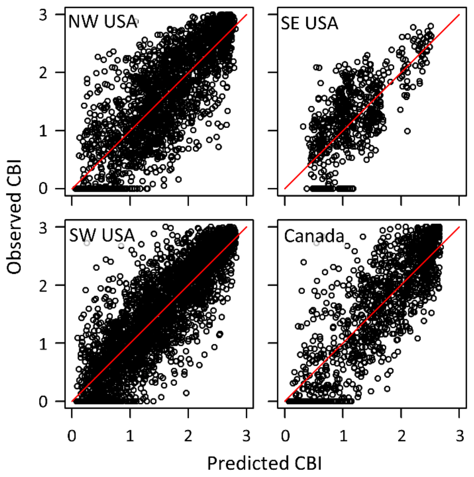
Region	Number of Fires	Number of Plots	R2	RMSE	MAE
NW US	67	2204	0.68	0.50	0.39
SE US	36	623	0.48	0.48	0.39
SW US	109	3234	0.77	0.44	0.34
Canada	32	1289	0.75	0.48	0.38

and

Table 6. Cross-validated model skill (observed vs. predicted CBI) for ecoregions (see Figure 1) in our study.

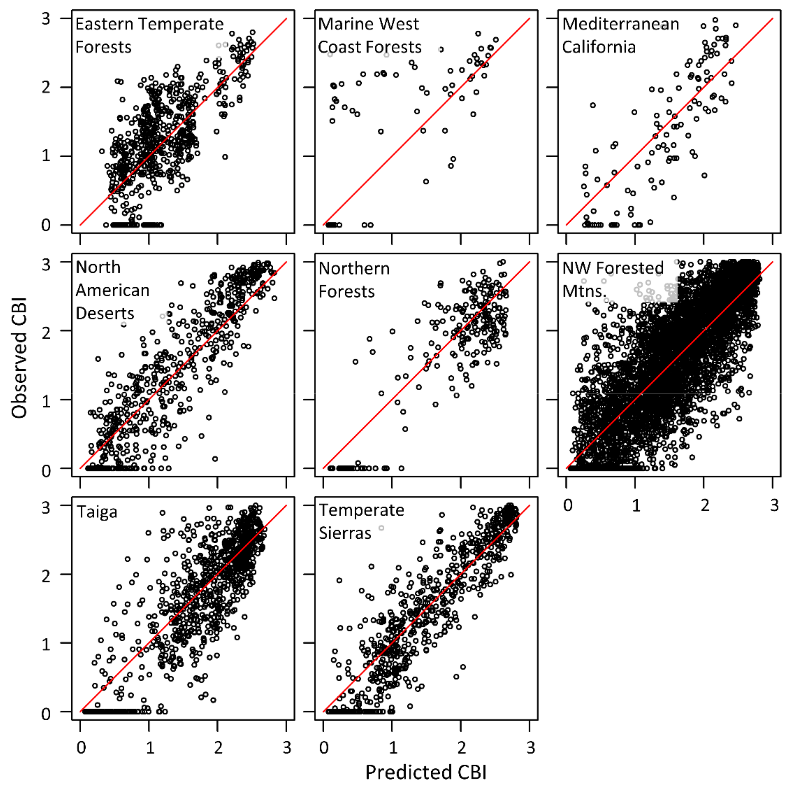
Ecoregion	Number of Fires	Number of Plots	R2	RMSE	MAE
Eastern Temperate Forests	36	623	0.48	0.48	0.39
Marine West Coast Forests	2	67	0.37	0.89	0.64
Mediterranean California	4	113	0.66	0.54	0.45
North American Deserts	28	565	0.81	0.44	0.35
Northern Forests	11	238	0.76	0.45	0.37
NW Forested Mountains	144	4882	0.72	0.48	0.38
Taiga	26	909	0.73	0.46	0.35
Temperate Sierras	26	678	0.82	0.41	0.31

). For example, CBI was modeled well (e.g., high R², low RMSE, and low MAE) in Arizona, California, New Mexico, and Alberta (Figure 5; Table 4), but our model was weaker in states such as Virginia and Alaska. Although model skill for some geopolitical units was fairly poor, small sample sizes make the validation statistics uncertain (e.g., Arkansas and North Carolina). Also, the CBI data in some geopolitical units only captured a fairly small portion of the possible CBI range, adding to the uncertainty in model skill. For example, the CBI data for Missouri spanned from 0.10 to 1.65, thereby omitting about half of the range in CBI. Issues of low sample size and inadequate sampling of the CBI gradient were mostly evident in the southeastern US. When all cross-validated CBI predictions were compared with observed CBI within broad geopolitical units, our model performed best in the southwestern US and Canada (Figure 6; Table 5) and rather poorly in the SE US. In relation to ecoregions [65], the model performed best in North American Deserts, Northern Forests, and Temperate Sierras (Figure 7; Table 6). Assessments of model skill for the bias-corrected version are provided in the Supplementary Materials (Figures S3–S5, Tables S5–S7).

The relationship between CBI and RBR varied along geographic and climatic gradients in North America. Specifically, the RBR representing specific CBI values (e.g., the threshold between low/moderate severity [CBI = 1.25] and moderate/high severity [CBI = 2.25]) increased with latitude and decreased with climatic water deficit (CWD) (Figure 8).

4. Discussion

Describing fire effects with satellite imagery is an active area of research across the globe [40,66,67]. Most of this research, however, has focused on describing fire severity with one spectral index (e.g., dNBR). The focus on a single spectral index has two important consequences. First, the de facto strategy when producing fire severity maps is to show the non-standardized index [12]; these non-standardized indices are difficult to interpret in terms of on-the-ground fire effects [36,39]. Second, there is often a failure to recognize that multiple spectral indices or other bioclimatic variables may improve models describing fire severity [33,44]. In this study, we address both limitations by a) directly modelling and mapping CBI, and b) including multiple variables into our models, thereby better describing CBI across forested landscapes in the US and Canada. Consequently, our study provides an essential refinement to mapping fire severity (as it relates to ecological impacts) across North America. Also, because we distribute code that allows users to produce mapped CBI predictions within Google Earth Engine, scientists and practitioners have the ability to map fire effects over hundreds to thousands of fires (Figure 9).

Our study showed that interpretation of spectral fire severity indices varied to some degree over bioclimatic gradients, in that RBR values corresponding to the thresholds between severity classes vary by latitude and climate (Figure 8). A possible explanation is that latitude and climate are indirect proxies for broad-scale forest type, and that interpretations of spectral indices may vary among forest types e.g., [39]. Nevertheless, our findings agree with those of Harvey et al. [33], who found that identical spectral values across latitudes corresponded with different field-measured fire effects. This finding suggests that evaluations of spectral fire severity across broad region [17,21,68] could be slightly misinterpreted without implicitly accounting for biophysical factors that influence interpretation of spectral indices. The changing interpretation between field-based fire effects and spectral indices provides ample rationale that biophysical variables should be explicitly evaluated for inclusion into models describing fire severity across broad spatial domains, as we did in this study.

The relativized burn ratio (RBR) was clearly the most important variable that we evaluated in our models (Table S4). Although we did not evaluate dNBR and RdNBR for inclusion into the model due to their very high correlation with RBR (Table S3), either would likely have been the most important variable were they used instead of RBR. The addition of other spectral variables (dMIRBI, dNDVI, post.MIRBI), CWD, and latitude provided a modest improvement compared to the model based only on RBR; the full model improved the cross-validated R² by 0.04. Although we were somewhat surprised that the improvement of the full (multi-variable) model was not greater, it could be that including additional variables results in model improvement in specific CBI ranges (e.g., low severity), as previously demonstrated [44]. Nevertheless, our study illustrates the utility of using multiple variables to model fire effects and supports the findings of several case studies to this effect [41,42,43,44].

Many studies have demonstrated that the relationship between field-based fire effects and spectral fire severity indices varies across fires and vegetation types [55,69,70]. This has led to questions as to whether or not fire severity indices, or more specifically, the functional relationships between fire effects and a spectral index, are ‘transferable’ across fires and geography [71]. Although such models may indeed be transferable to some degree [72], it is generally the case that model skill decreases when multiple fires are evaluated simultaneously due to variable functional relationships (among individual fires) between field-measured fire effects and spectral indices [23,39]. We posit that our model describing and mapping CBI increases model transferability among fires and regions. Indeed, our model performed well across North America (cross-validated R² = 0.72 for all 8075 plots) even though our study area spanned a broad gradient of the biophysical environment. This is an important outcome of our study given that it is unrealistic to collect field data on all fires and build individual models for each. This said, our models do not perform well everywhere (e.g., SE US; see Table 4, Table 5 and Table 6), but this is generally due to poor relationships between field and spectral data in certain localities and not a reflection of the model itself.

The main purpose of our study was to build a parsimonious model measuring (or estimating) fire effects (i.e., fire severity). This is a nuanced but important difference from studies that aim to explain fire effects e.g., [17]. The former aims to simply quantify the ecological impact of fire without regard to the causes or drivers, whereas the latter is intended to identify factors that control fire severity such as topography, weather, and pre-fire fuel [38,73,74,75]. Since our goal was to measure fire effects, we did not include variables such as topography that potentially drive or explain fire effects. Studies that explain fire effects can be particularly useful for identifying factors that can potentially be modified to change fire severity outcomes (e.g., fuel reduction treatments) [76] or making predictions of expected fire severity prior to a fire even occurring [20,21]. We suggest that our model that measures fire effects (i.e., CBI) can be used by other researchers as a dependent variable in models that explain fire effects. This would provide more ecological meaning and an improved interpretation when, for example, evaluating drivers of fire severity or measuring reductions in fire severity from fuel treatments.

Although our models performed well in estimating field-measured CBI across broad North American geographic and climatic gradients, there are some caveats to this approach and the resulting model. First, this model should not be used to predict CBI outside of North America because (a) the geographic and climatic variables in other regions would be outside of the range used to build the model and (b) it is not clear if the relationship between CBI and the explanatory variables are similar on other continents. CBI data from other continents could be incorporated to produce a global model or a model applicable to each continent. Second, because we purposefully omitted CBI data for those fires whose pre-fire vegetation was primarily non-forest, the applicability of our models is limited to forested ecosystems. Third, our model did not perform particularly well in the SE US (R² < 0.5), an issue not unique to our study [77]. The poor performance could be due to several factors, including that most fires in the SE US in our CBI dataset were prescribed burns that may have occurred during seasons or under conditions in which fires do not typically burn. The deciduous nature of much of SE US forests could have also posed problems in terms of the spectral signatures of different phenological states (leaf off vs. leaf on). Rapid post-fire regrowth in deciduous forests may also obscure spectral fire severity assessments. Continued study into the proper timing of pre- and post-fire imagery for describing fire severity in deciduous forests would be beneficial.

It is worth noting that the CBI itself has been criticized as an imperfect measure of fire severity [34]. For example, the CBI is a post-fire assessment in which pre-fire vegetation conditions are unknown but must be estimated [78]. The CBI is also qualitative in that each factor is visually estimated and not measured per se [79]. Furthermore, the CBI aggregates several diverse fire effects into a single index, thereby obscuring specific factors of interest [31]. Lastly, in some forest ecosystems, particular factors may be more important in describing fire severity (e.g., organic matter consumption in boreal forests), even though they are given equal weight in the CBI [80]. Nevertheless, because the CBI protocol is fairly rapid to implement (~30 min/plot) [1], two field crews can collect 50+ plots in a week (depending on transportation and hiking time), thereby enabling fairly rapid and inexpensive collection of field data that can be correlated with spectral indices or used to build models such as that described in this study. In spite of the criticisms levied towards the CBI, the consistently strong correlations between CBI and spectral indices reported in the literature are a testament to its utility in fire studies e.g., [23,25,27,38].

5. Conclusions

This study introduces a publicly available model with spectral, climatic, and geographic explanatory variables that produces gridded estimates (i.e., maps) of the composite burn index (CBI), a frequently used, field-based measure of fire severity. The ability to map across a broad geographic range was achieved through the opportunistic compilation of field-based CBI collected previously for a range of studies. The model developed in our study used data from 263 fires and covered broad gradients in the geography and climate of North America to describe the CBI. Maps of CBI produced with this model are more interpretable in terms of on-the-ground fire effects compared to non-standardized spectral indices. Since our model and the resulting maps give ecological meaning to spectral indices, they will provide managers a better understanding of fire effects. The robust relationships and the fairly high model skill in most regions suggest the resulting CBI maps will be particularly beneficial in remote regions where it is expensive and difficult to acquire field measures of severity (e.g., Alaska and the majority of Canada). This said, additional CBI plot data in underrepresented areas of the continent would likely improve model skill. The full Random Forest model provided a moderate improvement in model skill compared to the RBR-only model. This is because the interpretation of fire severity indices varies geographically [33] and, furthermore, different spectral indices complement and enhance assessments compared to use of one spectral variable alone [44]. More importantly, because we provide code to fully execute the model in Google Earth Engine, we provide managers and researchers with a tool to evaluate fire effects to support management decisions and advance ecological understanding at regional, national, and continental scales of North America. Gridded maps representing estimated CBI offers the potential to assess fire effects that may be applied to a range of user-specified natural resource applications.

References

- Key, C.H.; Benson, N.C. Landscape Assessment (LA). In FIREMON: Fire Effects Monitoring and Inventory System; Gen. Tech. Rep. RMRS-GTR-164-CD; U.S. Department of Agriculture, Forest Service, Rocky Mountain Research Station: Fort Collins, CO, USA, 2006. [Google Scholar]
- Keeley, J.E. Fire intensity, fire severity and burn severity: a brief review and suggested usage. Int. J. Wildl. Fire 2009, 18, 116–126. [Google Scholar] [CrossRef]
- Turner, M.G. Disturbance and landscape dynamics in a changing world. Ecology 2010, 91, 2833–2849. [Google Scholar] [CrossRef] [PubMed]
- McKenzie, D.; Miller, C.; Falk, D.A. The Landscape Ecology of Fire; Springer Science & Business Media: Dordrecht, The Netherlands, 2011. [Google Scholar]
- Benavides-Solorio, J.; MacDonald, L.H. Post-fire runoff and erosion from simulated rainfall on small plots, Colorado Front Range. Hydrol. Process. 2001, 15, 2931–2952. [Google Scholar] [CrossRef]
- Spigel, K.M.; Robichaud, P.R. First-year post-fire erosion rates in Bitterroot National Forest, Montana. Hydrol. Process. 2007, 21, 998–1005. [Google Scholar] [CrossRef]
- Boucher, J.; Hébert, C.; Ibarzabal, J.; Bauce, É. High conservation value forests for burn-associated saproxylic beetles: an approach for developing sustainable post-fire salvage logging in boreal forest. Insect Conserv. Divers. 2016, 9, 402–415. [Google Scholar] [CrossRef]
- Parson, A.; Robichaud, P.R.; Lewis, S.A.; Napper, C.; Clark, J.T. Field Guide for Mapping Post-Fire Soil Burn Severity; Gen. Tech. Rep. RMRS-GTR-243; U.S. Department of Agriculture, Forest Service, Rocky Mountain Research Station: Fort Collins, CO, USA, 2010; Volume 243, 49p.
- Morgan, P.; Hudak, A.T.; Wells, A.; Parks, S.A.; Baggett, L.S.; Bright, B.C.; Green, P. Multidecadal trends in area burned with high severity in the Selway-Bitterroot Wilderness Area 1880-2012. Int. J. Wildl. Fire 2017, 26, 930–943. [Google Scholar] [CrossRef]
- Miller, J.D.; Yool, S.R. Mapping forest post-fire canopy consumption in several overstory types using multi-temporal Landsat TM and ETM data. Remote Sens. Environ. 2002, 82, 481–496. [Google Scholar] [CrossRef]
- White, J.D.; Ryan, K.C.; Key, C.C.; Running, S.W. Remote Sensing of Forest Fire Severity and Vegetation Recovery. Int. J. Wildl. Fire 1996, 6, 125–136. [Google Scholar] [CrossRef]
- Eidenshink, J.C.; Schwind, B.; Brewer, K.; Zhu, Z.-L.; Quayle, B.; Howard, S.M. A project for monitoring trends in burn severity. Fire Ecol. 2007, 3, 3–21. [Google Scholar] [CrossRef]
- Miller, J.D.; Safford, H.D.; Crimmins, M.; Thode, A.E. Quantitative evidence for increasing forest fire severity in the Sierra Nevada and southern Cascade Mountains, California and Nevada, USA. Ecosystems 2009, 12, 16–32. [Google Scholar] [CrossRef]
- Whitman, E.; Batllori, E.; Parisien, M.-A.; Miller, C.; Coop, J.D.; Krawchuk, M.A.; Chong, G.W.; Haire, S.L. The climate space of fire regimes in north-western North America. J. Biogeogr. 2015, 42, 1736–1749. [Google Scholar] [CrossRef]
- Reilly, M.J.; Dunn, C.J.; Meigs, G.W.; Spies, T.A.; Kennedy, R.E.; Bailey, J.D.; Briggs, K. Contemporary patterns of fire extent and severity in forests of the Pacific Northwest, USA (1985--2010). Ecosphere 2017, 8, e01695. [Google Scholar] [CrossRef]
- Stevens, J.T.; Collins, B.M.; Miller, J.D.; North, M.P.; Stephens, S.L. Changing spatial patterns of stand-replacing fire in California conifer forests. For. Ecol. Manag. 2017, 406, 28–36. [Google Scholar] [CrossRef]
- Dillon, G.K.; Holden, Z.A.; Morgan, P.; Crimmins, M.A.; Heyerdahl, E.K.; Luce, C.H. Both topography and climate affected forest and woodland burn severity in two regions of the western US, 1984 to 2006. Ecosphere 2011, 2, art130. [Google Scholar] [CrossRef]
- Cansler, C.A.; McKenzie, D. Climate, fire size, and biophysical setting control fire severity and spatial pattern in the northern Cascade Range, USA. Ecol. Appl. 2014, 24, 1037–1056. [Google Scholar] [CrossRef] [PubMed]
- Fang, L.; Yang, J.; Zu, J.; Li, G.; Zhang, J. Quantifying influences and relative importance of fire weather, topography, and vegetation on fire size and fire severity in a Chinese boreal forest landscape. For. Ecol. Manag. 2015, 356, 2–12. [Google Scholar] [CrossRef]
- Holden, Z.A.; Morgan, P.; Evans, J.S. A predictive model of burn severity based on 20-year satellite-inferred burn severity data in a large southwestern US wilderness area. For. Ecol. Manag. 2009, 258, 2399–2406. [Google Scholar] [CrossRef]
- Parks, S.A.; Holsinger, L.M.; Panunto, M.H.; Jolly, W.M.; Dobrowski, S.Z.; Dillon, G.K. High-severity fire: evaluating its key drivers and mapping its probability across western US forests. Environ. Res. Lett. 2018, 13, 044037. [Google Scholar] [CrossRef]
- Miller, J.D.; Thode, A.E. Quantifying burn severity in a heterogeneous landscape with a relative version of the delta Normalized Burn Ratio (dNBR). Remote Sens. Environ. 2007, 109, 66–80. [Google Scholar] [CrossRef]
- Parks, S.A.; Dillon, G.K.; Miller, C. A new metric for quantifying burn severity: the relativized burn ratio. Remote Sens. 2014, 6, 1827–1844. [Google Scholar] [CrossRef]
- Fernández-Manso, A.; Fernández-Manso, O.; Quintano, C. SENTINEL-2A red-edge spectral indices suitability for discriminating burn severity. Int. J. Appl. Earth Obs. Geoinf. 2016, 50, 170–175. [Google Scholar] [CrossRef]
- Van Wagtendonk, J.W.; Root, R.R.; Key, C.H. Comparison of AVIRIS and Landsat ETM+ detection capabilities for burn severity. Remote Sens. Environ. 2004, 92, 397–408. [Google Scholar] [CrossRef]
- Chafer, C.J.; Noonan, M.; Macnaught, E. The post-fire measurement of fire severity and intensity in the Christmas 2001 Sydney wildfires. Int. J. Wildl. Fire 2004, 13, 227–240. [Google Scholar] [CrossRef]
- Whitman, E.; Parisien, M.-A.; Thompson, D.K.; Hall, R.J.; Skakun, R.S.; Flannigan, M.D. Variability and drivers of burn severity in the northwestern Canadian boreal forest. Ecosphere 2018, 9. [Google Scholar] [CrossRef]
- Miller, J.D.; Knapp, E.E.; Key, C.H.; Skinner, C.N.; Isbell, C.J.; Creasy, R.M.; Sherlock, J.W. Calibration and validation of the relative differenced Normalized Burn Ratio (RdNBR) to three measures of fire severity in the Sierra Nevada and Klamath Mountains, California, USA. Remote Sens. Environ. 2009, 113, 645–656. [Google Scholar] [CrossRef]
- Lentile, L.B.; Morgan, P.; Hudak, A.T.; Bobbitt, M.J.; Lewis, S.A.; Smith, A.; Robichaud, P. Post-fire burn severity and vegetation response following eight large wildfires across the western United States. Fire Ecol. 2007, 3, 91–108. [Google Scholar] [CrossRef]
- Hudak, A.T.; Morgan, P.; Bobbitt, M.J.; Smith, A.M.S.; Lewis, S.A.; Lentile, L.B.; Robichaud, P.R.; Clark, J.T.; McKinley, R.A. The relationship of multispectral satellite imagery to immediate fire effects. Fire Ecol. 2007, 3, 64–90. [Google Scholar] [CrossRef]
- Morgan, P.; Keane, R.E.; Dillon, G.K.; Jain, T.B.; Hudak, A.T.; Karau, E.C.; Sikkink, P.G.; Holden, Z.A.; Strand, E.K. Challenges of assessing fire and burn severity using field measures, remote sensing and modelling. Int. J. Wildl. Fire 2014, 23, 1045–1060. [Google Scholar] [CrossRef]
- Kolden, C.A.; Smith, A.M.S.; Abatzoglou, J.T. Limitations and utilisation of Monitoring Trends in Burn Severity products for assessing wildfire severity in the USA. Int. J. Wildl. Fire 2015, 24, 1023–1028. [Google Scholar] [CrossRef]
- Harvey, B.J.; Andrus, R.A.; Anderson, S.C. Incorporating biophysical gradients and uncertainty into burn severity maps in a temperate fire-prone forested region. Ecosphere 2019, in press. [Google Scholar] [CrossRef]
- Lentile, L.B.; Smith, A.M.S.; Hudak, A.T.; Morgan, P.; Bobbitt, M.J.; Lewis, S.A.; Robichaud, P.R. Remote sensing for prediction of 1-year post-fire ecosystem condition. Int. J. Wildl. Fire 2009, 18, 594–608. [Google Scholar] [CrossRef]
- Collins, B.M.; Miller, J.D.; Thode, A.E.; Kelly, M.; van Wagtendonk, J.W.; Stephens, S.L. Interactions Among Wildland Fires in a Long-Established Sierra Nevada Natural Fire Area. Ecosystems 2009, 12, 114–128. [Google Scholar] [CrossRef]
- De Santis, A.; Chuvieco, E. Burn severity estimation from remotely sensed data: Performance of simulation versus empirical models. Remote Sens. Environ. 2007, 108, 422–435. [Google Scholar] [CrossRef]
- Veraverbeke, S.; Lhermitte, S.; Verstraeten, W.W.; Goossens, R. Evaluation of pre/post-fire differenced spectral indices for assessing burn severity in a Mediterranean environment with Landsat Thematic Mapper. Int. J. Remote Sens. 2011, 32, 3521–3537. [Google Scholar] [CrossRef]
- Wimberly, M.C.; Reilly, M.J. Assessment of fire severity and species diversity in the southern Appalachians using Landsat TM and ETM+ imagery. Remote Sens. Environ. 2007, 108, 189–197. [Google Scholar] [CrossRef]
- Hall, R.J.; Freeburn, J.T.; de Groot, W.J.; Pritchard, J.M.; Lynham, T.J.; Landry, R. Remote sensing of burn severity: experience from western Canada boreal fires. Int. J. Wildl. Fire 2008, 17, 476–489. [Google Scholar] [CrossRef]
- Boucher, J.; Beaudoin, A.; Hébert, C.; Guindon, L.; Bauce, É. Assessing the potential of the differenced Normalized Burn Ratio (dNBR) for estimating burn severity in eastern Canadian boreal forests. Int. J. Wildl. Fire 2017, 26, 32–45. [Google Scholar] [CrossRef]
- Chen, X.; Vogelmann, J.E.; Rollins, M.; Ohlen, D.; Key, C.H.; Yang, L.; Huang, C.; Shi, H. Detecting post-fire burn severity and vegetation recovery using multitemporal remote sensing spectral indices and field-collected composite burn index data in a ponderosa pine forest AU - Chen, Xuexia. Int. J. Remote Sens. 2011, 32, 7905–7927. [Google Scholar] [CrossRef]
- Hultquist, C.; Chen, G.; Zhao, K. A comparison of Gaussian process regression, random forests and support vector regression for burn severity assessment in diseased forests. Remote Sens. Lett. 2014, 5, 723–732. [Google Scholar] [CrossRef]
- Brewer, K.C.; Winne, C.J.; Redmond, R.L.; Opitz, D.W.; Mangrich, M.V. Classifying and Mapping Wildfire Severity. Photogramm. Eng. Remote Sens. 2005, 71, 1311–1320. [Google Scholar] [CrossRef]
- Collins, L.; Griffioen, P.; Newell, G.; Mellor, A. The utility of Random Forests for wildfire severity mapping. Remote Sens. Environ. 2018, 216, 374–384. [Google Scholar] [CrossRef]
- Gorelick, N.; Hancher, M.; Dixon, M.; Ilyushchenko, S.; Thau, D.; Moore, R. Google Earth Engine: Planetary-scale geospatial analysis for everyone. Remote Sens. Environ. 2017, 202, 18–27. [Google Scholar] [CrossRef]
- Robinson, N.P.; Allred, B.W.; Smith, W.K.; Jones, M.O.; Moreno, A.; Erickson, T.A.; Naugle, D.E.; Running, S.W. Terrestrial primary production for the conterminous United States derived from Landsat 30 m and MODIS 250 m. Remote Sens. Ecol. Conserv. 2018, 4, 264–280. [Google Scholar] [CrossRef]
- Pekel, J.-F.; Cottam, A.; Gorelick, N.; Belward, A.S. High-resolution mapping of global surface water and its long-term changes. Nature 2016, 540, 418. [Google Scholar] [CrossRef]
- Midekisa, A.; Holl, F.; Savory, D.J.; Andrade-Pacheco, R.; Gething, P.W.; Bennett, A.; Sturrock, H.J.W. Mapping land cover change over continental Africa using Landsat and Google Earth Engine cloud computing. PLoS ONE 2017, 12, e0184926. [Google Scholar] [CrossRef] [PubMed]
- Long, T.; Zhang, Z.; He, G.; Jiao, W.; Tang, C.; Wu, B.; Zhang, X.; Wang, G.; Yin, R. 30 m Resolution Global Annual Burned Area Mapping Based on Landsat Images and Google Earth Engine. Remote Sens. 2019, 11, 489. [Google Scholar] [CrossRef]
- Parks, S.A.; Holsinger, L.M.; Voss, M.A.; Loehman, R.A.; Robinson, N.P. Mean Composite Fire Severity Metrics Computed with Google Earth Engine Offer Improved Accuracy and Expanded Mapping Potential. Remote Sens. 2018, 10, 879. [Google Scholar] [CrossRef]
- Breiman, L. Random Forests. Mach. Learn. 2001, 45, 5–32. [Google Scholar] [CrossRef]
- Key, C.H.; Benson, N.C.; Soileau, S. CBI Plot Data and Photos. Available online: https://archive.usgs.gov/archive/sites/www.nrmsc.usgs.gov/science/fire/cbi/plotdata.html (accessed on 7 December 2018).
- Sikkink, P.G.; Dillon, G.K.; Keane, R.E.; Morgan, P.; Karau, E.C.; Holden, Z.A.; Silverstein, R.P. Composite Burn Index (CBI) Data and Field Photos Collected for the FIRESEV Project, Western United States; U.S. Forest Service: Fort Collins, CO, USA, 2013.
- Picotte, J.J. Composite Burn Index (CBI) Data for the Conterminous US, Collected Between 1994 and 2018. 2019; in press. [Google Scholar]
- Murphy, K.A.; Reynolds, J.H.; Koltun, J.M. Evaluating the ability of the differenced Normalized Burn Ratio (dNBR) to predict ecologically significant burn severity in Alaskan boreal forests. Int. J. Wildl. Fire 2008, 17, 490–499. [Google Scholar] [CrossRef]
- Huete, A.; Didan, K.; Miura, T.; Rodriguez, E.P.; Gao, X.; Ferreira, L.G. Overview of the radiometric and biophysical performance of the MODIS vegetation indices. Remote Sens. Environ. 2002, 83, 195–213. [Google Scholar] [CrossRef]
- Pettorelli, N.; Vik, J.O.; Mysterud, A.; Gaillard, J.-M.; Tucker, C.J.; Stenseth, N.C. Using the satellite-derived NDVI to assess ecological responses to environmental change. Trends Ecol. Evol. 2005, 20, 503–510. [Google Scholar] [CrossRef] [PubMed]
- McDonald, A.J.; Gemmell, F.M.; Lewis, P.E. Investigation of the utility of spectral vegetation indices for determining information on coniferous forests. Remote Sens. Environ. 1998, 66, 250–272. [Google Scholar] [CrossRef]
- McCarley, T.R.; Smith, A.M.S.; Kolden, C.A.; Kreitler, J. Evaluating the Mid-Infrared Bi-spectral Index for improved assessment of low-severity fire effects in a conifer forest. Int. J. Wildl. Fire 2018, 27, 407–412. [Google Scholar] [CrossRef]
- Stephenson, N.L. Climatic control of vegetation distribution: the role of the water balance. Am. Nat. 1990, 135, 649–670. [Google Scholar] [CrossRef]
- Abatzoglou, J.T.; Dobrowski, S.Z.; Parks, S.A.; Hegewisch, K.C. TerraClimate, a high-resolution global dataset of monthly climate and climatic water balance from 1958-2015. Sci. Data 2018, 5. [Google Scholar] [CrossRef] [PubMed]
- Lutz, J.A.; van Wagtendonk, J.W.; Franklin, J.F. Climatic water deficit, tree species ranges, and climate change in Yosemite National Park. J. Biogeogr. 2010, 37, 936–950. [Google Scholar] [CrossRef]
- Stephenson, N. Actual evapotranspiration and deficit: biologically meaningful correlates of vegetation distribution across spatial scales. J. Biogeogr. 1998, 25, 855–870. [Google Scholar] [CrossRef]
- Krawchuk, M.A.; Haire, S.L.; Coop, J.; Parisien, M.-A.; Whitman, E.; Chong, G.; Miller, C. Topographic and fire weather controls of fire refugia in forested ecosystems of northwestern North America. Ecosphere 2016, 7, e01632. [Google Scholar] [CrossRef]
- Commission for Environmental Cooperation. CEC Ecological Regions of North America: Toward a Common Perspective; CEC: Montreal, QC, Canada, 1997. [Google Scholar]
- Ndalila, M.N.; Williamson, G.J.; Bowman, D.M.J.S. Geographic Patterns of Fire Severity Following an Extreme Eucalyptus Forest Fire in Southern Australia: 2013 Forcett-Dunalley Fire. Fire 2018, 1, 40. [Google Scholar] [CrossRef]
- Cardil, A.; Mola-Yudego, B.; Blázquez-Casado, Á.; González-Olabarria, J.R. Fire and burn severity assessment: Calibration of Relative Differenced Normalized Burn Ratio (RdNBR) with field data. J. Environ. Manag. 2019, 235, 342–349. [Google Scholar] [CrossRef]
- Harvey, B.J.; Donato, D.C.; Turner, M.G. Drivers and trends in landscape patterns of stand-replacing fire in forests of the US Northern Rocky Mountains (1984–2010). Landsc. Ecol. 2016, 31, 2367–2383. [Google Scholar] [CrossRef]
- Allen, J.L.; Sorbel, B. Assessing the differenced Normalized Burn Ratios ability to map burn severity in the boreal forest and tundra ecosystems of Alaska’s national parks. Int. J. Wildl. Fire 2008, 17, 463–475. [Google Scholar] [CrossRef]
- Tran, B.N.; Tanase, M.A.; Bennett, L.T.; Aponte, C. Evaluation of Spectral Indices for Assessing Fire Severity in Australian Temperate Forests. Remote Sens. 2018, 10, 1680. [Google Scholar] [CrossRef]
- Cansler, C.A.; McKenzie, D. How robust are burn severity indices when applied in a new region? Evaluation of alternate field-based and remote-sensing methods. Remote Sens. 2012, 4, 456–483. [Google Scholar] [CrossRef]
- Soverel, N.O.; Coops, N.C.; Perrakis, D.D.B.; Daniels, L.D.; Gergel, S.E. The transferability of a dNBR-derived model to predict burn severity across 10 wildland fires in western Canada. Int. J. Wildl. Fire 2011, 20, 518–531. [Google Scholar] [CrossRef]
- Keyser, A.; Westerling, A. Climate drives inter-annual variability in probability of high severity fire occurrence in the western United States. Environ. Res. Lett. 2017, 12, 065003. [Google Scholar] [CrossRef]
- Barrett, K.; McGuire, A.D.; Hoy, E.E.; Kasischke, E.S. Potential shifts in dominant forest cover in interior Alaska driven by variations in fire severity. Ecol. Appl. 2011, 21, 2380–2396. [Google Scholar] [CrossRef]
- Birch, D.S.; Morgan, P.; Kolden, C.A.; Abatzoglou, J.T.; Dillon, G.K.; Hudak, A.T.; Smith, A.M.S. Vegetation, topography and daily weather influenced burn severity in central Idaho and western Montana forests. Ecosphere 2015, 6, art17. [Google Scholar] [CrossRef]
- Stevens-Rumann, C.; Prichard, S.; Strand, E.; Morgan, P. Prior wildfires influence burn severity of subsequent large fires. Can. J. For. Res. 2016, 46, 1375–1385. [Google Scholar] [CrossRef]
- Picotte, J.J.; Robertson, K.M. Validation of remote sensing of burn severity in south-eastern US ecosystems. Int. J. Wildl. Fire 2011, 20, 453–464. [Google Scholar] [CrossRef]
- McCarley, T.R.; Kolden, C.A.; Vaillant, N.M.; Hudak, A.T.; Smith, A.M.S.; Wing, B.M.; Kellogg, B.S.; Kreitler, J. Multi-temporal LiDAR and Landsat quantification of fire-induced changes to forest structure. Remote Sens. Environ. 2017, 191, 419–432. [Google Scholar] [CrossRef]
- Lentile, L.B.; Holden, Z.A.; Smith, A.M.S.; Falkowski, M.J.; Hudak, A.T.; Morgan, P.; Lewis, S.A.; Gessler, P.E.; Benson, N.C. Remote sensing techniques to assess active fire characteristics and post-fire effects. Int. J. Wildl. Fire 2006, 15, 319–345. [Google Scholar] [CrossRef]
- Kasischke, E.S.; Turetsky, M.R.; Ottmar, R.D.; French, N.H.F.; Hoy, E.E.; Kane, E.S. Evaluation of the composite burn index for assessing fire severity in Alaskan black spruce forests. Int. J. Wildl. Fire 2008, 17, 515–526. [Google Scholar] [CrossRef]