Developing Transformation Functions for VENμS and Sentinel-2 Surface Reflectance over Israel

Abstract

Vegetation and Environmental New micro Spacecraft (VENμS) and Sentinel-2 are both ongoing earth observation missions that provide high-resolution multispectral imagery at 10 m (VENμS) and 10–20 m (Sentinel-2), at relatively high revisit frequencies (two days for VENμS and five days for Sentinel-2). Sentinel-2 provides global coverage, whereas VENμS covers selected regions, including parts of Israel. To facilitate the combination of these sensors into a unified time-series, a transformation model between them was developed using imagery from the region of interest. For this purpose, same-day acquisitions from both sensor types covering the surface reflectance over Israel, between April 2018 and November 2018, were used in this study. Transformation coefficients from VENμS to Sentinel-2 surface reflectance were produced for their overlapping spectral bands (i.e., visible, red-edge and near-infrared). The performance of these spectral transformation functions was assessed using several methods, including orthogonal distance regression (ODR), the mean absolute difference (MAD), and spectral angle mapper (SAM). Post-transformation, the value of the ODR slopes were close to unity for the transformed VENμS reflectance with Sentinel-2 reflectance, which indicates near-identity of the two datasets following the removal of systemic bias. In addition, the transformation outputs showed better spectral similarity compared to the original images, as indicated by the decrease in SAM from 0.093 to 0.071. Similarly, the MAD was reduced post-transformation in all bands (e.g., the blue band MAD decreased from 0.0238 to 0.0186, and in the NIR it decreased from 0.0491 to 0.0386). Thus, the model helps to combine the images from Sentinel-2 and VENμS into one time-series that facilitates continuous, temporally dense vegetation monitoring.

1. Introduction

We are entering a golden age of high-quality public domain earth observation (EO) data. The increase in the number of EO satellite sensors provides an opportunity to combine the images from the various sensors into a temporally dense time-series. This combination of data significantly improves the temporal resolution of EO and enhances our ability to monitor land surface changes [1,2]. Many studies have previously noted the advantageous use of information at a high spatial and temporal resolution for land cover change [3,4,5], agricultural management [6,7,8], and forest monitoring [9,10]. The availability of public-domain imagery archives on the one hand, and the development of high-performance computing systems on the other, have allowed scientists to work with large volumes of EO data for continuous monitoring and analysis of earth surface phenomena [11,12,13,14,15]. Nevertheless, this progress creates new challenges: To analyze a time-series of images acquired by different sensors, the images must undergo radiometric harmonization—i.e., the spectral differences between their corresponding bands must be minimized [16].

The most common way of integrating data from two sensors is by developing empirical transformation models [17,18,19]. Harmonizing datasets, from two different sensors, requires geometric and radiometric corrections [16]. A BDRF normalization is an important step in the radiometric correction process performed in many studies [16,19,20,21,22]. Additionally, co-registration of both datasets is important in order to minimize misregistration issues during the comparison of the image pairs [16,18,19]. These studies also emphasize the importance of using a large and representative dataset in the creation of the transformation functions [16,19,21]. Sentinel-2 and the Landsat series, for example, are public-domain optical spaceborne sensors, predominantly used for land cover monitoring. In order to combine imagery from these sensors into a unified time series, previous studies have developed transformation functions between the different Landsat sensors [17,23], and also, between Landsat ETM+ and OLI with Sentinel-2 [16,18,19,24,25,26]. Nevertheless, many studies have highlighted that the difference in reflectance is not only a function of the band response but also of the target pixels. When there is a time-lag between the acquisitions of the images, during which the land-cover changes, the resulting differences in spectral reflectance between the images are not only caused by the difference in the response of the sensors. Accordingly, this time-lag should be as small as possible, since a latent assumption in the development of the transformation models is that the bias is related to the sensor differences rather than land-cover change. In addition, the prevalent land-cover types in the images used in the model development will determine the model’s generality. Thus, the empirical models developed to integrate data from two sensors are often region-specific and less applicable to other locations [18,19,26]. Hence, regional transformation coefficients should be derived in order to combine datasets from different sensors. This paper describes the development of band transformation functions between the VENμS and Sentinel-2 satellite sensors over Israel.

VENμS is a joint satellite of the Israeli and French space agencies (ISA and CNES). Launched in August 2017, it is a near-polar sun-synchronous microsatellite at a 98° inclination, orbiting at an altitude of 720 km. The satellite has a two-day revisit time and the sensor covers a swath area of 27 km with a constant view angle. The VENμS sensor is a multispectral camera with 12 narrow spectral bands in the range of 415–910 nm. The surface reflectance product is provided at a spatial resolution of 10 m for all bands [27,28]. The major focus of the VENμS mission is vegetation monitoring (with an emphasis on precision agriculture applications that are expected to benefit from the red-edge bands [29]) and the measurement of atmospheric water vapor content and aerosol optical depth [30].

Sentinel-2 is an EO mission from The European Space Agency (ESA) Copernicus program. It includes two satellites, each equipped with a Multi-Spectral Instrument (MSI), namely Sentinel-2A (launched June 2015) and Sentinel-2B (launched March 2017). Both sun-synchronous satellites are orbiting the earth at an altitude of 786 km [31]. Sentinel-2A and Sentinel-2B have a combined revisit time of five days. The push broom MSI sensor has a 20.6° field of view covering a swath width of 290 km. MSI has 13 spectral bands with varying spatial resolution, 10 m for visible (red, blue, green) and broad near-infrared (NIR); 20 m for red-edge, narrow NIR and short-wave infrared (SWIR); and 60 m for water vapor and cirrus cloud bands. VENµS and Sentinel-2 sensors produce 10-, and 12-bit, radiometric data, respectively.

VENµS has a relatively narrow view angle compared to Sentinel-2, the latter acquiring images at nadir with a wider view angle of ±10.3° from nadir. This wider field of view may cause bidirectional reflectance effects because most of the land surface consists of non-Lambertian surfaces. For better cross-sensor calibration, bidirectional reflectance distribution effects need to be minimized. Roujean et al. [32] explained an observed the reflectance variation across the swath as the bidirectional reflectance distribution function (BRDF). Roy et al. [21] examined the directional effects on Sentinel-2 surface reflectance in overlapping regions of adjacent image tiles and concluded that the difference in reflectance due to BDRF effects may introduce significant noise for monitoring applications if the BRDF effects are not treated. Studies by Claverie et al. [33] and Roy et al. [20] reported that a single set of global BRDF coefficients has shown satisfying BRDF normalization. These global coefficients have been derived for the visible, NIR and SWIR bands [20] and the red-edge bands [22]. Claverie et al. [16] and Roy et al. [21] reported that the use of these global coefficients for the BDRF correction resulted in a stable and operationally efficient correction for Sentinel-2 data.

The above literature review suggests that a BDRF correction would be required to produce a harmonized product of VENµS and Sentinel-2 surface reflectance. Accordingly, the aim of this study was to develop a transformation model, based on near-simultaneously acquired imagery, from these sensors over Israel. The specific objectives of this study were (1) to create a harmonized (both geometrically and radiometrically corrected) surface reflectance product of VENµS and Sentinel-2 imagery by adapting protocols previously established for other sensors, (2) to derive the transformation model coefficients for the overlapping spectral bands, and (3) to assess the model performance.

2. Materials and Methods

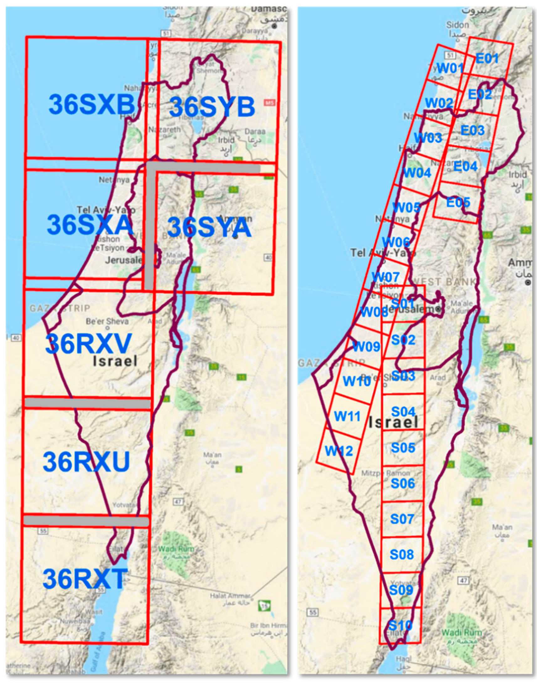
2.1. Description of the Sentinel-2 and VENµS Dataset

The state of Israel is covered by seven Sentinel-2 tiles and 27 VENµS tiles (Figure 1). As a first step, same-day acquisitions from VENµS and Sentinel-2 were inventoried. Eleven dates of near-synchronous acquisitions were found for the period from April 2018 to November 2018. In total, 77 Sentinel-2 and 230 VENµS images were used to derive the band transformation model (Table A1). Atmospherically corrected reflectance products from both sensors were used in this analysis. VENµS level-2 products were obtained from the Israel VENµS website maintained by Ben-Gurion University of the Negev (https://venus.bgu.ac.il/venus/). Sentinel-2 level-2A data were obtained from the European Space Agency’s Copernicus Open Access Hub website (https://scihub.copernicus.eu/dhus/#/home). Table 1 lists the overlapping spectral bands of the VENμS and Sentinel-2 sensors and their attributes. Figure 2 illustrates the spectral response functions of the VENμS and Sentinel-2 bands.

Figure 1. Sentinel-2 (left) and vegetation and environmental new micro spacecraft (VENμS) (right) tiles covering Israel. Tile footprints are demarked in red and their names are inscribed in blue. The grey-shaded regions in the overlap between Sentinel-2 tiles were used in the NBAR correction assessment (shown in Figure 4).

Table 1. Comparison of vegetation and environmental new micro spacecraft (VENμS) and Sentinel-2 surface reflectance products.

VENμS				Sentinel-2
	Central Wavelength (nm)	Band Width (nm)	Spatial Resolution (m)		Central Wavelength (nm)	Band Width (nm)	Spatial Resolution (m)
Band 3 (Blue)	492	40	10	Band 2 (Blue)	490	65	10
Band (Green)	555	40	10	Band 3 (Green)	560	35	10
Band 7 (Red)	666	40	10	Band 4 (Red)	665	30	10
Band 8 (Red-edge-1)	702	40	10	Band 5 (Red-edge-1)	705	15	20
Band 9 (Red-edge-2)	741	40	10	Band 6 (Red-edge-2)	740	15	20
Band 10 (Red-edge-3)	782	30	10	Band 7 (Red-edge-3)	783	20	20
Band 11 (NIR)	861	16	10	Band 8 (Broad NIR)	842	115	10
				Band 8A (Narrow NIR)	865	20	20

Figure 2. Relative spectral response functions of VENμS and Sentinel-2 bands. Sources: Sentinel-2: (ref: COPE-GSEG-EOPG-TN-15-0007) issued by European Space Agency Version 3.0, accessed from: https://earth.esa.int/web/sentinel/user-guides/sentinel-2-msi/document-library/-/asset_publisher/Wk0TKajiISaR/content/sentinel-2a-spectral-responses. VENμS: accessed from: http://www.cesbio.ups-tlse.fr/multitemp/wp-content/uploads/2018/09/rep6S.txt.

VENµS and Sentinel-2 bands were grouped into two categories based on spatial resolution (10 m and 20 m). Most of the bands preserved their native resolution, such that the original reflectance values were retained. However, the VENµS red-edge and NIR bands were resampled to 20 m to match the Sentinel-2 red-edge and narrow NIR bands.

The following considerations were made during the development of the transformation functions for Sentinel-2 and VENμS reflectance: (1) In order for the regression model input to be representative of the reflectance variance in Israel, large spatial and temporal coverages were considered; (2) the difference in reflectance values between the different sensors over non-lamebrain surfaces was corrected; (3) errors from defective or misregistered pixels were removed [25]. Figure 3 presents the steps in the development of the transformation model.

Figure 3. The processing chain for the development of transformation models between VENμS and Sentinel-2 reflectance imagery. * The VENμS red-edge bands (8–10) and near infra-red (NIR) band (11) were resampled to 20 m. ** The Sentinel-2 broad NIR and narrow NIR bands (i.e., bands 8 and 8A) were compared with the VENμS NIR band (11).

The Level-2 products used in this study were atmospherically corrected before dissemination by their respective agencies: The level-2A Sentinel-2 images were atmospherically corrected using Sentinel-2 Atmospheric Correction (S2AC) and the VENμS level-2 images were corrected using the MACCS-ATCOR Joint Algorithm (MAJA). Since these atmospherically corrected reflectance products were used to develop the transformation, atmospheric correction is not listed as a step in the process.

2.2. BRDF Correction

The BRDF correction was carried out using the c-factor technique that uses global coefficients [20,22]. Table 2 lists global coefficients that have been previously validated for Sentinel-2 and Landsat [16]. Since the VENμS bands are spectrally similar to Sentinel-2, we applied the same coefficients to the VENμS imagery. In the current work, nadir BRDF-adjusted reflectance (NBAR) values were derived for both Sentinel-2 and VENμS.

Table 2. Bidirectional reflectance distribution function (BRDF) model coefficients used in the c-factor method for the nadir BRDF-adjusted reflectance Nadir BRDF Adjusted Reflectance (NBAR) correction.

Bands	${\mathit{f}}_{\mathit{i}\mathit{s}\mathit{o}}$	${\mathit{f}}_{\mathit{g}\mathit{e}\mathit{o}}$	${\mathit{f}}_{\mathit{v}\mathit{o}\mathit{l}}$	Reference
Blue	0.0774	0.0079	0.0372	[20]
Green	0.1306	0.0178	0.058
Red	0.169	0.0227	0.0574
NIR	0.3093	0.033	0.1535
Red-edge 1	0.2085	0.0256	0.0845	[22]
Red-edge 2	0.2316	0.0273	0.1003
Red-edge 3	0.2599	0.0294	0.1197

The NBAR reflectance and c-factor were calculated as:

$$\rho \left(\lambda ,{\theta }^{NBAR}\right)=c\left(\lambda \right)\times \rho \left(\lambda ,{\theta }^{Sensor}\right)$$

(1)

$$c\left(\lambda \right)=\frac{f_{iso}\left(\lambda \right)+\left(f_{geo}\times k_{geo}\left({\theta }^{nadir}\right)\right)+\left(f_{vol}\times k_{vol}\left({\theta }^{nadir}\right)\right)}{f_{iso}\left(\lambda \right)+\left(f_{geo}\times k_{geo}\left({\theta }^{Sensor}\right)\right)+\left(f_{vol}\times k_{vol}\left({\theta }^{Sensor}\right)\right)}$$

(2)

where $\rho \left(\lambda \right)$ is the spectral reflectance for wavelength $\lambda ,$ ${\theta }^{Sensor}$ is the actual sensor’s sun-illumination geometry (i.e., angles of view zenith, sun zenith, and view-sun relative azimuth), ${\theta }^{nadir}$ is the sensor’s sun-illumination geometry at nadir position (when the view zenith angle equals zero), and $c\left(\lambda \right)$ is the correction factor for wavelength $\lambda$. $k_{vol}$ and $k_{geo}$ are the volumetric and geometric kernels and $f_{iso}$, $f_{vol}$, and $f_{geo}$ are the constant values of BRDF spectral model parameters (Table 2). The volumetric and geometric kernels are the functions defined by the view and sun illumination geometry [32]. A detailed explanation of these kernel functions is given in the theoretical document of MODIS BDRF/Albedo product [34]. In the Equation (2) nominator, the view zenith angle is set to nadir (zero) and the average value of the solar zenith angle is applied in order to normalize the VENμS and Sentinel-2 reflectance. This radiometric normalization addresses the difference in reflectance that is the result of BRDF effects.

2.3. Spatial Co-Registration and Cloud Masking

The VENμS and Sentinel-2 NBAR products were co-registered to a sub-pixel precision of <0.5 pixels (RMSE) using the AutoSync Workstation tool in ERDAS IMAGINE. A second order polynomial transformation model was used in conjunction with the nearest neighbor resampling method. Tie-points with significant bias were eliminated, while the remaining tie-points were well-distributed throughout the image space to ensure proper geometrical registration. Table 3 shows the number of tie-points used for co-registration with the corresponding RMSE values.

Table 3. Summary statistics for the co-registration tie-points used to register the VENμS and Sentinel-2 NBAR products.

	10 m		20 m
	Number of Tie-Points Per Image Pair	RMSE	Number of Tie-Points Per Image Pair	RMSE
Minimum *	15	0.14	7	0.07
Maximum	454	0.49	182	0.43
Average	150	0.27	40	0.17

* VENµS cloudy image with a very small cloud-free region.

Shadow and cloud contaminated pixels were masked out of the analysis by using scene quality information from the VENμS QTL file and the Sentinel-2 scene quality flags.

2.4. Transformation Models

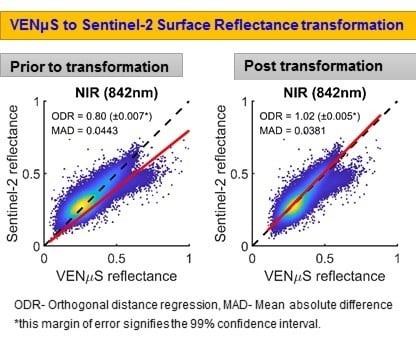
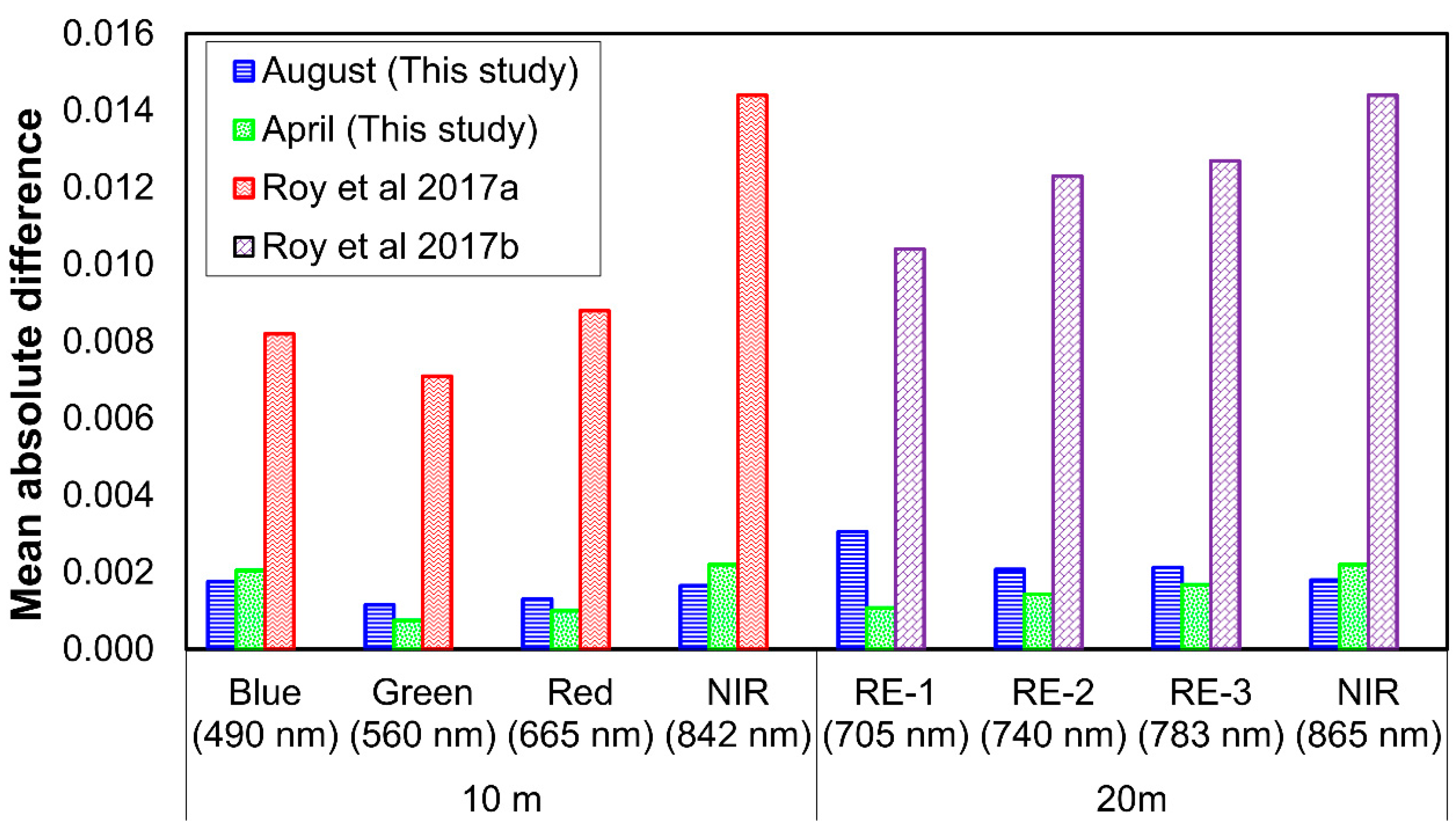
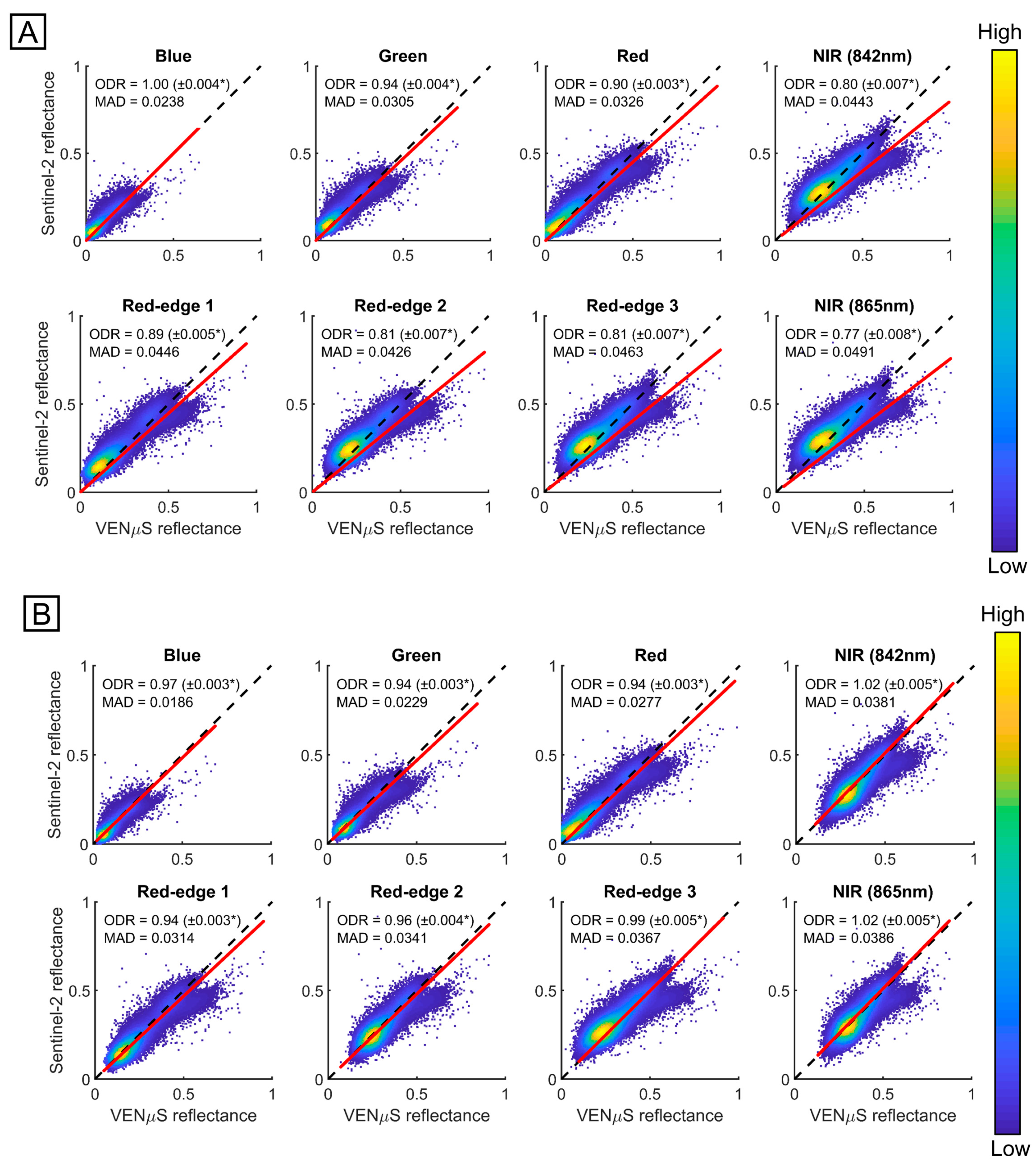
In each VENµS image, 3000–6000 random points were generated with a minimum distance of 60m between every two points. The regression model between VENμS and Sentinel-2 reflectance was produced based on 90% of these points, while the remaining 10% were used for validation. Overall, 733,562 pixels from 175 VENμS-Sentinel-2 image pairs were processed using Ordinary Least Square (OLS) regression.

$${\rho }_{Sentinel-2}=c_0+c_1{\rho }_{VEN\mu S}$$

(3)

where ${\rho }_{Sentinel-2}$ is the Sentinel-2 NBAR; ${\rho }_{VEN\mu S}$ is the VENμS NBAR; $c_0$ and $c_1$ are the OLS regression coefficients.

Since some degree of misregistration is expected, possible outliers in the dataset were removed using Cook’s distance method [35]. Cook’s distance (D_i) is defined as the sum of all the changes in the regression model when observation i is removed.

$$D_i=\frac{{{\displaystyle \sum }}_{j=1}^n{({\widehat{Y}}_j-{\widehat{Y}}_{j\left(i\right)})}^2}{\rho MSE}$$

(4)

where ${\widehat{Y}}_j$ is the jth fitted response value, ${\widehat{Y}}_{j\left(i\right)}$ is the jth fitted response value, obtained when excluding i, MSE is the mean squared error, and $\rho$ is the number of coefficients in the regression model.

The threshold used to remove the outliers in the training dataset was three times the mean Di. Values above those thresholds were removed. To remove outliers from the validation dataset, the mean Di was set as the threshold. As a result, a higher proportion of the data was removed relative to the training data. This was done to accentuate the differences in model performance—i.e., model performance using the full validation dataset (similar to the real-world data) as compared to model performance when the outliers are removed (similar to the dataset used to train the model, but slightly more refined).

Once the outliers were excluded using Cook’s distance, the final coefficients were derived based on a regression model using the remaining training pixels. These values were used to transform the VENμS reflectance in the set of validation pixels. The VENμS pixels were compared with the corresponding Sentinel-2 pixels prior to the transformation, and again post-transformation. The performance of the resulting VENμS to Sentinel-2 transformation model was subsequently assessed in three ways. First, orthogonal distance regression (ODR) was performed to assess the average proportional change between the two reflectance datasets [17]. Unlike the OLS regression, used to derive the model, the ODR slope value does not favor one variable over the other, and is only used to assess the relative divergence between the two datasets. Second, the mean absolute difference (MAD) was used to measure the difference in reflectance before and after transformation. Finally, the similarity index derived from spectral angle mapper (SAM) [36] was used to compare the reflectance values pre- and post-transformation, where smaller angle values denote higher similarity. MAD and SAM values were calculated as:

$$MAD=\frac{{\Sigma }_{i=1}^n|\left(t_i-r_i\right)|}{n}$$

(5)

where $t_i$ represents the test reflectance (i.e., reflectance values after transformation), $r_i$ denotes the reference reflectance (i.e., original reflectance values), and n represents the number of pixels considered in each band.

$$\mathrm{SAM}=\cos -1\left[\frac{{\Sigma }_{\lambda =1}^n{t}_i{r}_i}{\sqrt{{\Sigma }_{\lambda =1}^n{t}_i{}^2}\sqrt{{\Sigma }_{\lambda =1}^n{r}_i{}^2}}\right]$$

(6)

where $t_i$ represents the testing reflectance value of band i (i.e., reflectance values after transformation), $r_i$ denotes the reference reflectance (i.e., original reflectance values), and n represents the number of bands.

ODR, MAD, and SAM were only calculated for the validation set of pixels. A hypothetical perfect agreement between two sensors is expected to produce a MAD value of zero, an ODR slope of one and a SAM of zero.

3. Results

A BRDF correction was carried out for the co-acquired VENµS and Sentinel-2 imagery. The NBAR products were evaluated by comparing the Sentinel-2 NBAR reflectance images in the overlapping zones of adjacent tiles marked as grey-shaded regions in Figure 1. The mean absolute difference value for all the pairs of Sentinel-2 NBAR products was derived. To quantify the performance of the BRDF correction, the mean absolute difference found in this study was compared against previously reported values for Sentinel-2 [21,22] and our correction showed better performance (Figure 4). Accordingly, the uncertainty of this correction for Israel is significantly smaller than for the areas where this correction was originally tested.

Figure 4. Mean absolute difference between Nadir BRDF Adjusted Reflectance (NBAR) in the overlapping regions of Sentinel-2 imagery (shown in Figure 1) during the months of April and August, which represent the spring and the summer (high vegetation coverage in spring vs. low vegetation coverage in summer). The values found in this study are compared against the values reported in Roy et al. [21,22] for the month of April. RE denotes Red-edge.

The VENμS and Sentinel-2 NBAR products were co-registered with acceptable precision as shown in Table 3. In total, 733,562 training points and 89,198 validation points were randomly distributed over the imagery footprint. An example of outlier removal is shown for the green band reflectance in Figure 5. Cook’s distances that were higher than the threshold of three times the average distance were treated as outliers and excluded from the regression model (Figure 5D). The scatter plots in Figure 5A,C demonstrate the effect of outlier removal on the data distribution in the scatter plot. Table 4 presents the training and validation datasets by the band. The number of outliers for each band is slightly different because the Cook’s distance distribution is slightly different for each band.

Figure 5. Scatter plot of VENμS and Sentinel-2 green band reflectance before (A) and after (C) removing the outliers using Cook’s distance method. Subplots (B,D) show the Cook’s distance case order plot for the respective scatter plots.

Table 4. The number of points used for model training and validation. Percentage values in the brackets show the proportion of outliers excluded from the randomly created dataset using Cook’s distance method.

		Training Pixels				Validation Pixels
	Bands	Training Points (Outlier Excluded)	Outliers	Vegetation Pixels	Non-Vegetation Pixels	Validation Points (Outlier Excluded)	Outliers	Vegetation Pixels	Non-Vegetation Pixels
10 m	Blue (490 nm)	704,853	28,709 (3.9%)	251,523	453,330	78,599	10,599 (11.9%)	30,954	47,645
	Green (560 nm)	707,191	26,371 (3.6%)	254,378	452,813	79,270	9,928 (11.1%)	32,365	46,905
	Red (665 nm)	691,747	41,815 (5.7%)	246,404	445,343	77,564	11,634 (13%)	31,708	45,856
	NIR (842 nm)	707,058	26,504 (3.6%)	247,627	459,431	73,135	16,063 (18%)	28,044	45,091
20 m	Red-edge 1 (705 nm)	698,320	35,242 (4.8%)	252,604	445,716	77,093	12,105 (13.6%)	31,916	45,177
	Red-edge 2 (740 nm)	703,819	29,743 (4.1%)	250,359	453,460	75,072	14,126 (15.8%)	30,116	44,956
	Red-edge 3 (783 nm)	704,302	29,260 (4%)	247,121	457,181	73,681	15,517 (17.4%)	28,299	45,382
	NIR (865 nm)	706,113	27,449 (3.7%)	247,107	459,006	72,597	16,601 (18.6%)	27,734	44,863

Note: The initial number of pixels per band (prior to outlier removal) was 733,562 and 89,198 for the training and validation sets, respectively. Vegetation and non-vegetation pixels were grouped based on Sentinel-2 scene classification values 4 and 5. (https://earth.esa.int/web/sentinel/technical-guides/sentinel-2-msi/level-2a/algorithm).

OLS regression was performed to derive the transformation function between corresponding VENμS and Sentinel-2 bands in the visible, red-edge and NIR spectral regions. The transformation coefficients are presented in Table 5. A gradual decrease in slope, in conjunction with an increase of the intercept values, can be observed from the blue to the NIR region. Li et al. [37] also observed a similar trend for Landsat 8 to Sentinel-2 transformation. However, this trend does not appear in other Landsat and Sentinel-2 studies [16,18,19].

Table 5. Coefficients for the linear transformation from VENμS to Sentinel-2 surface reflectance.

	Bands (Central Wavelength)	Slope	ME for Slope *	Intercept	ME for Intercept *
10 m	Blue (490 nm)	1.0307	0.0010	0.0194	0.0001
	Green (560 nm)	1.0035	0.0009	0.0271	0.0002
	Red (665 nm)	0.9588	0.0007	0.0287	0.0002
	NIR (842 nm)	0.8082	0.0013	0.0768	0.0005
20m	Red-edge 1 (705 nm)	0.9589	0.0009	0.0481	0.0002
	Red-edge 2 (740 nm)	0.8632	0.0012	0.0648	0.0004
	Red-edge 3 (783 nm)	0.8347	0.0013	0.0796	0.0004
	NIR (865 nm)	0.7841	0.0013	0.0980	0.0005

Note: * ME denotes margin of error, and represents the 99% confidence interval.

Similar to the OLS regression, the pre-transformation ODR slopes in Figure 6A were in the range of 0.77 (NIR-865 nm) to 1 (blue). While the plurality of the data prior to the transformation (represented in yellow in Figure 6 and Figure 7) is centered close to the identity line, some scatter is observed in all of the bands. Figure 6B shows the scatter plots of all bands after applying the transformation by using the coefficients in Table 5. The post-transformation values of ODR slopes were all closer to 1, indicating that VENμS reflectance was transformed to become closer to Sentinel-2 reflectance. Thus, this transformation removed part of the systemic bias that is caused by the differences between the sensors.

Figure 6. Scatter plots of VENμS and Sentinel-2 surface reflectance for the validation set of pixels. (A) prior to the transformation; and (B) post-transformation. The red line is the orthogonal distance regression (ODR) slope line showing the bias relative to the identity line (black-dashed line). A high point density is marked in yellow tones, while a low point density is marked in blue tones. * This margin of error represents the 99% confidence interval.

Figure 7. Scatter plots of VENμS and Sentinel-2 surface reflectance for the validation set of pixels after the removal of outliers. (A) prior to the transformation; and (B) post-transformation. The red line is the orthogonal distance regression slope line showing the bias relative to the identity line (black dashed line). A high point density is marked in yellow tones, while a low point density is marked in blue tones. * This margin of error represents a 99% confidence interval.

The model performance was assessed for the full validation dataset following the outlier removal. Figure 7 shows the marginal improvement of the ODR slope values following the removal of outliers from the validation dataset. By lowering the Cook’s distance threshold even more, a higher proportion of data points was removed as outliers from the validation dataset compared to the training dataset. This was done to accentuate the differences between the full validation dataset and the remaining data after outlier removal. Despite the emphasis on these differences, the model coefficients did not change significantly. The ODR slopes prior to outlier removal and post-outlier removal, presented in Figure 6B and Figure 7B, respectively, show a minor change of less than 0.05. Accordingly, the coefficients given in Table 5 are expected to perform well for real-world data that contain some outliers.

The MAD values between the pre-transformed VENμS and Sentinel-2 reflectance show an increasing trend as a function of the wavelength that ranges from 0.024 (Blue) to 0.049 (NIR) for the full dataset, and 0.020 (Blue) to 0.041 (NIR) post-outlier removal. This MAD decreased post-transformation to 0.019 (Blue) and 0.039 (NIR) for the full dataset, and 0.015 (Blue) to 0.029 (NIR) post-outlier removal (Figure 8). It is evident that the transformation reduces the MAD, whether the outliers are removed or not, but that the removal of outliers further reduces the MAD. The SAM angle value for the post-transformation decreased, relative to the pre-transformed VENμS and Sentinel-2 reflectance (Figure 9). This indicates that our model transformation function increased the spectral similarity between the reflectance spectra. Therefore, the transformation developed in this paper seems to decrease systematic bias due to sensor differences, while outlier removal seems to decrease the differences by removing other sources of variation. These include atmospheric conditions that were not completely corrected, residual BRDF effects that remain untreated by the constant coefficients used in the C-factor method, and misregistration between the images.

Figure 8. Mean absolute difference (MAD) between VENμS and Sentinel-2 reflectance, prior to transformation and post-transformation.

Figure 9. Turkey box plots of the spectral angle mapper (SAM) between VENμS and Sentinel-2 reflectance (A) Full validation dataset and (B) Post removal of outliers from the dataset.

4. Discussion

In this study, we developed a transformation model for VENμS and Sentinel-2 sensors over Israel. The new model coefficients provide an opportunity to use observations at high temporal resolutions for land surface monitoring by combining Sentinel-2 and VENμS observations. The availability of the red-edge spectral bands in both sensors is significant for precision agriculture applications like irrigation management [38] and LAI assessment [29]. The same-day VENμS and Sentinel-2 image pairs were acquired during April 2018 to November 2018 and used to calibrate the transformation model. A total of eight spectral bands, namely three bands from the visible region, three red-edge bands and two from the NIR region showed an increased spectral similarity post-transformation.

The broad and narrow NIR bands of Sentinel-2 MSI were compared against the VENμS NIR band. Even though the narrow NIR has a better spectral overlap with the VENμS NIR band (Figure 2), it is not very different from the Sentinel-2 broad NIR (Figure 6, Figure 7 and Figure 8). However, Claverie et al. [16] and Li et al. [37] highlighted that the Sentinel-2 narrow NIR band has shown better performance than has the broad NIR band. Flood [18] highlighted that the difference in reflectance values of Landsat 7-ETM+ and 8-OLI for the Australian landscape was smaller than for the entire globe. In our study, more than 60 percent of the data were non-vegetated surfaces (Table 4). Thus, the transformation function developed in this study is expected to perform better for barren surfaces than for vegetation. This model can be applied for landscapes that are similar to those of Israel, i.e., Mediterranean regions. Its applicability for different environments warrants further examination.

One strength of this study is the use of near-synchronously acquired VENμS and Sentinel-2 image pairs. This minimizes changes to the land-surface, the atmosphere and sun position and, therefore, reduces any bias between the image pairs that may be caused by the temporal delay between the acquisitions of the pair of images. Accordingly, the differences between the images can largely be attributed to systematic sensor bias rather than actual changes to the ground leaving reflectance, which is expected to be minimal [18]. In this respect, this study presents an advantage over studies conducted using image pairs taken a few days apart [16,23,37].

The dissemination of a 5 m native resolution VENμS Level-2 product is expected in the near future. Mandanici and Bitelli [26] pointed out that a difference in spatial resolution can also affect the transformation function. Hence, the transformation function developed here would need to be tested to see if the change in the products’ spatial resolution has an effect, especially for the red-edge bands (VENμS-5 m to Sentinel-20 m). In addition, hyperspectral high spatial resolution imagery can be used to assess the influence of spectral resolution differences, as suggested by Claverie et al. [16] and Zhang et al. [19].

5. Conclusions

A first-of-its-kind cross-sensor calibration study for VENμS and Sentinel-2 surface reflectance data for Israel is presented. An effective processing chain that considers radiometric and geometric corrections was employed to derive the cross-sensor surface reflectance transformation model. Post-transformation, the ODR slopes were close to unity, the spectral similarity has increased as demonstrated by a reduction of the SAM value from 0.093 to 0.071, and the MAD between VENμS and Sentinel-2 reflectance was substantially decreased in all bands. This indicates that the models presented here can successfully be used to create a dense time-series of VENμS and Sentinel-2 imagery. The combined dataset of VENμS and Sentinel-2 provides high-frequency multispectral imagery that can support crop and vegetation monitoring studies, with the added advantage of red-edge bands that are absent from veteran sensors such as the Landsat series.

References

- Helder, D.; Markham, B.; Morfitt, R.; Storey, J.; Barsi, J.; Gascon, F.; Clerc, S.; LaFrance, B.; Masek, J.; Roy, D.P.; et al. Observations and Recommendations for the Calibration of Landsat 8 OLI and Sentinel 2 MSI for Improved Data Interoperability. Remote Sens. 2018, 10, 1340. [Google Scholar] [CrossRef]
- Li, J.; Roy, D.P. A Global Analysis of Sentinel-2A, Sentinel-2B and Landsat-8 Data Revisit Intervals and Implications for Terrestrial Monitoring. Remote Sens. 2017, 9, 902. [Google Scholar]
- Hansen, M.C.; Loveland, T.R. A review of large area monitoring of land cover change using Landsat data. Remote Sens. Environ. 2012, 122, 66–74. [Google Scholar] [CrossRef]
- Gómez, C.; White, J.C.; Wulder, M.A. Optical remotely sensed time series data for land cover classification: A review. ISPRS J. Photogramm. Remote Sens. 2016, 116, 55–72. [Google Scholar] [CrossRef]
- Wulder, M.A.; Coops, N.C.; Roy, D.P.; White, J.C.; Hermosilla, T. Land cover 2.0. Int. J. Remote Sens. 2018, 39, 4254–4284. [Google Scholar] [CrossRef]
- Skakun, S.; Vermote, E.; Roger, J.C.; Franch, B. Combined Use of Landsat-8 and Sentinel-2A Images for Winter Crop Mapping and Winter Wheat Yield Assessment at Regional Scale. AIMS Geosci. 2017, 3, 163–186. [Google Scholar] [CrossRef] [PubMed]
- Whitcraft, A.K.; Becker-Reshef, I.; Justice, C.O. A Framework for Defining Spatially Explicit Earth Observation Requirements for a Global Agricultural Monitoring Initiative (GEOGLAM). Remote Sens. 2015, 7, 1461–1481. [Google Scholar] [CrossRef]
- Roy, D.P.; Yan, L. Robust Landsat-based crop time series modelling. Remote Sens. Environ. (In press). [CrossRef]
- Melaas, E.K.; Friedl, M.A.; Zhu, Z. Detecting interannual variation in deciduous broadleaf forest phenology using Landsat TM/ETM+ data. Remote Sens. Environ. 2013, 132, 176–185. [Google Scholar] [CrossRef]
- Hermosilla, T.; Wulder, M.A.; White, J.C.; Coops, N.C.; Hobart, G.W.; Campbell, L.B. Mass data processing of time series Landsat imagery: Pixels to data products for forest monitoring. Int. J. Digit. Earth 2016, 9, 1035–1054. [Google Scholar] [CrossRef]
- Loveland, T.R.; Dwyer, J.L. Landsat: Building a strong future. Remote Sens. Environ. 2012, 122, 22–29. [Google Scholar] [CrossRef]
- Wulder, M.A.; Masek, J.G.; Cohen, W.B.; Loveland, T.R.; Woodcock, C.E. Opening the archive: How free data has enabled the science and monitoring promise of Landsat. Remote Sens. Environ. 2012, 122, 2–10. [Google Scholar] [CrossRef]
- Roy, D.P.; Wulder, M.A.; Loveland, T.R.; Woodcock, C.E.; Allen, R.G.; Anderson, M.C.; Helder, D.; Irons, J.R.; Johnson, D.M.; Kennedy, R.; et al. Landsat-8: Science and product vision for terrestrial global change research. Remote Sens. Environ. 2014, 145, 154–172. [Google Scholar] [CrossRef]
- Gorelick, N.; Hancher, M.; Dixon, M.; Ilyushchenko, S.; Thau, D.; Moore, R. Google Earth Engine: Planetary-scale geospatial analysis for everyone. Remote Sens. Environ. 2017, 202, 18–27. [Google Scholar] [CrossRef]
- Shelestov, A.; Lavreniuk, M.; Kussul, N.; Novikov, A.; Skakun, S. Exploring Google Earth Engine Platform for Big Data Processing: Classification of Multi-Temporal Satellite Imagery for Crop Mapping. Front. Earth Sci. 2017, 5, 17. [Google Scholar] [CrossRef]
- Claverie, M.; Ju, J.; Masek, J.G.; Dungan, J.L.; Vermote, E.F.; Roger, J.-C.; Skakun, S.V.; Justice, C. The Harmonized Landsat and Sentinel-2 surface reflectance data set. Remote Sens. Environ. 2018, 219, 145–161. [Google Scholar] [CrossRef]
- Flood, N. Continuity of Reflectance Data between Landsat-7 ETM+ and Landsat-8 OLI, for Both Top-of-Atmosphere and Surface Reflectance: A Study in the Australian Landscape. Remote Sens. 2014, 6, 7952–7970. [Google Scholar] [CrossRef]
- Flood, N. Comparing Sentinel-2A and Landsat 7 and 8 using surface reflectance over Australia. Remote Sens. 2017, 9, 659. [Google Scholar] [CrossRef]
- Zhang, H.K.; Roy, D.P.; Yan, L.; Li, Z.; Huang, H.; Vermote, E.; Skakun, S.; Roger, J.C. Characterization of Sentinel-2A and Landsat-8 top of atmosphere, surface, and nadir BRDF adjusted reflectance and NDVI differences. Remote Sens. Environ. 2018, 215, 482–494. [Google Scholar] [CrossRef]
- Roy, D.P.; Zhang, H.K.; Ju, J.; Gomez-Dans, J.L.; Lewis, P.E.; Schaaf, C.B.; Sun, Q.; Li, J.; Huang, H.; Kovalskyy, V. A general method to normalize Landsat reflectance data to nadir BRDF adjusted reflectance. Remote Sens. Environ. 2016, 176, 255–271. [Google Scholar] [CrossRef]
- Roy, D.P.; Li, J.; Zhang, H.K.; Yan, L.; Huang, H.; Li, Z. Examination of Sentinel-2A multi-spectral instrument (MSI) reflectance anisotropy and the suitability of a general method to normalize MSI reflectance to nadir BRDF adjusted reflectance. Remote Sens. Environ. 2017, 199, 25–38. [Google Scholar] [CrossRef]
- Roy, D.P.; Li, Z.; Zhang, H.K. Adjustment of Sentinel-2 Multi-Spectral Instrument (MSI) Red-Edge Band Reflectance to Nadir BRDF Adjusted Reflectance (NBAR) and Quantification of Red-Edge Band BRDF Effects. Remote Sens. 2017, 9, 1325. [Google Scholar]
- Li, P.; Jiang, L.; Feng, Z. Cross-Comparison of Vegetation Indices Derived from Landsat-7 Enhanced Thematic Mapper Plus (ETM+) and Landsat-8 Operational Land Imager (OLI) Sensors. Remote Sens. 2014, 6, 310–329. [Google Scholar] [CrossRef]
- Arekhi, M.; Goksel, C.; Sanli, F.B.; Senel, G. Comparative Evaluation of the Spectral and Spatial Consistency of Sentinel-2 and Landsat-8 OLI Data for Igneada Longos Forest. ISPRS Int. J. Geo Inf. 2019, 8, 56. [Google Scholar] [CrossRef]
- Chastain, R.; Housman, I.; Goldstein, J.; Finco, M. Empirical cross sensor comparison of Sentinel-2A and 2B MSI, Landsat-8 OLI, and Landsat-7 ETM+ top of atmosphere spectral characteristics over the conterminous United States. Remote Sens. Environ. 2019, 221, 274–285. [Google Scholar] [CrossRef]
- Mandanici, E.; Bitelli, G. Preliminary Comparison of Sentinel-2 and Landsat 8 Imagery for a Combined Use. Remote Sens. 2016, 8, 1014. [Google Scholar] [CrossRef]
- Dedieu, G.; Karnieli, A.; Hagolle, O.; Jeanjean, H.; Cabot, F.; Ferrier, P.; Yaniv, Y. VENµS: A Joint French Israeli Earth Observation Scientific Mission with High Spatial and Temporal Resolution Capabilities. In Proceedings of the 2nd International Symposium on Recent Advances in Qualitative Remote Sensing, Torrent, Spain, 25–29 September2006; pp. 517–521. [Google Scholar]
- Herscovitz, J.; Karnieli, A. VENµS program: Broad and New Horizons for Super-Spectral Imaging and Electric Propulsion Missions for a Small Satellite. In Proceedings of the AIAA/USU Conference on Small Satellites, Coming Attractions, SSC08-III-1, Logan, CO, USA, 10–13 August 2008. [Google Scholar]
- Herrmann, I.; Pimstein, A.; Karnieli, A.; Cohen, Y.; Alchanatis, V.; Bonfil, D.J. LAI assessment of wheat and potato crops by VENμS and Sentinel-2 bands. Remote Sens. Environ. 2011, 115, 2141–2151. [Google Scholar] [CrossRef]
- Hagolle, O.; Huc, M.; Pascual, D.V.; Dedieu, G. A multi-temporal method for cloud detection, applied to FORMOSAT-2, VENμS, LANDSAT and SENTINEL-2 images. Remote Sens. Environ. 2010, 114, 1747–1755. [Google Scholar] [CrossRef]
- Drusch, M.; Del Bello, U.; Carlier, S.; Colin, O.; Fernandez, V.; Gascon, F.; Hoersch, B.; Isola, C.; Laberinti, P.; Martimort, P.; et al. Sentinel-2: ESA’s Optical High-Resolution Mission for GMES Operational Services. Remote Sens. Environ. 2012, 120, 25–36. [Google Scholar] [CrossRef]
- Roujean, J.L.; Leroy, M.; Deschamps, P.Y. A Bidirectional Reflectance Model of the Earth’s Surface for the Correction of Remote Sensing Data. J. Geophys. Res. 1992, 97, 20455–20468. [Google Scholar] [CrossRef]
- Claverie, M.; Vermote, E.; Franch, B.; He, T.; Hagolle, O.; Kadiri, M.; Masek, J. Evaluation of Medium Spatial Resolution BRDF-Adjustment Techniques Using Multi-Angular SPOT4 (Take5) Acquisitions. Remote Sens. 2015, 7, 12057–12075. [Google Scholar] [CrossRef]
- Strahler, A.H.; Lucht, W.; Schaaf, C.B.; Tsang, T.; Gao, F.; Li, X.; Muller, J.-P.; Lewis, P.; Barnsley, M.J. MODIS BRDF Albedo Product: Algorithm Theoretical Basis Document Version 5.0. MODIS Doc. 1999, 23, 42–47. [Google Scholar]
- Cook, R.D. Detection of Influential Observation in Linear Regression. Technometrics 1977, 19, 15–18. [Google Scholar]
- Kruse, F.A.; Lefkoff, A.B.; Boardman, J.W.; Heidebrecht, K.B.; Shapiro, A.T.; Barloon, P.J.; Goetz, A.F.H. The Spectral Image Processing System (SIPS)—Interactive Visualization and Analysis of Imaging Spectrometer Data. Remote Sens. Environ. 1993, 44, 145–163. [Google Scholar] [CrossRef]
- Li, S.; Ganguly, S.; Dungan, J.L.; Wang, W.; Nemani, R.R. Sentinel-2 MSI Radiometric Characterization and Cross-Calibration with Landsat-8 OLI. Adv. Remote Sens. 2017, 06, 147–159. [Google Scholar] [CrossRef]
- Rozenstein, O.; Haymann, N.; Kaplan, G.; Tanny, J. Estimating cotton water consumption using a time series of Sentinel-2 imagery. Agric. Water Manag. 2018, 207, 44–52. [Google Scholar] [CrossRef]
© 2019 by the authors. Licensee MDPI, Basel, Switzerland. This article is an open access article distributed under the terms and conditions of the Creative Commons Attribution (CC BY) license (http://creativecommons.org/licenses/by/4.0/).