Variability and Geographical Origin of Five Years Airborne Fungal Spore Concentrations Measured at Saclay, France from 2014 to 2018

Abstract

Airborne fungal spores (AFS) represent the major fraction of primary biological aerosol particles (PBAPs), and they are studied worldwide largely due to their important role within the Earth system. They have an impact on climate and human health, and they contribute to the propagation of diseases. As their presence in the air depends largely on studied ecosystems, a spore trap was used to monitor their atmospheric concentrations from 2014 to December 2018 in Saclay, a suburban area in the megacity of Paris. The main objective of this work was: (1) to understand the atmospheric variability of AFS in relation to different variables such as meteorological factors, agricultural practice, and (2) to identify their geographical origin by using a source receptor model. During our period of observation, 30 taxa have been identified under a light microscope. In order of importance, Ascospores, Cladosporium, Basidiospores, Tilletiopsis, Alternaria were found to be the most abundant types respectively (50.8%, 33.6%, 7.6%, 1.8%, and 1.3%) accounting for 95% of the atmospheric concentrations. We observed a general decrease associated with a strong interannual variability. A bimodal seasonal cycle was identified with a first maximum in July and a second in October. The main parameters driving the atmospheric concentration are temperature and precipitation. The daily variability is strongly activated by successive periods of hot weather and rainfall, multiplying the concentration by a factor of 1000 in less than 12 hours. Results from the source receptor model ZeFir point out unambiguous different origins of AFS due to specific sources impacting the observation site. Our study also indicated that a hydrological stress has a direct effect on the daily concentrations. This last point should be taken into account for every stressed ecosystem studied in a global warming context. This is particularly important for Mediterranean areas where water is a key control of the growth and dispersion of fungal spores.

1. Introduction

Biogenic aerosols and more specifically fungal spores are present in all ecosystems on Earth, and even in space habitats such as the international space station [1,2]. They are studied worldwide due to their impacts on climate, outdoor/indoor air quality, human health, plant illnesses, and decay [3,4,5,6,7]. It is known that these types of biogenic particles are emitted directly from the biosphere to the atmosphere [8] and can indirectly influence the global Earth energy budget due to their capacity to form Giga Cloud Condensation Nuclei (GCCN) or Ice Nuclei (IN) [9]. They can and do actively participate in regional and global hydrological cycles in line with their degree of hydrophobicity and the condensation surfaces they provide to initiate droplet formation [10]. As fungal spores are present in the coarse mode, they have an impact on the concentration of particulate matter below 10 μm (PM10) [11]. Concerning the health effect on humans and animals, [12,13,14] reported that they have been identified to both cause and exacerbate respiratory diseases. The global atmospheric distribution of such particles depends on the biotope; the most abundant divisions being Ascomycota (AMC) and Basidiomycota (BMC). Over continental areas, the ratio of BMC/AMC is markedly higher compared to marine counterparts figuring out the relatively strong emissions of AMC from the vegetation cover [15]. Monitoring the different classes of fungal spores in the air and subsequently establishing global emission inventories are of key importance for the characterization of their possible Cloud Condensation Nuclei (CCN) properties and noxiousness for ecosystems and humans [16]. As fungal spore propagules are for the most part present in the coarse mode (defined as particulate matter (PM) with an aerodynamic diameter (D_a) greater than 2.5 μm but below 10μm), it is possible to estimate their total concentrations by measuring specific chemical tracers present in all airborne fungal spores; namely, mannitol and arabitol [17]. On a global scale, based on measurements made in Amazonia, it has been estimated that concentrations of fungal spores could be as high as 50 Tg/y for wet and dry discharge in the size range of 1 μm to 10 μm [18]. Results from optimized modeling studies reported 28 Tg/y over vegetated regions with 25% in the PM fine mode, which particle sizes are typically below a D_a of 2.5 μm [19]. Such a two-fold difference can be explained by consideration of the cut-off chosen for the measurement of mannitol and the conversion factor used: ng.m⁻³ of mannitol as a linear function of Nb#.m⁻³ of total fungal spores. As several others sources have been identified [20], the calculation of the conversion factor between real atmospheric concentrations of total fungal spores concentrations and molecular tracers must be determined carefully and validated by on-site collocated measurements. This result points out the importance to measure with precision the on-site fungal spore concentrations with a spore trap [21] to quantify properly the conversion factor between the chemical tracer and the atmospheric concentration of airborne fungal spores. Airborne fungal spores vary in size from 2 to 50 μm (D_a) with the most allergenic ones being found between 2 and 10 μm. The atmospheric transport of fungal spores is an important variable for evaluating the potential of disease propagation on any terrestrial species (plants, animals, and human). To date it is known that certain fungal spores can be transported over long distances due to their relatively small diameter. They can survive periods of prolonged environmental stress and are able to cross the oceans [22]. As an example, fourteen new genera in the atmosphere of Havana have been found including the Mauritania fungi [23], probably transported together with desert dust from the African Sahel region. In this way, they can be transported in regions where climatic conditions are more favorable for their development than in their environment of origin [24,25,26,27]. This observation means that studying transport processes, meteorological parameters, specific sources, and atmospheric processes relevant to spores and their measured concentrations are important to assess contamination sources on plants [28], animals and allergenic effects on human health [29,30]. It was shown that at Saclay, France the concentrations of fungal spores were mostly found in the coarse mode rather than the fine mode and therefore can be assimilated into the dust fraction for transport model purposes [31]. Regarding spore transport mechanisms, atmospheric dispersion models have been used to describe the spatio–temporal dispersal of fungal pathogens [32,33]. Additionally, descriptive, predictive or conceptual modeling of particulate matter have been proven to be interesting investigative tools. In 2018, this approach was used to explain and predict the variability of birch pollen [34]. In essence, this means that both meteorological parameters and topography should be included in models to describe the complex spatial and temporal distribution and variability of PBAPs in the context of global warming (including wet/dry deposition/discharge). For example, in Europe a comparison between predictive models has been made to forecast levels of Alternaria and Cladosporium [35]. These species are important due to their pathogenic effects on plants and their impact on mammalian cells through the presence of mycotoxins. On-site meteorological data associated with multiple observation sites has been used by [36] to identify the origin and potential sources of airborne fungal propagules. More recently, the importance of specific agricultural practices in the release of many types of fungal spores, especially harmful to crops, has been studied using a real-time method [37]. In our study, the objectives were first to understand the variability of total atmospheric fungal spores and second to identify their origin using the ZeFir tool kit [38]. This user-friendly software has been recently developed and successfully applied to identify pollen origins and potential sources that affect the Saclay observatory [39]. Here, 234 weeks of daily monitoring of airborne fungal propagules have been analyzed to attempt a localization of the five main fungal spores present in the Saclay ecosystem, which are Ascospores, Basidiospores, Cladosporium, Alternaria, and Tilletiopsis. The model has also been used to investigate the geographical origins of some specific species known to be allergenic AFS implicated in human health diseases, plant contamination or lethal parasites such as Ustilago, Ganoderma, Aspergillaceae, Myxomycetes, Dydimella, Helicomyces, Botrytis, and Entomophthora [40,41]. We also attempt to understand the link between the geographical origin of AFS and the agricultural practices at a regional scale.

2. Materials and Methods

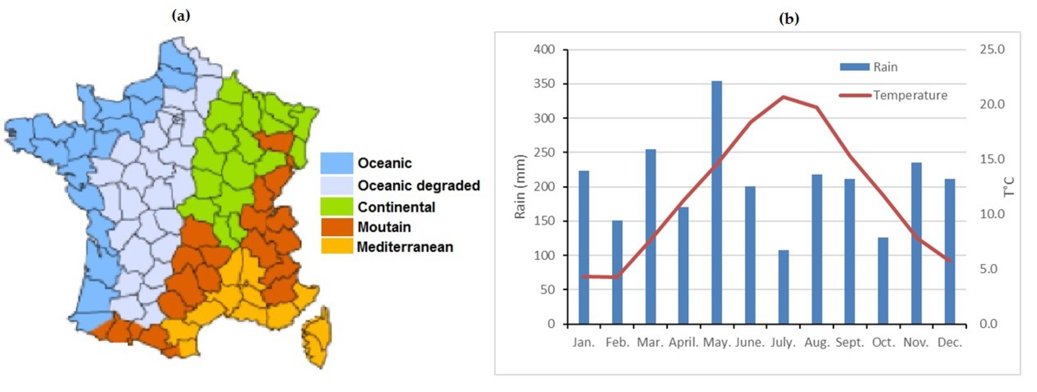
2.1. Experimental Site Description

The observation site and the monitoring procedure have been previously described by [39], as well as the occurrence of pollution events impacting the Saclay site [38]. Briefly, the observatory is located at Saclay, France (48.7247° N, 2.1488° E), 30 kilometers in the southwest of Paris. The observatory is known as the SIRTA station from the EU-ACTRIS network. The site is not under the direct influence of any chemical source, thus ideal for atmospheric gas, aerosol and bioaerosol observation. It is now referenced as an international intercomparison site for aerosol and bioaerosol instrumentation [42,43]. The sampling site is surrounded by crops, forest, and small residential villages, and can be impacted by strong winter and summer pollution events. Recently, this region has become more urbanized due the Paris-Saclay University building program, which is a part of the “Grand Paris” project; the subsequent drastic change in land use is expected to be modifying biogenic and anthropogenic emissions in the area.

2.2. Airborne Fungal Spores Monitoring Procedure

Airborne fungal spores (AFS) have been continuously monitored since July 2014 at Saclay, France. The observation period presented in this study runs from July 2014 to December, 2018 (234 weeks). Daily AFS concentrations were obtained with a volumetric impaction sampler (VIS), via a Hirst-type spore trap (VPPS 2000, Lanzoni, Bologna, Italy). The VPPS 2000 spore trap was located on the roof of the observatory at 15 m above the ground (152 m above sea level) without any neighboring vegetation. Under these conditions, the measurements obtained were expected to be representative of the regional sources. The air was continuously pumped through an orifice of 14 × 2 mm (28 mm²) always facing the prevailing winds at a flow rate of 10 L per minute. This instrument collected the impacted particles efficiently with an aerodynamic diameter between 2 μm and 200 μm on a rotating drum mounted with a 19 mm sticky tape (cellophane tape coated with silicone) [44]. The drum was changed weekly on the same day at the same time to minimize the sampling procedure errors. The counting and identification were performed by the French Monitoring Network of Aerobiology (Réseau National de Surveillance Aérobiologique, RNSA, Brussieu, France). Since RNSA belongs to the European Aeroallergen Network (EAN), it strictly follows the recommendations regarding the minimum requirements for the counting procedure. The standard analytical method used accounted for 10% of the surface area. Standard sampling, processing and analysis techniques have been well documented [45]. The quality assurance and the quality control of theses method were regularly made during the international intercomparison campaigns [46]. The daily concentrations obtained are expressed as concentrations of fungal spores per cubic meter of air. Analogous to pollen studies, the Main Spores Season (MSS) is defined as the duration time when fungal spores are present in the atmosphere in significant concentrations in a specific ecosystem. Therefore, it defines the main season start and end points. The MSS used in this study is the period during which the sum of daily mean fungal spore concentrations stands between 5% and 95% of the total sum. The terminology and the selection criteria used in this study follow the recommendation of [47].

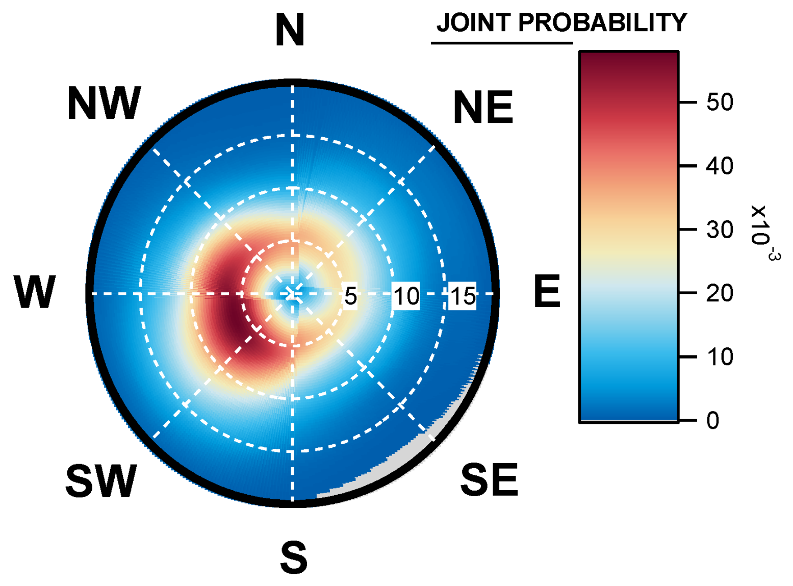
2.3. Investigation of the Geographical Origins of Airborne Fungal Spores

The investigation of the geographical origins of AFS was performed by coupling ambient concentrations with on-site measured wind data. At the Saclay observatory, meteorological parameters are provided by a weather station WXT520 (Vaisala, France). The measurements of wind speed (WS, m/s), wind direction (WD, Degrees), temperature (T, °C), relative humidity (RH, %), and cumulative rain (R, mm) are acquired every minute. A variant of two-dimension non-parametric wind regression (NWR) originally developed by [48], called the sustained wind incidence method (SWIM) developed by [49] has been used to identify the geographical origin of AFS. This variant takes into account the standard deviation of the wind speed and the wind direction on a daily basis.

Equation (1) below describes the calculation of SWIM,

$${\mathrm{S}}_{\mathrm{i}}=\frac{{\mathrm{C}}_{\mathrm{i}}·{\mathsf{{\rm Y}}}_{\mathrm{i}}}{\max \left({\mathrm{C}}_{\mathrm{i}}·{\mathsf{{\rm Y}}}_{\mathrm{i}}\right)}·\frac{\overline{\mathsf{\delta }}}{{\mathsf{\delta }}_{\mathrm{i}}}$$

(1)

where C_i, Υ_i, and δ represents respectively wind speed, wind direction, and wind direction standard deviation. This actually allows downwind daily concentration values associated with high atmospheric variability to be obtained during that day. Wind direction standard deviation was estimated by the 1-pass Yamartino equations [50]. This entire study was performed with ZeFir, a user-friendly tool for wind analysis [38]. More information can be found here: https://sites.google.com/site/ZeFirproject. This method was successfully applied for the first time to determine the geographical origin of pollen by [39].

2.4. Meteorological Aspects of the Saclay Ecosystem

France belongs to the temperate climate zone and four major climate types influence the territory regarding the climate over more than 30 years period [51]. The main one is in the west, mainly influenced by the ocean (Figure 1a, Oceanic, and Oceanic degraded). This climate is characterized by significant rainfall during autumn, winter and spring periods; less precipitation is observed during the summer period. Mean temperatures vary from 5 °C in winter to 21 °C in summer, as illustrated in Figure 1b. The Saclay observation site is dominated by an oceanic degraded climate (heavy rainfall during the dormancy period), relatively mild winter conditions with less than 47 days below 0 °C per year occurring between November to March and a relatively hot summer.

The Eastern region is characterized by a continental climate and the south of France exhibits a typical Mediterranean climate. The French mountains have their own climate characteristics, mainly driven by the altitude where temperatures are lower and precipitation higher on the slopes exposed to winds charged with humidity. A correct understanding of the ecosystem studied is necessary to grasp fungal spores purpose as their atmospheric concentration can be extremely variable [7].

2.5. Wind Prevalence at Saclay

Wind is an important factor for the dispersal and transport of (bio)aerosols far from their sources [35]. In order to better characterize the Saclay prevailing winds pattern between July 2014 and December 2018 the ZeFir source-receptor tool was used. The wind rose presented in Figure 2 indicate that air masses generally originate from west to south-west (oceanic), with speeds ranging between 5 to 12 km/h. A second wind regime is characterized by north (5°) to south-east (125°) winds, at speeds ranging from 2 to 7 km/h, bringing rather sunny skies, dry air and higher temperatures as reported by [39].

3. Results

In our study the complete identification of the fungal propagules at a genus level was not possible due to the used identification method (e.g 2.2). At this stage of our study no DNA or RNA analysis were done to complete the observations and particularly for Ascospores, Basidiospores and some optically unidentified spores. As it is the first time that these results are presented, they need to be compared with the literature to interpret the main parameters driving the AFS concentration in the Saclay ecosystem. This step is as a necessary prerequisite to use Zefir source receptor modeling tool to identify the geographical origin of airborne fungal spores impacting the observation site.

3.1. Interannuality of the Airborne Annual Fungal Spore Integral at Saclay

The interannuality of AFS Integral (AFSIn) was studied in depth. The annual sum of fungal spores ranges from 2.5 10⁶ Nb#/m³ to 5.2 10⁶ Nb#/m³. We observed a strong interannuality of the AFSIn and no biannual cycle has been found. Instead, a general decrease of the atmospheric concentration was found, as illustrated in Figure 3. The AFSIn data from January to June 2014 have been estimated by a linear modeling with the most basic model which is the simple linear regression where a variable X is explained and modeled by an affine function of a comparable variable Y. The interpolation of the Saclay data set from January to June 2014 has been done by comparing the daily concentrations of Paris and Saclay data set for year 2014 provided by the RNSA observations in Paris. The results obtained without the data set of the January to June 2014 were also showing a decrease of the atmospheric concentration (Figure A1, Appendix B) and pointed out the importance to follow the AFS all over the year as it is done at the Saclay observatory.

Such results are in accordance with those observed for total species records in Europe like reported by [52] with an AFSIn in 1989 of 2.10⁶ Nb#/m³. Similarly, in Greece, a general decrease in fungal spore levels in Thessaloniki was observed from 1987 to 2005 with a mean decrease of −52% compared to Saclay (−52%) [53]. The annual sum of fungal spores observed at Saclay is in the range of what has been observed in other oceanic environments in Europe, and is generally 3 to 4 times higher than in Mediterranean areas [54]. All the results obtained in these different ecosystems show a general decrease indicating that our observations are not linked to fluctuating changes.

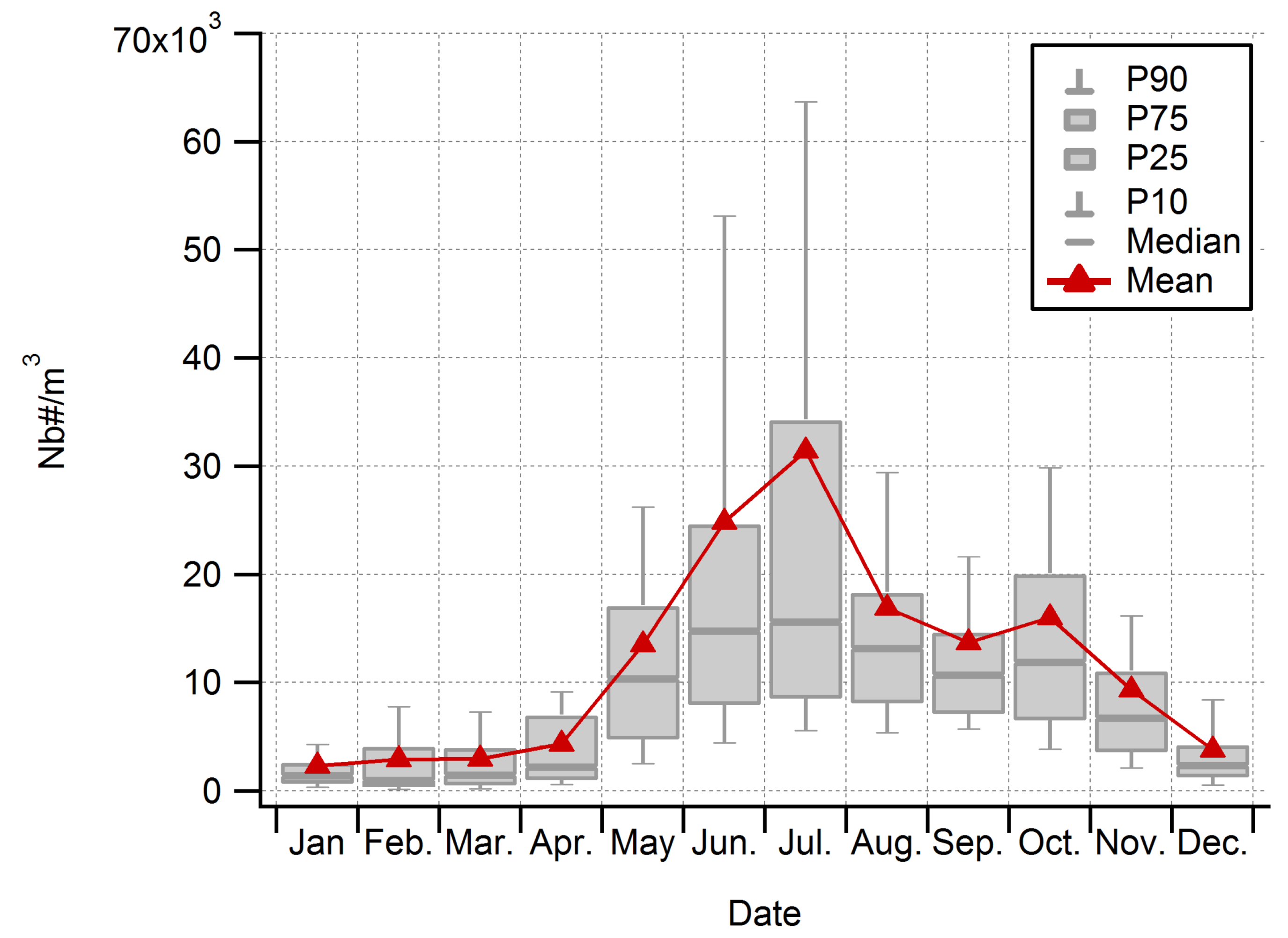
3.2. Seasonality of All Taxa Combined Concentrations at Saclay

The monthly mean distribution of all AFS concentrations averaged over the five years of measurements displays a clear bimodal seasonal cycle as illustrated in Figure 4. P90, P75, P25, and P10 represent the 90th, 75th, 25th, and 10th percentiles respectively. The monthly mean found for the MSS in the current study is found in May (11571 Nb#/m³) and ends in November (8472 Nb#/m³). The first maximum was observed in July (28,564 Nb#/m³) followed by a rapid decrease in September (12,456 Nb#/m³). A secondary maximum was noted in October (14,538.10³ Nb#/m³), followed by a sharp decrease in December (3439 Nb#/m³). Data are available in

Table A1. Values of monthly averages of fungal spores concentrations from January 2014 to December 2018.

2014–2018 (Nb#/m3)
Month	Mean	Max	Min
January	63,355	99,765	30,315
February	71,159	174,322	18,289
March	82,535	222,756	27,654
April	116,672	297,432	46,570
May	380,782	469,114	235,434
June	655,789	1,170,577	446,747
July	834,069	1,838,943	247,726
August	470,549	711,466	326,907
September	373,688	472,874	258,106
October	440,451	678,167	251,567
November	243,986	437,597	157,354
December	103,865	154,363	66,760

, Appendix A. In total, the fungal spore season is significant over 7 months in a year (from May to November), representing 58% of the year and 91% of the total AFS concentrations.

During the period of observation, no significantly high concentrations appear to drive up the statistical values that determine the two AFS seasonal peaks. 2014 and 2017 exhibit a clear seasonal cycle and the other years are more in a continuum from July to December as illustrated by Figure A2.

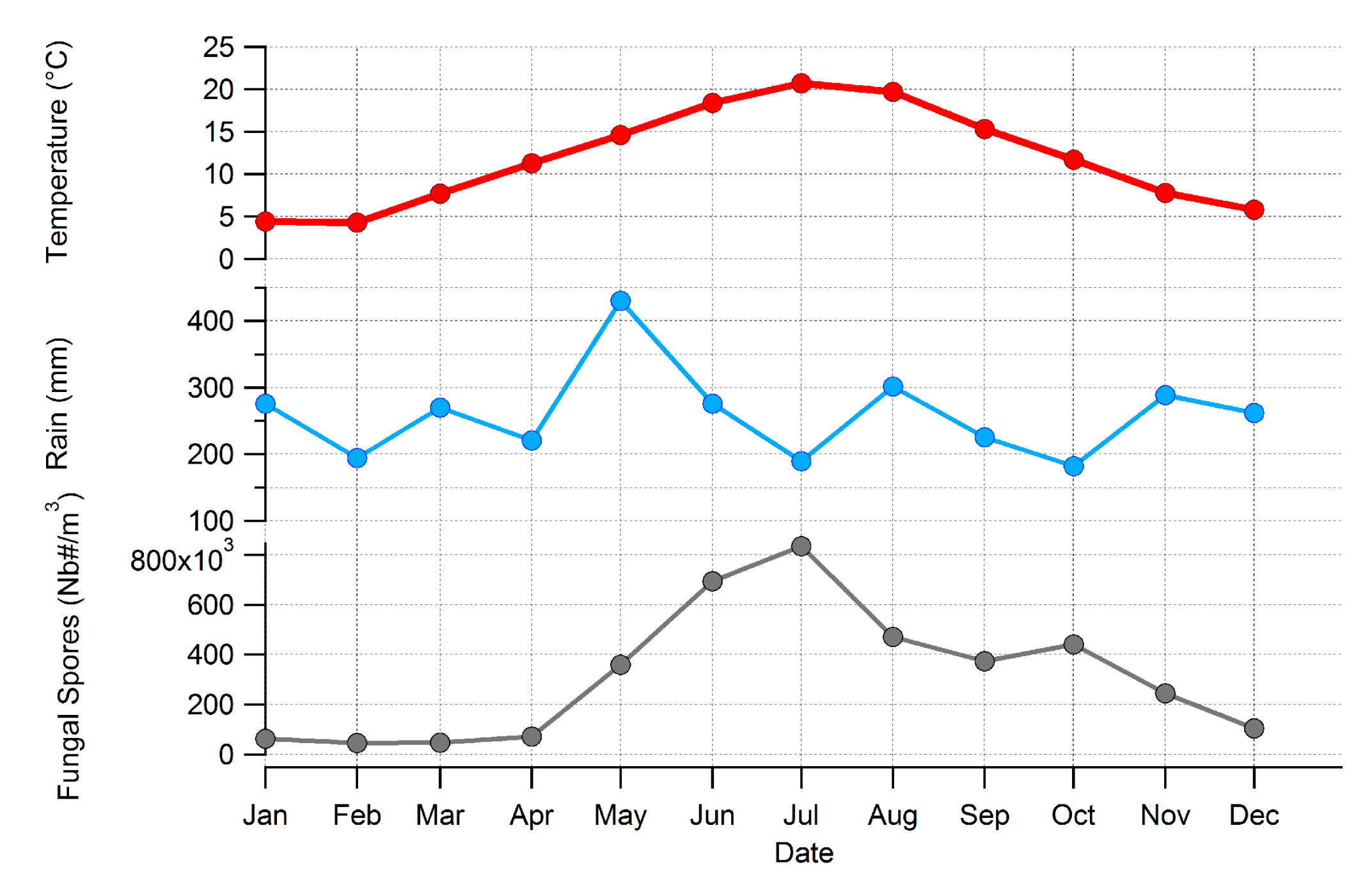
3.3. Major Parameters Driving the Seasonality of AFS Concentrations at Saclay

The observations made on the monthly means of temperature (°C), the monthly means of precipitation (mm) and the monthly mean concentrations of fungal spores, as illustrated in Figure 5, showed that the MSS starts when the mean temperature reaches an average value above 11 °C and not below (values are reported in Table A1 and

Table A2. Values of monthly averages temperature (°C) and relative humidity (RH%) for each year from 2014 to 2018.

2014–2018
Month	Mean AFS (Nb#/m3)	Mean T(°C)	Total Rain (mm)	Ratio (T/R)
January	63,355	4.4	276	0.0158
February	71,159	4.3	194	0.0220
March	82,535	7.7	270	0.0283
April	116,672	11.3	221	0.0511
May	380,782	14.6	430	0.0340
June	655,789	18.4	276	0.0668
July	834,069	20.7	189	0.1092
August	470,549	19.7	302	0.0655
September	373,688	15.3	233	0.0655
October	440,451	11.7	182	0.0643
November	243,986	7.8	289	0.0272
December	103,865	5.8	262	0.0220

). This result is important to understand how the production of fungal spores occurs: (1) the need for a certain amount of water; and (2) a mean temperature above 11 °C to start the growing process and the subsequent dispersal. Those observations are in full accordance with literature [6].

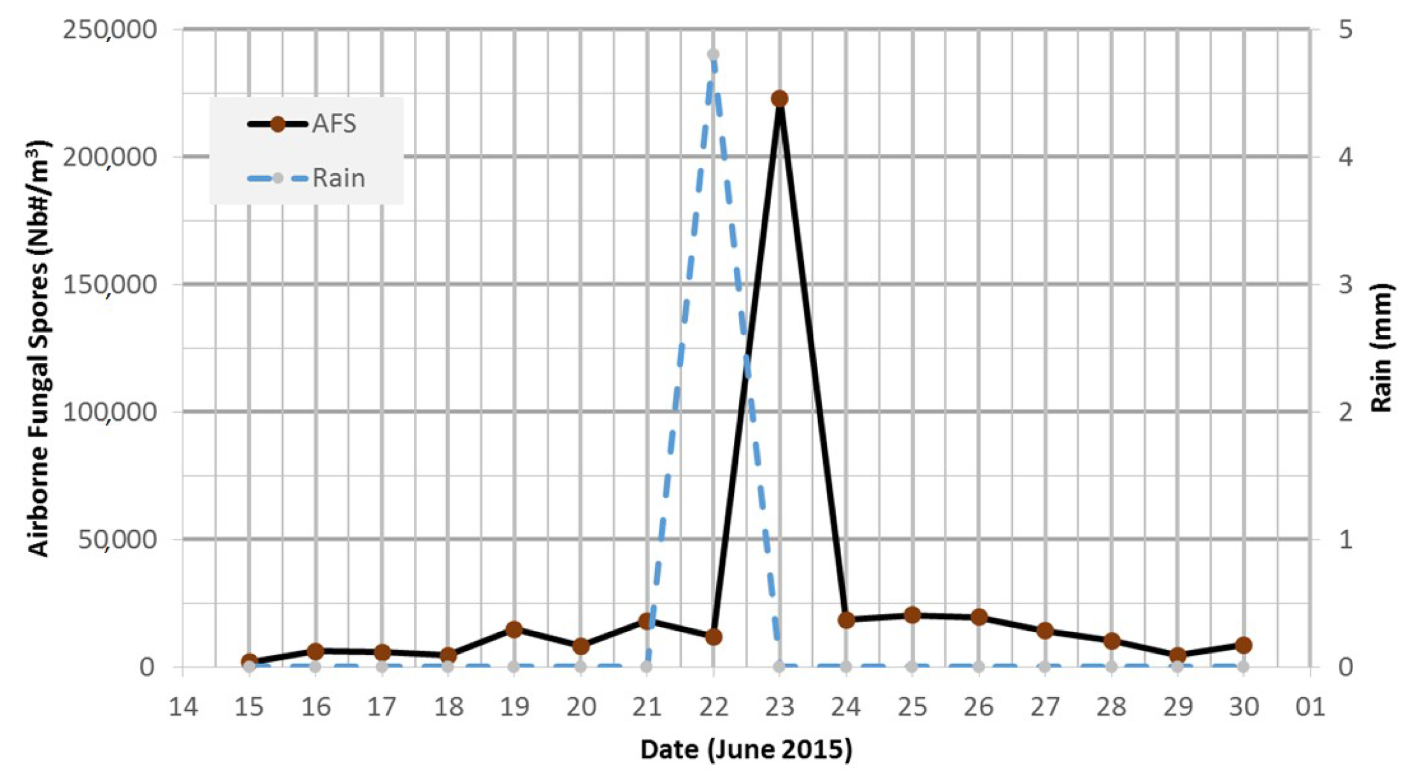
3.4. Main Spore Season and Daily Variability of Airborne Fungal Spore Concentrations at Saclay

The fungal propagule pattern at Saclay was found to be different from one year to the next likely due to the meteorological factors of variability (temperature, insolation, precipitation, atmospheric pollutants) as previously reported [55,56]. For each of the five years reported in the current study, the starts and the ends of the MSS are shown in

Table A3. Values of concentration in fungal spores and date of start and end season for each year from July 2014 to December 2018.

	2014	2015	2016	2017	2018
Total AFS (Nb#/m3)	5,395,236	2,982,527	4,038,344	4,351,542	2,465,766
5%	160	149,126	201,917	217,577	123,288
95%	4,500,000	2,833,401	3,836,427	4,133,965	2,342,478
Start Season	5 Apr	30 Apr	05 Apr	23 Mar	01 May
End Season	15 Nov	19 Nov	21 Nov	16 Nov	27 Dec

. The calculation applied was the same as what has been previously employed [57].

As shown in Figure 6, the fungal spore concentrations can be extremely variable both in time and intensity. As an example, a high concentration’s episode occurred in June 2015 as the weather conditions were remarkably hot and dry for the season. Hence an increase in the AFS concentrations from 10 × 10³ Nb#/m³ on 22 June rising to 256 × 10³ Nb#/m³ on 23 June and decreasing back to 10 × 10³ Nb#/m³ on 24 June was noted. This exceptional episode has been characterized using several on-line techniques to understand the processes involved in creating the bloom of bioaerosols that can occur in water-stressed environments [58]. It turned out that during 2015 the temperature in the region of Saclay was greater by 1.5% from annual seasonal normal temperatures with the month of June being particularly hotter and dryer (+5%) than “normal” records. On 23 June a precipitation event occurred, and, at the end of the rain episode, the concentration of total fungal spores got multiplied by a factor 25. This observation is consistent with other studies showing that air temperature is the main physical parameter driving AFS concentrations but is not effective without the presence of water and most typically, a rain shower which increase the bioaerosol concentrations after several hours [59,60].

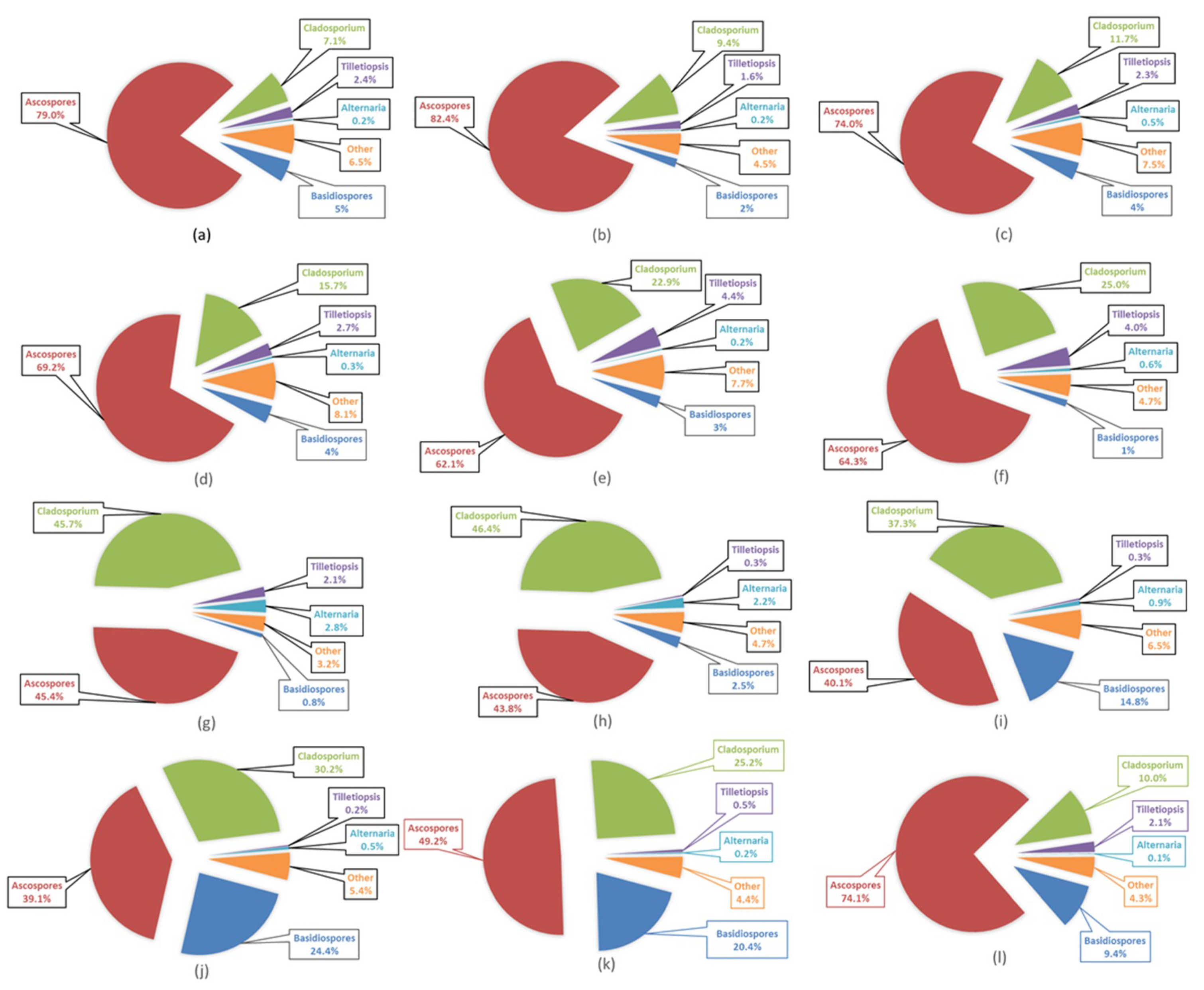
3.5. Airborne Fungal Spore Characteristics at Saclay

To date, the classification regarding the phylum is still under progress due to novel technics of identifications [61]. In our study, 30 types of propagules were identified and classified under the Universal Biological Indexer and Organizer (uBio) [62]. The results are reported in

Table A4. Physical characteristics of the 30 propagules types identified at Saclay (A = Ascospore, B = Basidiospore, C = Conidia, M = Myxomycetes, S = Sporangiospore, T = Teliospore, U = Urediniospore) adapted from the Universal Biological Indexer and Organizer, [61].

Name	Phylum	Spore Type	Optical Spore Size (μm)	Habitat
Alternaria	Ascomycota	C	20–80	Soil, plants, and vegetables, mainly develop on decaying plants, especially cereals and hay.
Ascospores	Ascomycota	A	15–40	All the sexually produced fungal spores formed within an ascus.
Aspergillaceae	Ascomycota	A	2–10	Everywhere in nature (e.g., soil, decaying organic debris, and compost), in grains storage areas.
Basidiospores	Basidiomycota	B	5–15	Mainly in forests and woodlands, especially in the autumn.
Botrytis	Ascomycota	C	5–10	Ubiquitous, polyphagous, and necrotrophic, also abundant in soil.
Cercospora	Ascomycota	C	2–5 × 50–325	Leaf parasites of chard, sugar beet, carrot, lettuce, and maize.
Chaetomium	Ascomycota	A	10	On plant debris, soil, straw, and dung, also on wooden products.
Cladosporium	Ascomycota	C	4–11	Saprophyte, on soil, plants, and cereals, colonizes very varied substrates (foodstuff, paper, textile, etc.).
Didymella	Ascomycota	A	3–15 × 1–4	On the leaves of barley and wheat, berries and vegetable cultivation (e.g., peas, tomatoes, gherkins, and cucumbers).
Entomophthora	Zygomycota	C	11–18 × 8–15	On flies, causes a fatal disease.
Epicoccum	Ascomycota	C	20	On soil and senescent, dying or dead plants, especially cereals, beans, potatoes, peas, and peaches.
Erysiphe	Ascomycota	C	30–60	On plants, pathogens which cause powdery mildew.
Fusarium	Ascomycota	C	25–68 × 3–6	Mainly in cereal crops (grains, straw, and hay), also invade fresh fruits and vegetables.
Fusicladium	Ascomycota	A		On plants, and most are pathogens.
Ganoderma	Basidiomycota	B	6–10	At the base and on stumps of deciduous trees, (oak, beech, and poplar), also on the roots of some fruit trees.
Helicomyces	Ascomycota	A and C	70–140 × 2–3 and 14–21	Most are aquatic, on marsh plants, on dead leaves, on grass stems, or on shelled wood.
Helminthosporium	Ascomycota	C	40–118 × 11–20	In humid areas, on grasses (above all barley and corn), also on dead branches and fallen branches of most trees and shrubs.
Myxomycetes	Mycetozoa	M	5–24	In open forests, on deadwood, the bark of living trees, rotting plant material, soil and animal excrements.
Nigrospora	Ascomycota	C	13–15 × 10–13, 18–21 × 14–15, 18–24	In air, soil, various decaying plants, and some cereal grains; it is rarely found growing indoors.
Peronospora	Chromista	S	15–35	Plant pathogens of herbaceous dicotyledonous plants, (mildew).
Pithomyces	Ascomycota	C	15–25	Ubiquitous on soil, also on dead leaves and fodder grasses, occasionally in indoor environment.
Pleospora	Ascomycota	A	30–33 × 14–15	A plant pathogen with a cosmopolitan distribution, infecting all kinds of herbaceous debris and crops.
Polythrincium	Ascomycota	C	5 × 1.5	On leaves, especially on leaves of red clover
Sporobolomyces	Basidiomycota	C	5–25	Yeast in air, on humans, mammals, birds, the environment, and plants.
Stemphylium	Ascomycota	C	22–35	In the agricultural environment, on dead tissues, animal or plant fibers (straw), also parasitic plants.
Tilletiopsis	Basidiomycota	T	1–3	Parasites of flowering plants.
Torula	Ascomycota	C	3–4	Yeast, on stems of dead herbaceous plants and on the leaves of barley and mature wheat.
Trichothecium	Ascomycota	C	8–10 × 12–18	Cosmopolitan, in various habitats ranging from leaf litter to fruit crops.
Uredospores	Basidiomycota	U	15–25	Parasite of many plant families, cereals are the most common hosts.
Ustilago	Basidiomycota	T	5–10	Parasite of herbs (Poaceae), mainly cereals (maize and teosinte).

. During the period of observation, i.e., from July 2014 to December 2018, the relative proportion of the Ascomycota (AMC) and Basidiomycota (BMC) at a phylum level were calculated without DNA or RNA analysis in our atmospheric samples. The results were compared with the methodology proposed by [15] regarding the fungal diversity over land and oceans to determine a biogeography in the air. The ratio BMC/AMC in our ecosystem is dominated by AMC (Figure 7). This is consistent with the predominance of BMC and AMC in the biosphere, where they account for 98% of the known species and also with the Oceanic Degraded climate characteristics of the Saclay site, in reference to marine sites as reported by [63].

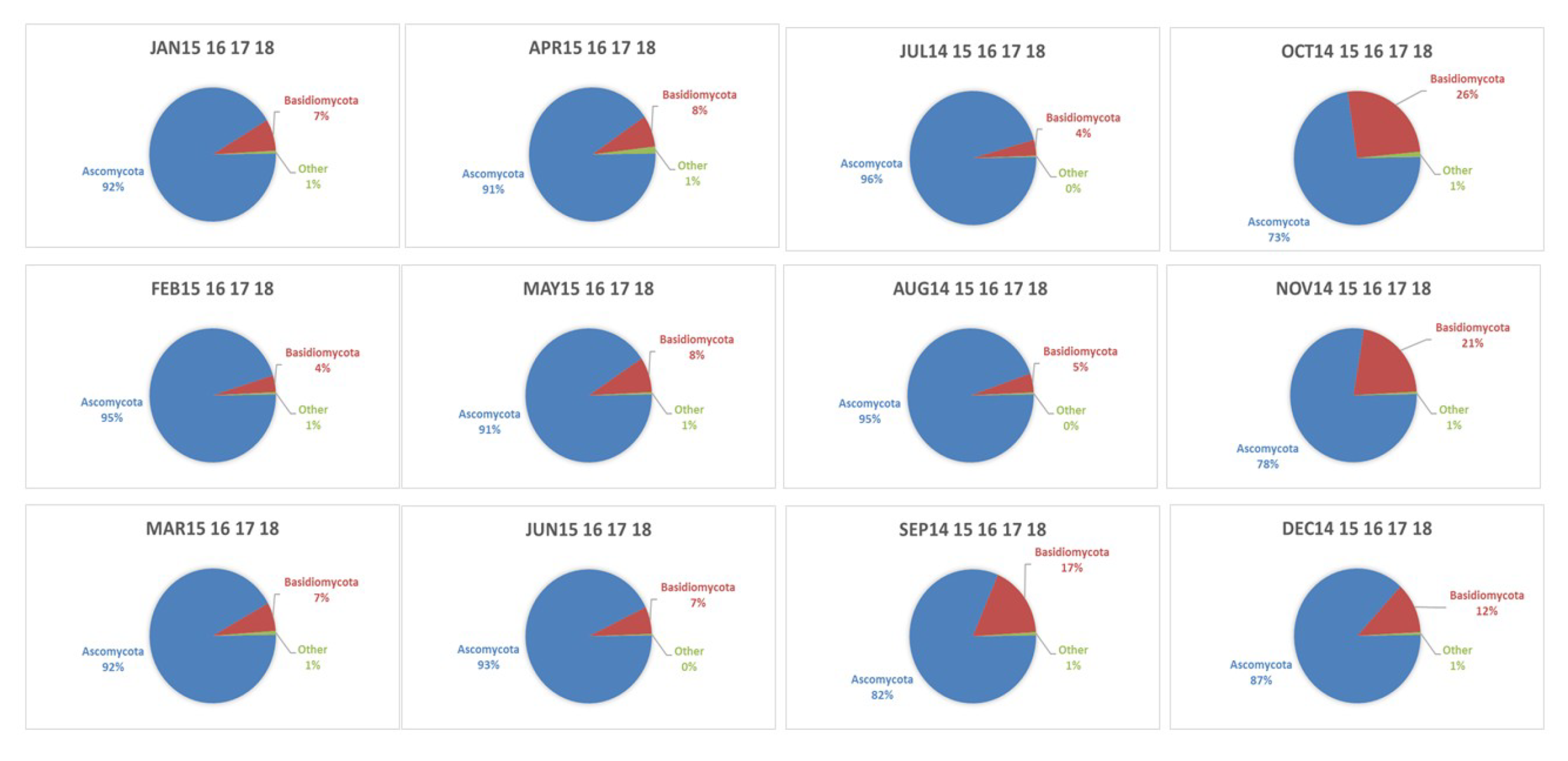
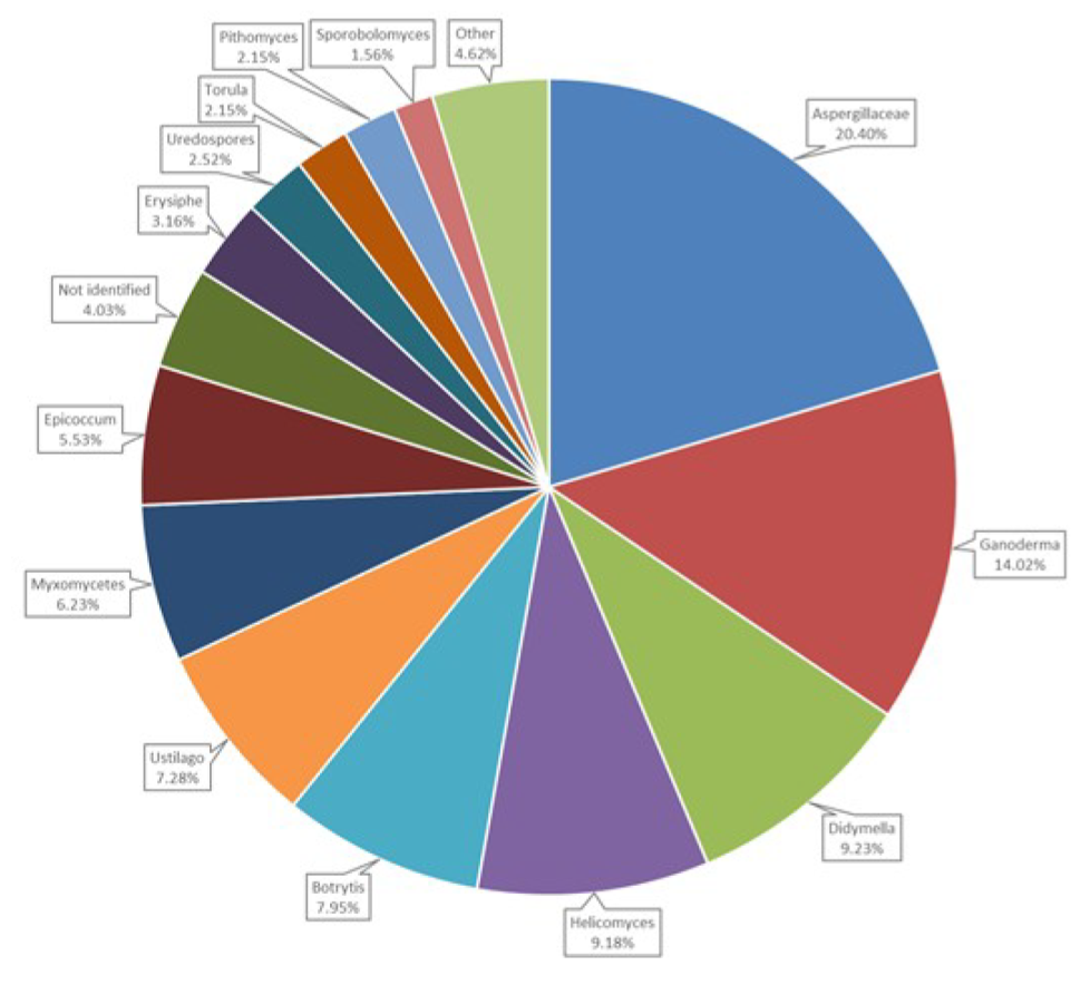
3.6. Airborne Fungal Spore Diversity at Saclay

The mean concentrations and percentages of the 30 atmospheric fungal propagules found at Saclay are reported in

Table A5. Mean concentrations and percentages of the 30 fungal propagules identified through a light microscope at Saclay from July 2014 to December 2018.

	2014–2018		2014		2015		2016		2017		2018
	Avg (Nb#/m3)	(%)	Avg (Nb#/m3)	(%)	Avg (Nb#/m3)	(%)	Avg (Nb#/m3)	(%)	Avg (Nb#/m3)	(%)	Avg (Nb#/m3)	(%)
Alternaria	257	2.377	277	1.386	63	0.746	106	0.958	202	1.696	115	1.604
Ascospores	5568	51.548	11,560	57.881	3418	40.519	6888	62.082	5784	48.474	2686	37.407
Aspergillaceae	181	1.679	124	0.620	87	1.031	104	0.942	145	1.217	88	1.222
Unidentified	118	1.097	51	0.254	36	0.422	21	0.190	12	0.098	3	0.046
Basidiospores	960	8.887	1284	6.427	1099	13.030	449	4.049	1243	10.413	213	2.969
Botrytis	109	1.011	56	0.282	17	0.200	98	0.885	27	0.227	20	0.284
Cercospora	52	0.480	6	0.030	6	0.069	11	0.099	11	0.090	6	0.081
Chaetomium	33	0.306	0	0.001	1	0.012	1	0.006	0	0.003	1	0.016
Cladosporium	3731	34.544	5795	29.015	3289	38.989	2784	25.089	3888	32.585	3644	50.744
Didymella	190	1.760	4	0.022	31	0.364	56	0.501	89	0.744	47	0.657
Entomophthora	52	0.481	0	0.000	0	0.000	0	0.003	0	0.000	0	0.000
Epicoccum	80	0.743	77	0.384	26	0.305	24	0.217	28	0.238	17	0.239
Erysiphe	65	0.602	19	0.096	26	0.302	22	0.199	10	0.085	9	0.130
Fusarium	36	0.337	0	0.001	3	0.034	2	0.019	1	0.012	0	0.002
Fusicladium	34	0.314	3	0.017	4	0.045	1	0.010	2	0.018	2	0.025
Ganoderma	131	1.212	141	0.704	65	0.772	64	0.575	74	0.619	68	0.948
Helicomyces	225	2.084	15	0.077	38	0.453	58	0.523	61	0.510	60	0.837
Helminthosporium	32	0.297	1	0.007	1	0.010	0	0.002	1	0.008	0	0.006
Myxomycetes	92	0.854	44	0.220	19	0.220	28	0.252	40	0.334	44	0.609
Nigrospora	29	0.266	1	0.007	1	0.016	0	0.001	1	0.006	0	0.006
Peronospora	45	0.420	16	0.078	2	0.021	2	0.017	5	0.040	2	0.022
Pithomyces	136	1.260	21	0.103	5	0.055	12	0.107	11	0.095	15	0.203
Pleospora	52	0.481	0	0.000	0	0.004	0	0.002	0	0.000	0	0.000
Polythrincium	40	0.373	22	0.109	3	0.030	3	0.029	6	0.048	2	0.026
Sporobolomyces	160	1.477	43	0.218	15	0.179	0	0.000	0	0.001	0	0.000
Stemphylium	29	0.272	2	0.010	1	0.008	1	0.007	1	0.010	0	0.006
Tilletiopsis	393	3.640	291	1.457	103	1.221	306	2.758	231	1.932	98	1.360
Torula	49	0.456	23	0.115	9	0.112	12	0.105	12	0.103	7	0.101
Trichothecium	49	0.453	1	0.004	0	0.000	1	0.007	0	0.001	0	0.000
Uredospores	64	0.595	44	0.221	8	0.093	15	0.133	8	0.069	8	0.109
Ustilago	120	1.109	51	0.256	62	0.737	26	0.234	39	0.324	25	0.343

. To better understand the variability of AFS at Saclay and the relative proportion of allergenic fungal spores, we analyzed the major classes of fungal spore propagules present in the air. Figure 8 displays the obtained pattern which takes into account 95% of the total AFS. AMC contributes to 85% of the total AFS, driven by Ascopores (51%), Cladosporium (33%), and Alternaria (1%), while BMC only represents 10% of AFSIn through the contribution of the Basidiospores (8%) and Tilletiopsis (2%) taxa. Their seasonality was investigated (Figure A3, Appendix B) but the time variable does not appear to determine the predominance of AMC in the Saclay environment, which therefore calls for screening the air mass origins.

As illustrated in Figure 8, the known allergenic taxa monitored at Saclay, which are Cladosporium and Alternaria, represent 34% of the AFSIn and in the AMC phylum. Clearly, there is a major reservoir for allergenic species but, at this stage of development, only genotyping analysis could reveal what are the species to be found in the Ascospores and Basidiospores reservoir.

4. Discussion

The interannual, seasonal and daily variability of total and specific AFSIn concentrations at Saclay are discussed and compared to the literature. The geographical origins of the main AFS impacting the observation site were thus assessed and discussed through the use of the Zefir source-receptor model. For the purpose of investigating the origins and point sources of AFS impacting Saclay will be also discussed

4.1. Factors Controling the Airborne Fungal Spore Concentrations

In the ecosystem of Saclay, water is not a limiting factor, which makes air temperature the only driver of the AFS seasonality, as illustrated by Figure A4 and Figure A5. This result is in accordance with recent findings from [55]. In an attempt to model the seasonal cycle of AFS at Saclay, we explored different calculation procedures based on our understanding of the impact of rainfall on AFS concentrations. We found that by normalizing the monthly mean temperature by the monthly mean precipitation, we could reasonably reproduce the seasonal cycle of AFS at Saclay (Figure 9) and values reported in Table A2.

In the literature, rain has often been cited as the most efficient agent for the wet removal of bioaerosols [64]. However, precipitation alone would possibly be a poor driving parameter on regression models [35] for two main reasons 1) the annual variation of daily precipitation values does not closely correlate with the concentrations measured during dry or wet conditions, (2) precipitation on a daily basis presents high variability in time and space (rain patches). Therefore, instead of considering precipitation data, some works suggested to follow rain showers as a favorable trigger of PBAP generation [59]. The second BIOaerosol DETECTion campaign in 2015 (BIODETECT 2015) in Saclay provides an interesting illustration of the triggering property of rain showers on PBAPs. As described in Section 3.6, June in 2015 was particularly hot and dry. The AFS concentrations were low for the season compared to 2016 and 2017. A moderate rainfall event occurred on 23 June 2015 providing 4.8 mm of water in four hours (e.g., 1 mm measured is equivalent to 1 L/m²). Despite this relatively low amount of water, right after the shower, the concentrations in AFS have been multiplied by 25 from 12,000 Nb#/m³ to 226,056 Nb#/m³, then went back to 14,000 Nb#/m³ the day after as reported in (

Table A6. Daily concentrations (Nb#/m3) of the five principal propagules during the episode of June 2015.

	Alternaria	Ascospores	Basidiospores	Cladosporium	Tilletiopsis
17/06/2015	0	746	52	3907	26
18/06/2015	0	1311	78	2313	257
19/06/2015	78	6194	0	5989	1106
20/06/2015	78	1157	103	5166	155
21/06/2015	103	6888	180	7068	2699
22/06/2015	26	5397	257	5269	206
23/06/2015	0	205,755	78	13,133	1799
24/06/2015	0	1208	155	16,037	309
25/06/2015	78	1311	129	18,068	52
26/06/2015	257	1028	52	16,962	0
27/06/2015	52	360	26	13,005	0

) and illustrated by Figure 10. This event can be typically defined as a “splash dispersal” [65]. These spores are known to be hydrofugal and can be easily dispersed by the impact of raindrops [66]. But more interesting is the proportion of the different species. As expected, Ascospores were dominant; Cladosporium and Alternaria were not affected but Ustilago, Dydimella, and Helicomyces concentrations increased from 0 to 1131 Nb#/m³, 103 to 232 Nb#/m³, and 0 to 283 Nb#/m³, respectively. Ustilago is known to be a cereal and herb pathogen (Table A2) and the strong increase observed coincided with the end of the Poaceae pollen season, as reported by [39]. In this specific period, Poaceae was in early decline due to the very hot climate conditions. The rain shower suddenly favored the release of these fungi which was living and growing in this type of habitat. We also observed that the concentrations of Cladosporium increased slowly to reach a maximum 2 days after. This is consistent with the study of [67] on the growing processes.

Pathogenic AFS are a key concern which requires a better understanding of their control factors as they need a host (plants or animals) for their own development. For lower case, Entomophthora species, a lethal fungal parasite affecting a type of fly, the Musca domestica [41] was observed for the first time in May 2016 at Saclay, in relatively high concentrations. The presence of this fungal parasite has been explained by the entomologist Sandrine Provots (personal communication) by the late produce egg hatching and larval formation. Indeed, the late start of the spring due to cold weather [65] created a delay in the fly reproductions at a regional scale. Consequently, an explosion of flies occurs and, a remarkable proliferation of this pathogen in the early days of May as reported by the French National Survey of Crops contamination [66]. This episode has generated a drastic increase of the atmospheric concentrations of Entomophthora’s fungal spores and they were transported and detected at Saclay far from the point source. It pointed out one more time the indirect role of the local and regional meteorology in the exhalation or inhibition of AFS and particularly the dispersion of specific AFS pathogens with unknown pathogenicity consequences on human and animals. The variability of fungal spore concentrations is therefore strongly dependent on the related ecosystem and on its local and regional meteorological characteristics. In particular, some species undergo strong differences in growth following wet, dry, or “splash” discharges. These processes of discharge can subsequently affect the concentrations of the chemical tracers in the PM10 fraction. Moreover, to better understand the effects of rainfall events on fungal spore diversity, abundance and dispersal processes, models need to integrate rain and temperature as well as dew point data at the finest resolution possible.

4.2. Interannuality and Global Increase of Specific AFSIn Concentrations

The total concentrations of AFS are in general analyzed in the literature in a context of global warming and for allergenic purposes [12,53,67]. It is admitted today that fungal spores are very sensitive to temperature and water (e.g., relative humidity and rain for their proper development [15]. It is the case on Earth but also in confined and much stressed environments like the International Space Station [68].

On a year-to-year basis, the results of our 5-year study display strong variations in the interannuality of the five main fungal taxa spores identified (Figure 11). We also analyze Ustilago as it is a strong plant pathogen on culture [36] and present on the strong allergenic Poaceae pollen

We investigated the influence of the meteorological conditions that then occurred in France. During our period of observation indeed, 2015 and 2018 where hot and dry. In more details, 2015 was characterized by a deviation of +1.5 °C compared to the seasonal normal and a loss close to 20% in the total precipitations all over the country. The year 2018 was the hottest since 1959 in France with a measured anomaly of +1.4 °C (+2 °C in the continental part alone) and was relatively dry all over France (global loss in precipitation of 10%). In the north half of the country, including Saclay, a loss of more than 20% in the total rain water was observed [69]. In contrast, 2014 was the second hottest year after 2018 but benefited in the northern half of France from an additional 20% of precipitations. The years 2016 and 2017 stood in the normal seasonal range (temperature and rain), but 2017 was hot and humid in the northern part of France and quite close to what it has been observed for 2014.

The general decrease of the concentration observed in the AFSIn was mainly due to the predominance of Ascospores in the Saclay ecosystem. Cladosporium shows moderate biannual cycle compared to the other taxa studied. Ustilago and Basidiospores presented similar patterns: (1) a strong biannual cycle and (2) strong sensitivity to hot temperature while Tilletiopsis concentrations are strongly affected by hot weather. Interestingly, given they are all BMC and that continental climate is expected to be hotter, our observations suggest one hypothesis of the enrichment in the ratio BMC/AMC in continental ecosystem. The effect of the D_a of the fungal propagules as proposed by [15] is perhaps not the only factor controlling the ratio BMC/AMC and could change in the future. Moreover, the growing kinetics is strongly dependent on temperature as reported by [70]. To understand the differences between the annual variability of the different taxa, we investigated the impact in the cycle of the land use in “Big Cultures” which include wheat, maize, ragweed, onions, and tomatoes [71]. We did not find any correlation in the annual cycles, but evidenced a probable link with the general increasing trend in the total agricultural production for humans. This last point supports idea that the presence of agricultural fields is not a limiting factor for the emission of AFS in the air, unlike rain and temperature. These differences from-to-year can explain the differences observed in the individual ratio of BMC and AMC as illustrated by the Figure A3.

Preliminary conclusions point out, as expected, that all taxa do not have the same response to an elevation of temperature and rainfalls—in particular, Ascospores and Tilletiopsis seem to be very sensitive to temperature and hydrological stress. It is noticeable that, since 1990, temperature in France has always stood between +0.5 and +1.4°C, up +2 °C in some specific regions, over the normal annual mean computed from 1981 to 2010, as reported in [69]. Consequently, our 5-year study displays a strong interannuality of the monitored taxa. Cladosporium, Ustilago, and Basidiospores are characterized by a bi-annual cycle in accordance with that previously reported [53,67]. The general decrease observed in the total AFS is mainly due to the predominance of Ascospores followed by Basidiospores.

4.3. Seasonality of BMC and AMC

Continuous measurements of AFS are important to increase the knowledge as the seasonality can be different in time and in variability as illustrated by Figure A6. In the study, as Saclay is not referenced as a marine or coastal site, it was expected a higher abundance for BMC. One explanation for this observation can be found in the size properties of AFS. BMC are expected to have shorter atmospheric residence times, therefore are unsuitable to undergo long-range transport. The BMC/AMC ratio is thus expected to decrease with increasing distance from the sea. As Saclay is 250 km from the ocean and impacted by marine air masses it would mean that the distance effect would need to be greater than 250 km in order to see a difference in the BMC/AMC ratio as reported by [15]. During our five-year observation period, we noticed that the ratio of BMC/AMC was changing during the season (Figure 12). This result does not affect the global ratio of BMC/AMC (e.g., Figure 7) but points out (1) the importance to consider BMC/AMC ratios by season for one given ecosystem and (2) to have a better understanding of the BMC/AMC ratio as a function of environmental considerations as proposed by [15]. In 2017, [72] showed similar and finer results regarding the seasonality of BMC/AMC using DNA analysis in several northern Europe locations and the observations suggested that the biodiversity of fungal spores can be observed after 900 km from an ecosystem to another one with consequences on the variation in the BMC/AMC ratios.

In the literature it has been found that emissions of fungal spores from the oceans (10 Mg per year) are several orders of magnitude smaller than from inland surfaces (30–50 Tg per year) [18,19]. Emissions are characterized by specific BMC/AMC ratios: high ratios of BMC/AMC in marine or coastal sites and low ratios of BMC/AMC in continental sites [15]. The phyla richness of BMC has been explained regarding the size of the AFS. BMC are considered to be 5 to 10 μm (D_a) in size and AMC to be between 2 and 5 μm (D_a). BMC is enhanced in the coarse fraction (>2.5 μm), whereas the taxa richness of AMC is enhanced in the fine fraction (<2.5 μm) of continental air particulate matter due to their shorter atmospheric residence times. Our observation suggests that additional processes are involved in relation with temperature, rainfall and the ecosystem characteristics, in particular land use. As continental areas present higher temperature levels during spring and summer than marine areas, Ascospores or Basidiospores proliferation can be inhibited. In the same time, cereal and herbs are largely present in continental regions which possibly increase the presence of BMC spores like Ustilago and other Basidiospores. As described by [54] in the region of Madrid (hot and dry summer), during the MSS, AMC were not predominating due to hot and dry weather. Another preliminary conclusion suggests that the size of the spores is not the only factor that can explain the variation in the ratio of BMC/AMC. Other drivers could be (1) the climate of the ecosystem studied by determining the proportion of the main phyla and also the proportion in species in the same phyla and (2) the land use related to the culture of cereals or the presence of herbs—France among the European countries has the largest crops mainly located in the North and in its continental part (e.g., Figure 1) followed by Germany [73]. This aspect should be taken into account in the future in a context of global warming regarding the potential formation of GCCN, CCN, and IN [9,74].

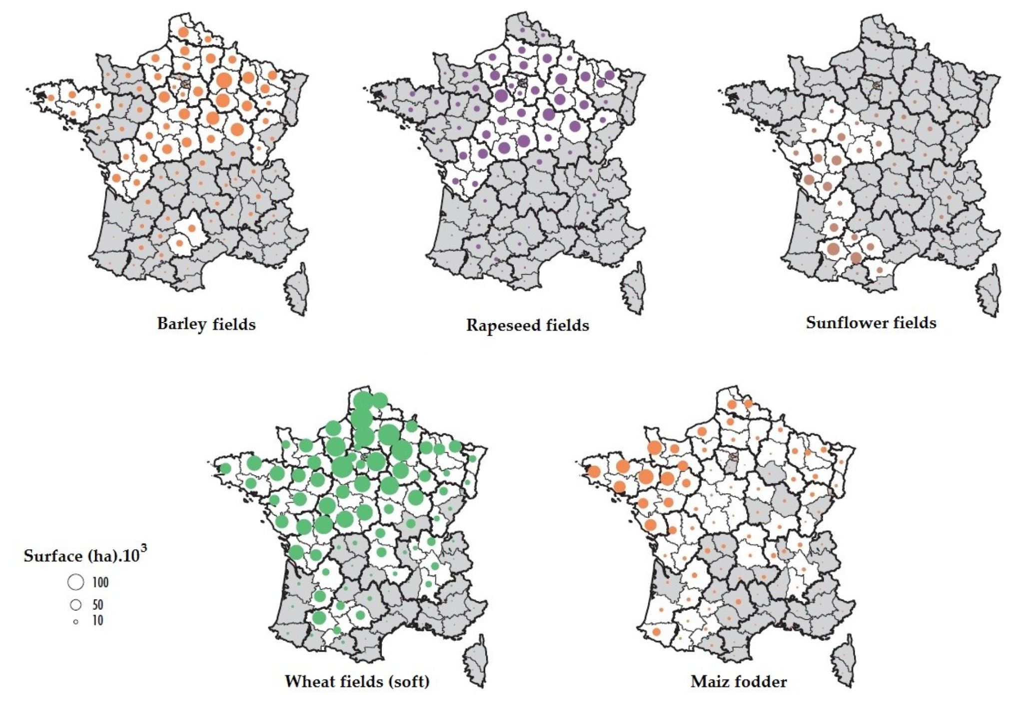
4.4. Geographical Origins of AFS Impacting the Observation Site

The calculations using ZeFir from this 5-year dataset showed an interesting result regarding the general origin of AFS concentrations. The model designates a main origin from the northwest sector, that is, independent from the SW prevailing winds (Figure 2), however still in the general “wet” W sector, which mostly carries marine air masses. Two point-sources were identified, the major one is associated with wind speeds ranging from 10 km/h to 13 km/h and a minor one with wind speeds of 17 km/h (Figure 13). We also evaluate the geographical origin of total AFS by running the model year to year as illustrated by Figure A7 to investigate the effect of the meteorology on the Saclay ecosystem.

Figure 14 reveals that Saclay is impacted by both local and regional sources. Among the main fungal spores (95% of the species present in the air Section 2.2) Ascospores and Basiodospores which are both wet spores are clearly originating from different areas: North West for Ascospores (marine/costal area) and North East for Basiodospores (continental area). Cladosporium and Tilletiopsis were clearly originating from the NW sector. For Alternaria, the results pointed out a regional origin, possibly related to large agricultural parcels of rapeseed and sun flower (Figure A8) as Alternaria is known to be a plant pathogen of those crops [73,75].

4.5. Case of Studies: The Geographical Origins of Plant or Human Pathogens

To go further in our understanding on the geographical origin of specific AFS we ran the model for eight species representing 65 % on the remaining 5% of the AFS (Figure A9), thus less abundant but determining as most of them being referenced as human or plant pathogens. The result obtained for Aspergillaceae, Ganoderma, Myxomycetes and Ustilago depicts a clear North to North East origin as illustrated by Figure 15. Aspergillaceae and Myxomycetes are two taxa known to grow in open forest on decaying material (Table A4), while the habitat of Ustilago is known to be Poaceae and cereals, as already mentioned. This happens to be in close agreement with our results on the geographical origin of Betulaceae and Poaceae pollen grains impacting Saclay [39].

We also run the model for Didymella, Helicomyces, Botryris, and Entomophthora, which ended to originate from the NW and the SSW sectors (Figure 16). As reported in Table A3, Didymella and Helicomyces can grow on barley and corn leaves. By comparing the geographical origin computed by the model and the map of barley and corn fields in France (Figure A9) we observed that the model accounted for the sources of these two fungi. In particular, Helicomyces originated from SSW brought by strong winds ranging from 15 to 20 kmh. This result is of importance for the optimization of the Zefir model to localize more precisely specific point sources by comparing the distance of the source and the spots founded by the model as a function of wind speed in km/h. Botrytris is polyphagous and the main point source was identified on the NW sector. We attempted to identify the geographical origin of Entomophthora and we found a regional origin in the NW sector. We also observed the limits of the model when the data set used to find the origin and point sources is too limited (only two days in 2016).

The use of pesticides on large agricultural parcels can inhibit the production of AFS by the crops but have no significant disturbance on production from forests or prairies, allowing the natural growth of specific pathogens. The hypothesis regarding the use of chemicals as a control factor of the proliferation of fungi on crops needs to be investigated in more details in future works, since our work suggests a same point source for Ustilago and Poaceae pollen. This last point must be taken in account for cross contamination in land in rotating land use [76].

5. Conclusions

The objectives of this work were, firstly, to understand the atmospheric variability of the main airborne fungal spores (AFS) present at Saclay, a suburban area of Paris and, secondly, to apply a source receptor model to attempt identifying their geographical origin. Several case studies served to investigate the link between land uses and production of AFS. In the Saclay oceanic degraded ecosystem, 30 fungal airborne spore taxa were identified following palynological methods. In relation with the classification used in this work, Ascomycota (AMC) were predominant (89%) followed by Basidiomycota (BMC, 10%). Ascospores were the main taxa (51%), then Cladosporium (33%), Basidiospores (8%), Tilletiopsis (2%), and Alternaria (1%). We observed a strong interannuality and a general decrease in the total AFSi concentrations over our 5-year study, mainly driven by the “wet spores” Ascospores and Basidiospores, while the “dry spores” Cladosporium and Alternaria had increasing trends. The year-to-year variability resulted from hot/cold temperature combined to dry/wet conditions. The AFS concentrations showed a clear bimodal seasonal cycle and the main spores season (MSS) is strongly affected by meteorological factors like temperature and rainfall. A mean of 11 °C has been found to allow the start of the season and the first maximum occurs in July (32,000 Nb#/m³) while the second occurs in October (17,000 Nb#/m³) as illustrated in Figure 4. The BMC/AMC also showed a seasonality suggesting that the size of the spores is not the only factor that can explain the variation in the BMC/AMC ratio. Preliminary results pointed out that fungal propagules do not have the same response to an elevation of temperature or can be very sensitive to temperature and hydrological stress. We also pointed out that they do not have the same geographical origin and this last point could explain the biogeography of fungal spores in the air. The source receptor model Zefir, has been successfully applied to identify the geographical origin of the total AFS impacting the observation site. Most of the fungi originated from the NW sector, hence not transported by the prevailing SW winds. The model was also applied to detect the origin of the major classes and several species of AFS. The results obtained showed that this user-friendly tool kit is accurate enough to locate individual source points and relate them to land cover and land use. The agricultural practice should be taken into account as some species undergo strong differences in growth following wet, dry, or “splash” discharges. These processes of discharge can subsequently affect the concentrations of chemical tracers in the PM10 fraction. As a recommendation, our results hence suggest that all sites dedicated to air quality monitoring providing measurement of chemical tracers in the PM10 fraction should be calibrated by measurements of AFS with the spore trap technic. Consequently, to better understand the effects of rainfall events on fungal spore diversity, abundance and dispersal processes, models need to integrate rain and temperature as well as dew point data at the finest resolution possible. To-date, the consequences of global warming on fungal growth and spore production, like on allergenic pollen production, is not documented enough. Recent studies showed similar implications for respiratory tract diseases in humans. Our results pointed out that release of fungal spores so-called wet or dry showed strong and significant interannual differences. Our hypothesis is that in following years we will observe increased levels in allergenic fungal spore production as well as changes in species diversity. This study suggests that further research is needed to revise the grouping system of fungal spores as either “dry” or “wet” and simple BMC/AMC ratios and their response to climate change. Moreover, as the Paris region is impacted by severe chemical pollution events from different origins, it is of interest to understand, in future studies, (1) how atmospheric pollutants can exacerbate the human allergenic response when fungal spores are present in the air at high concentrations during air advection from “splash dispersal”, (2) the interaction between pollen and fungal spores should be studied together as we observed that Ustilago has the same source point of the Poaceae pollen and they are together showing general decreasing concentrations, (3) to identify at a genus level all the fungal spore diversity present at the Saclay observatory.

References

1. Fröhlich-Nowoisky, J.; Kampf, C.J.; Weber, B.; Huffman, J.A.; Pöhlker, C.; Andreae, M.O.; Lang-Yona, N.; Burrows, S.M.; Gunthe, S.S.; Elbert, W. Bioaerosols in the Earth system: Climate, health, and ecosystem interactions. Atmos. Res. 2016, 182, 346–376. [Google Scholar] [CrossRef] [Green Version]
2. Romsdahl, J.; Blachowicz, A.; Chiang, A.J.; Singh, N.; Stajich, J.E.; Kalkum, M.; Venkateswaran, K.; Wang, C.C. Characterization of Aspergillus niger Isolated from the International Space Station. MSystems 2018, 3, e00112-18. [Google Scholar] [CrossRef] [PubMed] [Green Version]
3. Mason, R.H.; Si, M.; Chou, C.; Irish, V.E.; Dickie, R.; Elizondo, P.; Wong, R.; Brintnell, M.; Elsasser, M.; Lassar, W.M.; et al. Size-resolved measurements of ice-nucleating particles at six locations in North America and one in Europe. Atmos. Chem. Phys. 2016, 16, 1637–1651. [Google Scholar] [CrossRef] [Green Version]
4. Núñez, A.; Amo de Paz, G. Monitoring of the airborne biological particles in outdoor atmosphere. Part 1: Importance, variability and ratios. Int. Microbiol. 2016, 19, 1–13. [Google Scholar] [Green Version]
5. Fisher, M.C.; Henk, D.A.; Briggs, C.J.; Brownstein, J.S.; Madoff, L.C.; McCraw, S.L.; Gurr, S.J. Emerging fungal threats to animal, plant and ecosystem health. Nature 2012, 484, 186. [Google Scholar] [CrossRef]
6. Eduard, W. Fungal spores: A critical review of the toxicological and epidemiological evidence as a basis for occupational exposure limit setting. Crit. Rev. Toxicol. 2009, 39, 799–864. [Google Scholar] [CrossRef] [PubMed]
7. Vélez-Pereira, A.M.; De Linares, C.; Delgado, R.; Belmonte, J. Temporal trends of the airborne fungal spores in Catalonia (NE Spain), 1995–2013. Aerobiologia 2016, 32, 23–37. [Google Scholar] [CrossRef]
8. Poschl, U.; Martin, S.T.; Sinha, B.; Chen, Q.; Gunthe, S.S.; Huffman, J.A.; Borrmann, S.; Farmer, D.K.; Garland, R.M.; Helas, G.; et al. Rainforest aerosols as biogenic nuclei of clouds and precipitation in the Amazon. Science 2010, 329, 1513–1516. [Google Scholar] [CrossRef]
9. Iannone, R.; Chernoff, D.I.; Pringle, A.; Martin, S.T.; Bertram, A.K. The ice nucleation ability of one of the most abundant types of fungal spores found in the atmosphere. Atmos. Chem. Phys. Discuss. 2010, 10, 24621–24650. [Google Scholar] [CrossRef]
10. Dufrêne, Y.F. Direct characterization of the physicochemical properties of fungal spores using functionalized AFM probes. Biophys. J. 2000, 78, 3286–3291. [Google Scholar] [CrossRef]
11. Bauer, H.; Schueller, E.; Weinke, G.; Berger, A.; Hitzenberger, R.; Marr, I.L.; Puxbaum, H. Significant contributions of fungal spores to the organic carbon and to the aerosol mass balance of the urban atmospheric aerosol. Atmos. Environ. 2008, 42, 5542–5549. [Google Scholar] [CrossRef]
12. Dales, R.E.; Cakmak, S.; Burnett, R.T.; Judek, S.; Coates, F.; Brook, J.R. Influence of ambient fungal spores on emergency visits for asthma to a regional children’s hospital. Am. J. Respir. Crit. Care Med. 2000, 162, 2087–2090. [Google Scholar] [CrossRef] [PubMed]
13. Dauvillier, J.; Woort, F.; van Erck-Westergren, E. Fungi in respiratory samples of horses with inflammatory airway disease. J. Vet. Intern. Med. 2019, 33, 968–975. [Google Scholar] [CrossRef] [PubMed]
14. Gioulekas, D.; Damialis, A.; Mpalafoutis, C.; Papakosta, D.; Giouleka, P.; Patakas, D. Allergenic fungal spore records (15 years) and relationship with meteorological parameters in Thessaloniki, Greece. Allergy Clin. Immunol. Int. J. World Allergy Organ. 2004, 16, 52–59. [Google Scholar] [CrossRef]
15. Fröhlich-Nowoisky, J.; Burrows, S.M.; Xie, Z.; Engling, G.; Solomon, P.A.; Fraser, M.P.; Mayol-Bracero, O.L.; Artaxo, P.; Begerow, D.; Conrad, R.; et al. Biogeography in the air: Fungal diversity over land and oceans. Biogeosciences 2012, 9, 1125–1136. [Google Scholar] [CrossRef]
16. Spracklen, D.V.; Heald, C.L. The contribution of fungal spores and bacteria to regional and global aerosol number and ice nucleation immersion freezing rates. Atmos. Chem. Phys. 2014, 14, 9051–9059. [Google Scholar] [CrossRef] [Green Version]
17. Bauer, H.; Claeys, M.; Vermeylen, R.; Schueller, E.; Weinke, G.; Berger, A.; Puxbaum, H. Arabitol and mannitol as tracers for the quantification of airborne fungal spores. Atmos. Environ. 2008, 42, 588–593. [Google Scholar] [CrossRef]
18. Elbert, W.; Taylor, P.E.; Andreae, M.O.; Pöschl, U. Contribution of fungi to primary biogenic aerosols in the atmosphere: Wet and dry discharged spores, carbohydrates, and inorganic ions. Atmos. Chem. Phys. 2007, 7, 4569–4588. [Google Scholar] [CrossRef]
19. Heald, C.L.; Spracklen, D.V. Atmospheric budget of primary biological aerosol particles from fungal spores. Geophys. Res. Lett. 2009, 36, L09806. [Google Scholar] [CrossRef]
20. Di Filippo, P.; Pomata, D.; Riccardi, C.; Buiarelli, F.; Perrino, C. Fungal contribution to size-segregated aerosol measured through biomarkers. Atmos. Environ. 2013, 64, 132–140. [Google Scholar] [CrossRef]
21. Hirst, J.M. An automatic volumetric spore trap. Ann. Appl. Biol. 1952, 39, 257–265. [Google Scholar] [CrossRef]
22. Kellogg, C.A.; Griffin, D.W. Aerobiology and the global transport of desert dust. Trends Ecol. Evol. 2006, 21, 638–644. [Google Scholar] [CrossRef] [PubMed]
23. Almaguer-Chávez, M.; Aira, M.; Rojas, T.-I.; Fernández-González, M.; Rodríguez-Rajo, F.-J. New findings of airborne fungal spores in the atmosphere of Havana, Cuba, using aerobiological non-viable methodology. Ann. Agric. Environ. Med. 2018, 25, 349–359. [Google Scholar] [CrossRef] [PubMed]
24. Griffin, D.W. Atmospheric movement of microorganisms in clouds of desert dust and implications for human health. Clin. Microbiol. Rev. 2007, 20, 459–477. [Google Scholar] [CrossRef] [PubMed]
25. Ouédraogo, S.J.; Bayala, J.; Dembélé, C.; Kaboré, A.; Kaya, B.; Niang, A.; Somé, A.N. Establishing jujube trees in sub-Saharan Africa: Response of introduced and local cultivars to rock phosphate and water supply in Burkina Faso, West Africa. Agrofor. Syst. 2006, 68, 69–80. [Google Scholar] [CrossRef]
26. Middleton, N.J.; Goudie, A.S. Saharan dust: Sources and trajectories. Trans. Inst. Br. Geogr. 2001, 26, 165–181. [Google Scholar] [CrossRef]
27. Kaufman, Y.J. Dust transport and deposition observed from the Terra-Moderate Resolution Imaging Spectroradiometer (MODIS) spacecraft over the Atlantic Ocean. J. Geophys. Res. 2005, 110, D10S12. [Google Scholar] [CrossRef]
28. Brefort, T.; Doehlemann, G.; Mendoza-Mendoza, A.; Reissmann, S.; Djamei, A.; Kahmann, R. Ustilago maydis as a pathogen. Annu. Rev. Phytopathol. 2009, 47, 423–445. [Google Scholar] [CrossRef]
29. Simon-Nobbe, B.; Denk, U.; Pöll, V.; Rid, R.; Breitenbach, M. The spectrum of fungal allergy. Int. Arch. Allergy Immunol. 2008, 145, 58–86. [Google Scholar] [CrossRef]
30. Borrego, S.F.; Molina, A. Determination of viable allergenic fungi in the documents repository environment of the national archive of Cuba. Austin J. Public Health Epidemiol. 2018, 5, 1077. [Google Scholar]
31. Sarda-Estève, R.; Roux, J. Physico chemical qualification and refinements of a new portable bio aerosol collector. Institute of Physics (IOP). In Proceedings of the Charged Aerosols Conference, London, UK, 20 November 2013. [Google Scholar]
32. Van Leuken, J.P.G.; Swart, A.N.; Havelaar, A.H.; Van Pul, A.; Van der Hoek, W.; Heederik, D. Atmospheric dispersion modelling of bioaerosols that are pathogenic to humans and livestock–A review to inform risk assessment studies. Microb. Risk Anal. 2016, 1, 19–39. [Google Scholar] [CrossRef]
33. Douglas, P.; Hayes, E.T.; Williams, W.B.; Tyrrel, S.F.; Kinnersley, R.P.; Walsh, K.; O’Driscoll, M.; Longhurst, P.J.; Pollard, S.J.T.; Drew, G.H. Use of dispersion modelling for Environmental Impact Assessment of biological air pollution from composting: Progress, problems and prospects. Waste Manag. 2017, 70, 22–29. [Google Scholar] [CrossRef] [PubMed]
34. Ritenberga, O.; Sofiev, M.; Siljamo, P.; Saarto, A.; Dahl, A.; Ekebom, A.; Sauliene, I.; Shalaboda, V.; Severova, E.; Hoebeke, L.; et al. A statistical model for predicting the inter-annual variability of birch pollen abundance in Northern and North-Eastern Europe. Sci. Total Environ. 2018, 615, 228–239. [Google Scholar] [CrossRef] [PubMed] [Green Version]
35. Grinn-Gofroń, A.; Nowosad, J.; Bosiacka, B.; Camacho, I.; Pashley, C.; Belmonte, J.; De Linares, C.; Ianovici, N.; Manzano, J.M.M.; Sadyś, M.; et al. Airborne Alternaria and Cladosporium fungal spores in Europe: Forecasting possibilities and relationships with meteorological parameters. Sci. Total Environ. 2019, 653, 938–946. [Google Scholar] [CrossRef] [PubMed]
36. Oteros, J.; García-Mozo, H.; Alcázar, P.; Belmonte, J.; Bermejo, D.; Boi, M.; Cariñanos, P.; Díaz de la Guardia, C.; Fernández-González, D.; González-Minero, F.; et al. A new method for determining the sources of airborne particles. J. Environ. Manag. 2015, 155, 212–218. [Google Scholar] [CrossRef]
37. Feeney, P.; Rodríguez, S.F.; Molina, R.; McGillicuddy, E.; Hellebust, S.; Quirke, M.; Daly, S.; O’Connor, D.; Sodeau, J. A comparison of on-line and off-line bioaerosol measurements at a biowaste site. Waste Manag. 2018, 76, 323–338. [Google Scholar] [CrossRef]
38. Petit, J.-E.; Favez, O.; Albinet, A.; Canonaco, F. A user-friendly tool for comprehensive evaluation of the geographical origins of atmospheric pollution: Wind and trajectory analyses. Environ. Model. Softw. 2017, 88, 183–187. [Google Scholar] [CrossRef] [Green Version]
39. Sarda-Estève, R.; Baisnée, D.; Guinot, B.; Petit, J.-E.; Sodeau, J.; O’Connor, D.; Besancenot, J.-P.; Thibaudon, M.; Gros, V. Temporal variability and geographical origins of airborne pollen grains concentrations from 2015 to 2018 at Saclay, France. Remote Sens. 2018, 10, 1932. [Google Scholar] [CrossRef]
40. Chakraborty, P.; Ghosal, K.; Sengupta, K.; Karak, P.; Sarkar, E. Airborne fungal spores in a suburban area of Eastern India with reference to their allergenic potential and effect on asthma related hospitalisation. J. Palynol. Vol. 2018, 54, 76. [Google Scholar]
41. Lastra, C.C.L.; Siri, A.; García, J.J.; Eilenberg, J.; Humber, R.A. Entomophthora ferdinandii (Zygomycetes: Entomophthorales) causing natural infections of Musca domestica (Diptera: Muscidae) in Argentina. Mycopathologia 2006, 161, 251–254. [Google Scholar] [CrossRef]
42. Sarda-Esteve, R.; Gallagher, M.; Huffman, J.; Poeschl, U.; Su, H.; Kiselev, D.; Saari, S.; Sodeau, J.; O’Connor, D.; Mcmeeking, G. International inter-comparison of laser/light-induced fluorescence (L/LIF) methods for the real-time detection of bioaerosols: BIODETECT 2014 campaign at CEA/LSCE ACTRIS SUPERSITE (Saclay, France).; 2014. In Proceedings of the American Association for Aerosol Research (AAAR) Annual Conference, Orlando, FL, USA, 20–24 October 2014. [Google Scholar]
43. Crenn, V.; Sciare, J.; Croteau, L.; Verlhac, S.; Fröhlich, R.; Belis, A.; Aas, W.; Äijälä, M.; Alastuey, A.; Artiñano, B. ACTRIS ACSM intercomparison–Part 1: Reproducibility of concentration and fragment results from 13 individual quadrupole aerosol chemical speciation monitors (Q-ACSM) and consistency with co-located instruments. Atmos. Meas. Tech. 2014, 8, 5063–5087. [Google Scholar] [CrossRef]
44. LANZONI Volumetric Pollen and Particle Sampler, VPPS 2000, User’s Manual. pp. 1–19. Available online: https://www.lanzoni.it/campionatore-pollini (accessed on 30 November 2018).
45. Käpylä, M.; Penttinen, A. An evaluation of the microscopical counting methods of the tape in Hirst-Burkard pollen and spore trap. Grana 1981, 20, 131–141. [Google Scholar] [CrossRef]
46. Galán, C.; Smith, M.; Thibaudon, M.; Frenguelli, G.; Oteros, J.; Gehrig, R.; Berger, U.; Clot, B.; Brandão, R. EAS QC working group Pollen monitoring: Minimum requirements and reproducibility of analysis. Aerobiologia 2014, 30, 385–395. [Google Scholar]
47. Galán, C.; Ariatti, A.; Bonini, M.; Clot, B.; Crouzy, B.; Dahl, A.; Fernandez-González, D.; Frenguelli, G.; Gehrig, R.; Isard, S.; et al. Recommended terminology for aerobiological studies. Aerobiologia 2017, 33, 293–295. [Google Scholar] [CrossRef]
48. Henry, R.; Norris, G.A.; Vedantham, R.; Turner, J.R. Source region identification using kernel smoothing. Environ. Sci. Technol. 2009, 43, 4090–4097. [Google Scholar] [CrossRef] [PubMed]
49. Olson, D.A.; Vedantham, R.; Norris, G.A.; Brown, S.G.; Roberts, P. Determining source impacts near roadways using wind regression and organic source markers. Atmos. Environ. 2012, 47, 261–268. [Google Scholar] [CrossRef]
50. Yamartino, R.J. A comparison of several “single-pass” estimators of the standard deviation of wind direction. J. Clim. Appl. Meteorol. 1984, 23, 1362–1366. [Google Scholar] [CrossRef]
51. Meteo France. Available online: http://www.meteofrance.fr/climat-passe-et-futur/climat-en-france (accessed on 4 March 2019).
52. Nikkels, A.; Terstegge, P.; Spieksma, F.T.M. Ten types of microscopically identifiable airborne fungal spores at Leiden, The Netherlands. Aerobiologia 1996, 12, 107–112. [Google Scholar] [CrossRef]
53. Damialis, A.; Vokou, D.; Gioulekas, D.; Halley, J.M. Long-term trends in airborne fungal-spore concentrations: A comparison with pollen. Fungal Ecol. 2015, 13, 150–156. [Google Scholar] [CrossRef]
54. Herrero, A.D.; Ruiz, S.S.; Bustillo, M.G.; Morales, P.C. Study of airborne fungal spores in Madrid, Spain. Aerobiologia 2006, 22, 135–142. [Google Scholar] [CrossRef]
55. Lin, W.-H.; Li, C.-S. Associations of fungal aerosols, air pollutants, and meteorological factors. Aerosol Sci. Technol. 2000, 32, 359–368. [Google Scholar] [CrossRef]
56. Grinn-Gofroń, A.; Bosiacka, B. Effects of meteorological factors on the composition of selected fungal spores in the air. Aerobiologia 2015, 31, 63–72. [Google Scholar] [CrossRef] [PubMed]
57. Nilsson, S.; Persson, S. Tree pollen spectra in the stockholm region (Sweden), 1973–1980. Grana 1981, 20, 179–182. [Google Scholar] [CrossRef]
58. Sarda-Estve, R.; Vinarnick, J.; Baisnee, D.; Bohard, C.; Favez, O.; Roux, J.M.; Bossuet, C. On line quantification of anhydrosugars emitted in the atmosphere by High Performance Anion Exchange Chromatography with Pulsed Amperometric Detection (HPAEC-PAD). In Proceedings of the American Association for Aerosol Research (AAAR) Annual Conference, Mineapolis, MN, USA, 12–16 October 2015. [Google Scholar]
59. Huffman, J.A.; Prenni, A.; DeMott, P.; Pöhlker, C.; Mason, R.; Robinson, N.; Fröhlich-Nowoisky, J.; Tobo, Y.; Després, V.; Garcia, E. High concentrations of biological aerosol particles and ice nuclei during and after rain. Atmos. Chem. Phys. 2013, 13, 6151. [Google Scholar] [CrossRef]
60. Pace, L.; Boccacci, L.; Casilli, M.; Fattorini, S. Temporal variations in the diversity of airborne fungal spores in a Mediterranean high altitude site. Atmos. Environ. 2019, 210, 166–170. [Google Scholar] [CrossRef]
61. Hibbett, D.S.; Taylor, J.W. Fungal systematics: Is a new age of enlightenment at hand? Nat. Rev. Microbiol. 2013, 11, 129. [Google Scholar] [CrossRef] [PubMed]
62. UBIO. Available online: https://ubio.org/ (accessed on 4 March 2019).
63. Jones, E.; Sakayaroj, J.; Suetrong, S.; Somrithipol, S.; Pang, K. Classification of marine Ascomycota, anamorphic taxa and Basidiomycota. Fungal Divers. 2009, 35, 187. [Google Scholar]
64. Jones, A.M.; Harrison, R.M. The effects of meteorological factors on atmospheric bioaerosol concentrations—A review. Sci. Total Environ. 2004, 326, 151–180. [Google Scholar] [CrossRef] [PubMed]
65. Hirst, J.; Stedman, O. Dry liberation of fungus spores by raindrops. Microbiology 1963, 33, 335–344. [Google Scholar] [CrossRef] [PubMed]
66. Lim, S.H.; Chew, F.T.; Binti Mohd Dali, S.D.; Wah Tan, H.T.; Lee, B.W.; Tan, T.K. Outdoor airborne fungal spores in Singapore. Grana 1998, 37, 246–252. [Google Scholar] [CrossRef] [Green Version]
67. Sindt, C.; Besancenot, J.-P.; Thibaudon, M. Airborne Cladosporium fungal spores and climate change in France. Aerobiologia 2016, 32, 53–68. [Google Scholar] [CrossRef]
68. Blachowicz, A.; Chiang, A.J.; Romsdahl, J.; Kalkum, M.; Wang, C.C.; Venkateswaran, K. Proteomic characterization of Aspergillus fumigatus isolated from air and surfaces of the International Space Station. Fungal Genet. Biol. 2019, 124, 39–46. [Google Scholar] [CrossRef] [PubMed]
69. Météo France. Available online: http://www.meteofrance.fr/climat- passe-et-futur/bilans-climatiques/bilan-2018/bilan-climatique-de-l-annee-2018 (accessed on 4 March 2019).
70. Kowalski, M.; Pastuszka, J.S. Effect of ambient air temperature and solar radiation on changes in bacterial and fungal aerosols concentration in the urban environment. Ann. Agric. Environ. Med. 2018, 25, 259–261. [Google Scholar] [CrossRef] [PubMed] [Green Version]
71. Des chiffres et des céréales—Édition 2018. Available online: https://publications.passioncereales.fr/chiffres-cereales-2018 (accessed on 4 March 2019).
72. Nicolaisen, M.; West, J.S.; Sapkota, R.; Canning, G.G.; Schoen, C.; Justesen, A.F. Fungal communities including plant pathogens in near surface air are similar across northwestern Europe. Front. Microbiol. 2017, 8, 1729. [Google Scholar] [CrossRef] [PubMed]
73. Enquête sur les principals grandes cultures. Available online: http://agreste.agriculture.gouv.fr/IMG/file/dossier8_cultures_panorama.pdf (accessed on 4 March 2019).
74. Sadyś, M.; Kennedy, R.; West, J.S. Potential impact of climate change on fungal distributions: Analysis of 2 years of contrasting weather in the UK. Aerobiologia 2016, 32, 127–137. [Google Scholar] [CrossRef]
75. Petrie, G.A. Alternaria brassicicola on imported garden crucifer seed, a potential threat to rapeseed production in Western Canada. Can. Plant Dis. Surv. 1974, 54, 1–4. [Google Scholar]
76. Mitakakis, T.Z.; Clift, A.; McGee, P.A. The effect of local cropping activities and weather on the airborne concentration of allergenic Alternaria spores in rural Australia. Grana 2001, 40, 230–239. [Google Scholar] [CrossRef] [Green Version]
Figure 1. (a) Climate of France adapted from [49] and (b) monthly mean precipitations and temperature from 2014 to 2018 at Saclay, France typical of an Oceanic degraded climate.
Remotesensing 11 01671 g001
Figure 2. Joint probability polar plot, equivalent to a wind rose from July 2014 to December 2018.
Remotesensing 11 01671 g002
Figure 3. Annual Fungal Spores Integral (AFSIn) from January 2014 to December 2018.
Remotesensing 11 01671 g003
Figure 4. Monthly means of Airborne fungal spores (AFS) concentrations from January 2014 to December 2018.
Remotesensing 11 01671 g004
Figure 5. Mean temperature, precipitation and seasonality of fungal spores measured between 2014 and December 2018.
Remotesensing 11 01671 g005
Figure 6. Daily variability of fungal spores concentrations year by year from 2014 to 2018.
Remotesensing 11 01671 g006
Figure 7. Relative abundance of principal fungal spores’ phyla from 01 July 2014 to 31 December 2018.
Remotesensing 11 01671 g007
Figure 8. Relative abundance of principal fungal spores from 01 July 2014 to 31 December 2018.
Remotesensing 11 01671 g008
Figure 9. (a) Ratio of temperature/rain in °C/mm (curve) and monthly mean concentrations of fungal spores from 1/1/2014 to 31/12/2018; (b) correlation between the temperature/rain and all fungal spores concentrations (monthly mean).
Remotesensing 11 01671 g009
Figure 10. Effect of a moderate rain shower on the AFS concentrations on a stressed oceanic degraded climate June 2015.
Remotesensing 11 01671 g010
Figure 11. AFSIn: Ascospores, Cladosporium, Alternaria, Ustilago, Tilletiopsis, and Basidiospores from 2014 to 2018.
Remotesensing 11 01671 g011
Figure 12. Seasonality of the AMC (red curve) and Basidiomycota (BMC) (blue curve) in mean concentrations.
Remotesensing 11 01671 g012
Figure 13. Origin of total atmospheric AFS using sustained wind incidence method (SWIM) model Origin. The dotted white circles represent the wind speed scale in kilometer per hour (km/h). The color grid represents the estimated concentration (Nb#/m3) for any wind speed and wind direction.
Remotesensing 11 01671 g013
Figure 14. Origin of total atmospheric fungal spores concentration of Ascospores (a), Cladosporium (b), Basidiospores (c), Tilletiopsis (d), and Alternaria (e) using SWIM model for July 2014 to December 2018. The white circles represent the wind speed scale in kilometer per hour (km/h). The color grid represents the estimated concentration (Nb#/m3) for any wind speed and wind direction.
Remotesensing 11 01671 g014
Figure 15. Geographical origin of Aspergillaceae, Ganoderma, Myxomycetes and Ustilago using SWIM model from July 2014 to December 2018. The white circles represent the wind speed scale in kilometer per hour (km/h). The color grid represents the estimated concentration (Nb#/m3) for any wind speed and wind direction.
Remotesensing 11 01671 g015
Figure 16. Geographical origin of Didymella, Helicomyces, Botrytis, and Entomophthora using SWIM model for July 2014 to December 2018. The white circles represent the wind speed scale in kilometer per hour (km/h). The color grid represents the estimated concentration (Nb#/m3) for any wind speed and wind direction.
Remotesensing 11 01671 g016