On the Potential of Sentinel-1 for High Resolution Monitoring of Water Table Dynamics in Grasslands on Organic Soils

Abstract

For soils with shallow groundwater and high organic carbon content, water table depth (WTD) is a key parameter to describe their hydrologic state and to estimate greenhouse gas emissions (GHG). Since the microwave backscatter coefficient (σ⁰) is sensitive to soil moisture, the application of Sentinel-1 satellite data might support the monitoring of these climate-relevant soils at high spatial resolution (~100 m) by detecting spatial and temporal changes in local field and water management. Despite the low penetration depth of the C-band, σ⁰ is influenced by shallow WTD fluctuations via the soil hydraulic connection between the water table and surface soil. Here, we analyzed σ⁰ at 60 monitoring wells in a drained temperate peatland with degraded organic soils used as extensive grassland. We evaluated temporal Spearman correlation coefficients between σ⁰ and WTD considering the soil and vegetation information. To account for the effects of seasonal vegetation changes, we used the cross-over (incidence) angle method. Climatologies of the slope of the incidence angle dependency derived from two years of Sentinel-1 data and their application to the cross-over angle method did improve correlations, though the effect was minor. Overall, averaged over all sites, a temporal Spearman correlation coefficient of 0.45 (±0.17) was obtained. The loss of correlation during summer (higher vegetation, deeper WTD) and the effects of cuts and grazing are discussed. The site-specific general wetness level, described by the mean WTD of each site was shown to be a major factor controlling the strength of the correlation. Mean WTD deeper than about −0.60 m lowered the correlations across sites, which might indicate an important limit of the application.

1. Introduction

Water table depth (WTD) is one of the major factors controlling biogeochemical processes in peatlands and other organic soils. Pristine peatlands are characterized by shallow water table depth, which protects the remains of peat forming plants (e.g., Sphagnum spp., Carex spp.) from complete decomposition. Therefore, peatlands have acted as sinks for atmospheric carbon dioxide (CO₂) for millennia and nowadays they store more than one third of the global soil organic carbon [1]. Generally, peat soils differ greatly from mineral soils due to their high content of soil organic matter (30–100% according to the German soil classification [2]), low bulk density (from 0.09 to 0.68 g cm⁻³ for peat soils under agriculture [3]), high porosity (up to 98% [4]), and thus potentially, very high volumetric water content.

Drainage, e.g., from agriculture or forestry increases the thickness of the aerated soil layer and thus accelerates the decomposition rates of organic carbon. Consequently, low water tables cause high CO₂ emissions [5]. On the other hand, inundation, e.g., due to peatland re-wetting measures might increase the emissions of methane (CH₄) [6]. Due to their high CO₂ emissions, drained peatlands form a major share of the total greenhouse gas (GHG) emissions from the agriculture and land-use, land-use change and forestry (LULUCF) sectors in countries where large areas of peatland have been drained [7,8]. Furthermore, they play a complex role in nutrient retention and the water balance of a catchment.

Information on WTD is thus of great interest for almost all aspects of peatland science and management. For example, such information can be used to evaluate the success of peatland re-wetting measures or serve as a proxy for estimating GHG emissions. Commonly, water tables are measured at monitoring wells, but this does not provide information on the spatial scale that is required to evaluate project or country-wide effects of re-wetting measures or of increased drainage activities. Moisture-sensitive satellite observations (such as radar) offer an efficient way to obtain regular information about the status of peatlands with complete spatial coverage. This could improve large scale regionalization of WTD, for example, for GHG emission models as well as regional water management or the monitoring of re-wetting effects, especially in inaccessible areas.

WTD influences peat soil moisture in the unsaturated zone through capillary forces [9]. The capillary connection of the surface soil moisture to the water table depends on the physical properties of the peat (hydraulic conductivity and water retention characteristics), which are highly variable and depend, e.g., on peat type and degree of decomposition [3,10]. Due to the shallow WTD in natural peatlands, hydrostatic equilibrium conditions occur frequently [9], and thus, peatlands with a shallow water table and sparse tree cover theoretically offer ideal conditions to infer WTD from radar data, despite typically low soil penetration depths of a few centimetres.

Several approaches have been used to derive soil moisture from radar satellites. Several products with almost global coverage are available from passive and active microwave observations [11,12,13] but their spatial resolution is often too coarse to represent the strong variability in small peatlands. However, the spatial resolution of synthetic aperture radar (SAR) is advantageous. A SAR system transmits and receives electromagnetic radiation as backscatter of the Earth’s surface, which is described with the backscatter coefficient (σ⁰). The C-band penetrates just a few centimetres into the soil under moderately dense vegetation cover conditions. Different sensor parameters, e.g., incidence angles resulting from different orbits lead to different penetration depths depending on the travel distance through vegetation. However, SAR data is strongly affected by several other factors including the roughness of the ground surface, the vegetation structure and other surface elements such as buildings and open water surfaces.

For our study, σ⁰ is assumed to increase with increasing water tables (= shallower water table depth) due to the wetting of surface soil layers through capillary rise (Figure 1). Inundation, however, lowers σ⁰ again, which is of interest for flood mapping and wetland monitoring [14]. In peatlands used as grassland, inundation occurs only temporarily with large variability at small scale. A slight increase of σ⁰ in the case of shallowly inundated vegetation might occur due to double bounce backscattering [15].

Change detection is one empirical approach to account for roughness and vegetation. According to this concept, short-term changes of σ⁰ relate to changes in moisture, whereas changes on longer time scales also relate to changes in vegetation biomass and structure. Thus, this approach can be applied without prior knowledge of ground surface roughness and vegetation structure. Using a change detection approach, C-band radar has been shown to be sensitive to the surface soil moisture of crop sites [16] as well as of peatlands [17]. Dense vegetation suppresses information on soil moisture [18]. To overcome this problem, the cross-over angle concept originally developed by Wagner et al. [19] uses the temporally variable incidence angle dependency of σ⁰ to account for seasonal changes in vegetation biomass.

Information derived from satellite data is increasingly used for monitoring hydrological conditions in peatlands. Since data on soil moisture is technically challenging to obtain in peatlands [20] such data is—in comparison to mineral soil—barely available [21]. Evaluation of remote sensing methods is thus often conducted with WTD data, which is more easily available. Sensors operating in the optical and infrared spectrum are capable of detecting spectral changes in Sphagnum mosses, which are caused by different moisture states and water levels [22,23,24]. In SAR applications, soil moisture has been estimated from σ⁰ [15,17,25,26,27,28] or polarimetry [27], while coherence data has been used to derive surface water levels [28]. In particular, previous studies have shown promising correlations between σ⁰ and WTD in peatlands, but they have either focussed on forested peatlands with limited in situ data for WTD [28] or on large-scale applications, which did not allow conclusions to be drawn on the effect of soil properties and vegetation [29]. The latter study showed a dependency between C-band SAR and WTD using ENVISAT-ASAR data in several German peatlands. Promising results were also shown by Kim et al. [28] who found a strong correlation between soil moisture, WTD, L-band and C-band radar for a small number of observations in forested peatlands. However, besides the work of Bechtold et al. [29], no other studies have focused on drained or re-wetted peatlands, which require attention due to their GHG emissions and their emission mitigation potential [5,6,7]. Despite the shallow WTD, the application of SAR data in peatlands is still challenging because of small-scale variability in vegetation, biomass and peat properties.

Sentinel-1 is an Earth observation mission of the European Space Agency (ESA), which consists of the satellites Sentinel-1A and Sentinel-1B. They carry a SAR which uses C-band radar with a frequency of 5.4 GHz in dual polarization [30]. Sentinel-1 data has been recently applied for soil moisture estimation in mineral soils [18] as well as in organic soils [25]. The high spatial resolution (posted raster cell size ~10 m) enables new approaches to distinguish even small and narrow parcels of land, as is typical for cultivated peatlands [31].

In this study, we focus on managed grasslands with small parcel size and high variability in the landscape. To provide a detailed analysis for a potential application of Sentinel-1 data in managed peatlands, the objectives of this study are to investigate:

• the correlation of WTD and σ⁰ at several study sites
• the effects of vegetation, soil properties, and the overall site wetness (characterized by mean WTD) on correlation coefficients
• the influence of grassland management practices at two exemplary study sites.

2. Materials and Methods

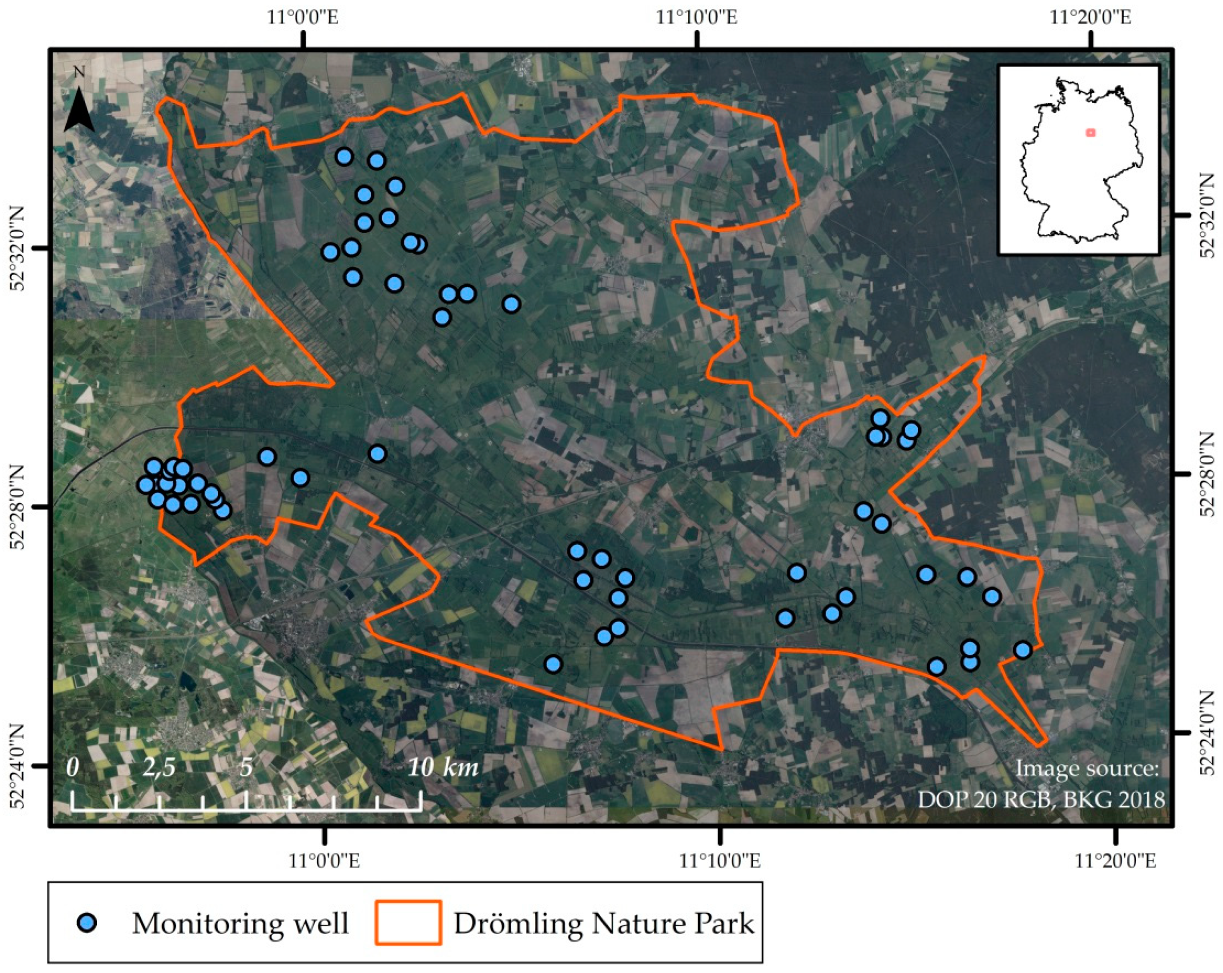
2.1. Study Area

The Drömling is a lowland landscape in the German federal states of Saxony-Anhalt and Lower Saxony. In Saxony-Anhalt, large parts of the Drömling are protected as a nature park, which comprises several nature reserves [32]. Fen peat developed between sand islands deposited by the Aller and Ohre rivers. Due to the flat topography and the underlying sand, horizontal hydraulic gradients are small, i.e., the groundwater surface is rather flat. Therefore, it can be assumed that the absolute level of the water table measured at one point is representative for a larger area.

The area has been cultivated and systematically drained for agricultural purpose since the late 18^th century. Additionally, parts of the Drömling peatlands have been covered by sand to improve trafficability (‘Rimpau’sche Moordammkultur’). Due to peat mineralisation and subsidence caused by drainage, the peat depth is shallow nowadays (from ~15 to 60 cm) and large areas are at the boundary between mineral and organic soils in terms of their organic carbon content. Land parcels are small with numerous ditches as well as shrubs and trees next to the fields. In the last few decades, the area of cropland has decreased and conversion of grassland to cropland has been banned to reduce land-use intensity and to support conservation efforts in the core zone of the park [31]. Currently, most of the area is used as grassland with low intensity management (73% in 2012 [31]).

Long-term mean precipitation and temperature are 560 mm and 8.7°C, respectively [33]. During summer, evapotranspiration frequently exceeds precipitation and groundwater inflow, which can result in low water tables of around 1 m. In some parts of the Drömling, re-wetting measures have been implemented to raise the water table, but inundation only occurred at a few sites during the investigated time period in winter.

The study area was chosen because it is data-rich, i.e., WTD has been monitored in the Drömling area of Saxony-Anhalt (eastern part) at about 100 monitoring wells. We focused our analysis on grassland because this is the major land use type for both the Drömling [31] and organic soils in Germany in general [5,7].

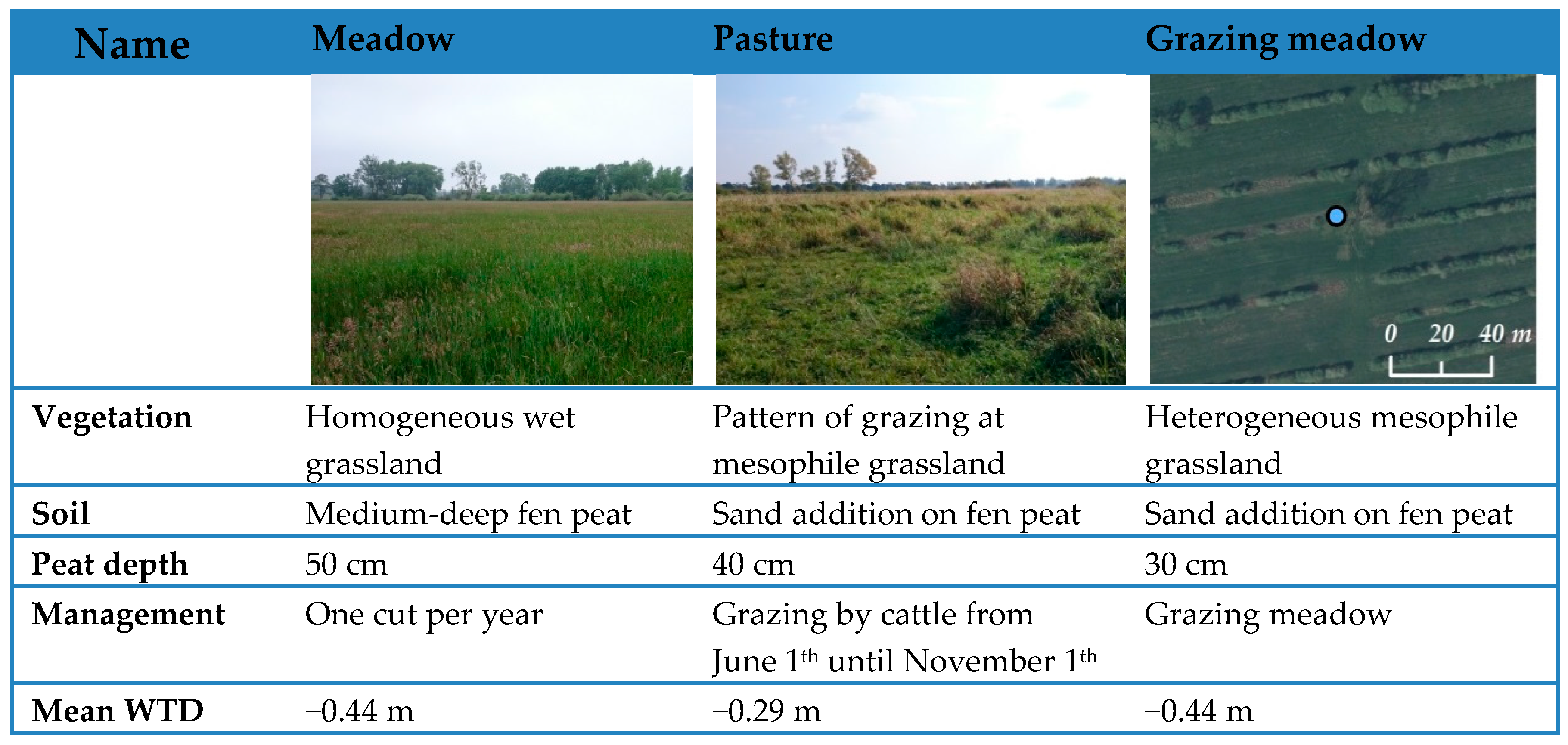
2.2. In Situ Data: Water Table, Soil and Vegetation

In total, 60 monitoring wells (Figure 2) were used to obtain in situ data for a correlation analysis between WTD and σ⁰ using a change detection approach.

For comparison with σ⁰, the study sites were defined as an area of 130 m × 130 m around the monitoring wells. These dimensions were derived from pre-tests that aimed at finding an appropriate speckle filter size (details in Section 2.3.2). Study sites are situated all over the Drömling in grassland parcels with differently managed water levels, and thus they differ in mean WTD, vegetation type and soil properties. The available length of time series overlapping with our analyzed Sentinel-1 period differ among the monitoring wells and range from 365 to 787 days, although the time period is mostly about two years long. Mean annual WTD of the study sites ranged from −0.80 to −0.05 m (negative = below ground surface).

Information on ground elevation was derived from a digital elevation model (DEM). The DEM is based on an airborne laser scan from 1998 and has a spatial resolution of 5 m and a height uncertainty of 0.08 m [34]. After 18 years, soil subsidence due to peat mineralisation has to be expected. Therefore, we measured the current ground elevation at several study sites and found that the peat surface was around 10 cm lower than indicated by the laser scan. Thus, the DEM was corrected accordingly. WTD was derived by subtracting the ground elevation (mean of the 130 m × 130 m area) from water table elevation. Precipitation and soil temperature at a 5 cm depth were measured hourly at the climate station of the German Weather Service in Gardelegen, which is about 18 km from the study area.

Soil information was supplied by the Nature Park administration, who conducted a detailed field mapping. Main soil types are shallow (up to 0.60 m) Histosols with strongly decomposed fen peat, Histic Gleysols and sand-covered Histosols [35]. Soils that have very shallow or no peat but a high SOC content such as Histic Gleysols are referred to below as “other organic soils”. Study sites are further classified by peat depth (medium-deep fen peat for depths > 0.40 m and shallow fen peat for depths < 0.40 m).

All study sites are grasslands managed with low intensity (one or two cuts per year, low intensity grazing). Recent information on vegetation was available from field mapping campaigns in 2016, according to the habitat classification approach of the EU Habitat Directive [36] and to the biotope type classification (BTC) in Lower Saxony [37]. However, as these maps covered only parts of the study area, biotope type groups based on colour-infrared (CIR) data from 2009 were used in case of missing information [38]. In both cases, information for each study site was extracted with a rectangular buffer of 130 m representing the area of the adapted speckle filter. While the CIR-based map only contains coarse classes of vegetation, detailed subclasses were available from the more recent data. We decided to subdivide the vegetation into broad classes: wet grassland (n = 19), sedges (n = 1) and mesophile grassland (n = 34) with the subclass of lowland hay meadow (n = 6) (details in

Table A1. Established vegetation classes and their subclasses from habitat mapping (HTC) and biotope type mapping (CIR + BTC) [36,37,38].

Vegetation Class	Description	Name of Subclass	Habitat Types Code	Biotope Types Code
Mesophile grassland	Moderately dry to moderately wet nutrient-rich sites	Mesophile grassland	GMA	GM
		Other mesophile grassland		GMX
Lowland hay meadow	Extensively managed, species-rich hay meadows rich in flowers	Lowland hay meadow	6510	6510
Wet grassland	Moderately wet to wet grassland, extensively used or fallow	Wet grassland		GF
		Fallow of wet grassland	GFX
		Periodically flooded grassland	GFE
		Other wet grassland	GFY	GF
Sedges	Mainly sedges at wet sites	Sedges	NSD

).

Vegetation biomass changes seasonally and annually not only due to climatic conditions, but also due to differences in management. The parcels within the study sites are either cut once or twice a year, used as pasture (usually for cattle) or a combination of both. To complicate matters, a few parcels are cut in alternating strips for conservation purposes. Management decisions depend on hydro-meteorological conditions (e.g., trafficability, which is understood here as the soil’s ability to support agricultural traffic without major soil degradation) and on conservation goals (e.g., the date of the first cuts is optimized for breeding birds). However, detailed management information was only available for a few sites.

Three exemplary study sites were chosen to demonstrate the time series of σ⁰ and WTD, but management data was only available for two of these (Figure 3). The first study site (Meadow) had quite homogeneous wet grassland vegetation, which reached a height of about 1.4 m in 2016. At the second study site (Pasture), around 20 cm of sand has been added on the top of the peat layer and the upper layer is now a peat-sand mixture. The vegetation and its biomass vary on a small scale due to inhomogeneous grazing of cattle. The third study site (Grazing meadow) is similar to the second, but with generally higher vegetation and small strips of shrubs around ditches. The Grazing meadow serves as an example of those sites that show a weak correlation between WTD and σ⁰ (Section 3.3).

2.3. Sentinel-1 Data

2.3.1. Data Availability and Scene Filtering

Data products from Sentinel-1 satellites were downloaded from the Copernicus Open Access Hub [39] for the study period from October 2014 to December 2016. The products were processed as Level-1 data from Interferometric Wide Swath Mode (IW) and Ground Range Detected (GRD). All available scenes (in total 262) from Sentinel-1A and Sentinel-1B were used. Two polarization products were available with vertical transmission and either vertical reception (VV) or horizontal reception (VH). The posted raster cell size of the data products was about 10 m × 10 m. The scenes were received from four different orbits. Scenes differ in viewing direction, incidence angle (depending on the orbit, either about 35°or 43° for the study area) and sensing time (either in the morning at 06.00 CET or in the evening at 18.00 CET). Because of the different viewing geometries, scenes were divided into ascending and descending orbits. To ensure (as much as possible) the hydrostatic (+ unfrozen) equilibrium condition that is the basis of the direct monitoring of WTD with backscatter data, we tested various thresholds for soil temperature and time since last precipitation. The rationale of the latter is that precipitation just before the overpass would lead to high backscatter values due to a temporary wetter surface layer, which is poorly connected to the current water table position. We found that a 2°C threshold and a rain-free period of 6 h successfully filtered outliers that otherwise blurred our correlation coefficients. Therefore, only scenes of dates where the soil temperature was higher than 2°C and no precipitation occurred at the weather station for the last six hours were used. Filtering reduced the number of analyzed scenes to 144.

2.3.2. Data Processing

The radar data were pre-processed with ESA’s Sentinel-1 Toolbox in the software SNAP (Version 6.0) [40]. The processing routine included thermal noise removal. For geocoding precise orbit files and the Range-Doppler Terrain Correction was applied. Input data for the terrain correction is the German digital terrain model with a raster width of 25 m with adjusted elevation from German Combined Quasigeoid. Sentinel-1 raster cells were transformed to represent an area of 10 × 10 m on the ground. The digital numbers of the raster were radiometrically calibrated to the radar cross-section σ⁰ in decibel and are hereafter referred to as σ⁰ backscatter coefficients, or just σ⁰.

Areas of forest, croplands and permanent open water bodies in the study area were masked by the CIR map to avoid influences on σ⁰ at the study sites. After that, a median window speckle filter with a size of 13 × 13 raster cells was applied. The filter reduces small scale differences due to speckle but also heterogeneities within the grassland. The filter size was chosen after pre-tests as a compromise between smoothing smaller scale heterogeneities and resolving abrupt changes between differently managed parcels. For three study sites, backscatter values were masked within the study sites during the application of the land use mask. Missing values for these study sites were extrapolated during speckle filtering up to half of the speckle filter size.

For each study site and both polarizations, σ⁰ was extracted at the position of the monitoring wells. They were further analyzed in R (Version 3.4.3) [41]. Additional information on incidence angles for each study site and scene were extracted from the Sentinel-1 incident angle raster of the product.

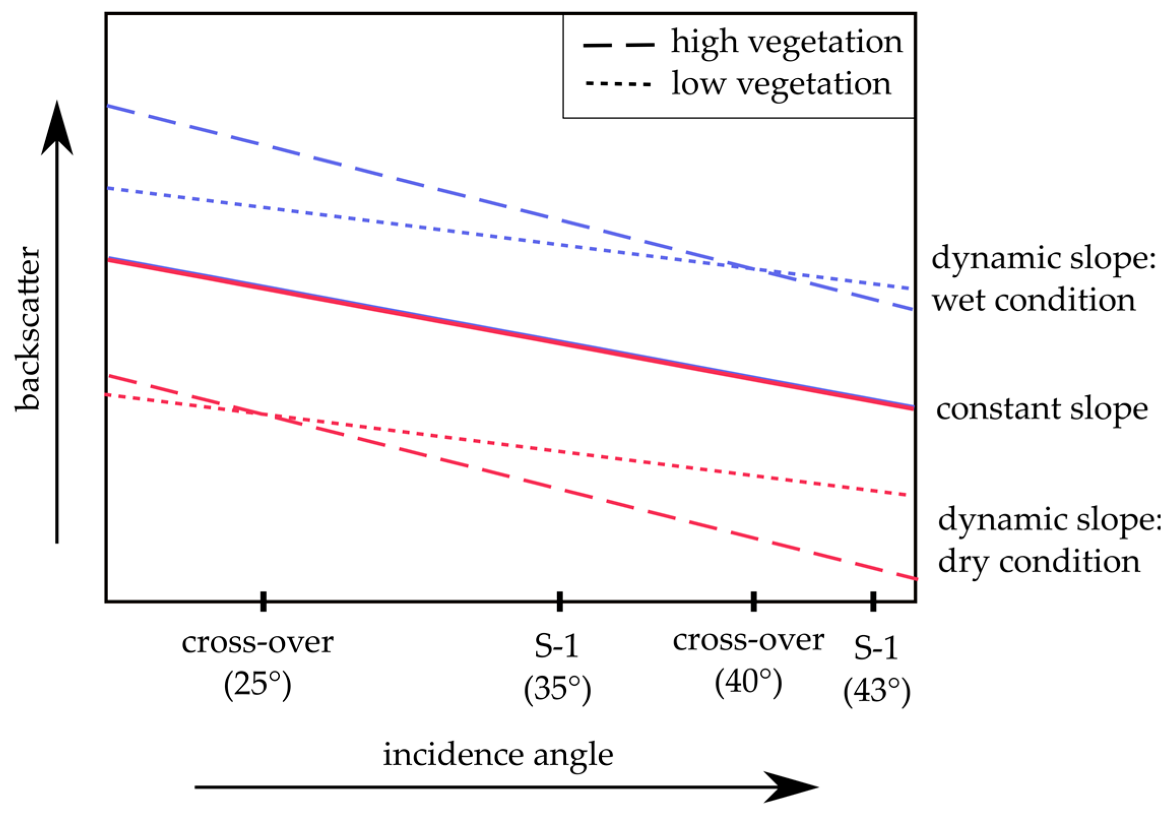
2.3.3. Derivation of Slopes of σ⁰ Incidence Angle Dependency

All σ⁰ were normalized to a reference angle of 40° with a constant and a dynamic slope according to the cross-over angle concept [19]. Since only two incidence angles are available for Sentinel-1 satellites, information on curvature cannot be derived. Therefore, the cross-over angle concept is applied in a simplified manner neglecting the effects of dynamic vegetation on the curvature of the incidence angle dependency [42]. The slope is supposed to account for the major effects of seasonal vegetation development. The constant slope was calculated as the mean slope between σ⁰ and incidence angle from two complete years of Sentinel-1 data (Figure 4). The dynamic slopes, which represent the climatology of the area, were derived according to Bechtold et al. [29]. For each day of a year, the slope was derived with a moving average window. Weighting of the scenes accounted for irregular incidence angles inside the moving window. The cross-over angle concept was only applied to VV polarization because it showed a better correlation with WTD in pre-tests. Normalized σ⁰ will be referred to as ${\sigma }^0{}_{\theta }$, with ${\sigma }^0{}_{\theta }$ constant and ${\sigma }^0{}_{\theta }$ cross-over referring to the constant and cross-over angle method, respectively.

As a further indicator of vegetation development, the polarization difference (PD) was calculated as

$$\mathrm{PD}\mathrm{constant}={\mathsf{\sigma }}^0{}_{\mathsf{\theta }}\left(\mathrm{VV}\right)\mathrm{constant}-{\mathsf{\sigma }}^0{}_{\mathsf{\theta }}\left(\mathrm{VH}\right)\mathrm{constant}$$

(1)

2.3.4. Correlation Analysis

We applied a correlation analysis to evaluate the potential of backscatter time series for WTD monitoring. Simple univariate correlation coefficients between backscatter (or soil wetness indices derived from scaled backscatter) and soil moisture are frequently reported in the remote sensing of soil moisture field [43,44]. Since WTD and ${\sigma }^0{}_{\theta }$ dependencies were slightly nonlinear for several study sites, correlation coefficients were calculated using Spearman rank correlation, as done, e.g., in Dorigo et al. [43]. The correlation coefficients are not independent from vegetation changes. To account for vegetation as a confounding factor, we calculated partial correlation coefficients between ${\sigma }^0{}_{\theta }$ (VV) constant and WTD after [45] with the effect of the controlling random variable PD, as proxy for vegetation, removed. For all correlation analysis, dates with a WTD shallower than −0.05 m were excluded from the calculation of correlation coefficients because a partly inundated ground surface would lead to a contrary relationship between σ⁰ and WTD (Figure 1). To separate the effects of soil properties, vegetation types or the general wetness level (mean WTD) on the correlation coefficients, we classified study sites by these characteristics. The distance to ditches, trees, shrubs and open water bodies was tested for their effect on the correlation.

3. Results

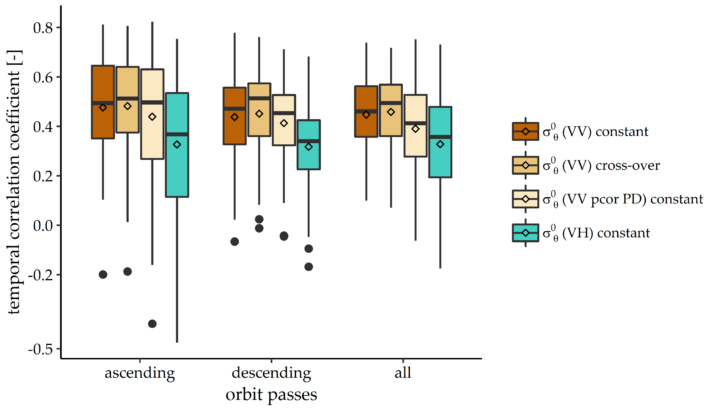
3.1. Influence of Polarization, Incidence Angle Normalization and Orbit on the Correlation of WTD and Backscatter

Figure 5 summarizes the correlations between the various backscatter variables and WTD. On average, the orbit pass (ascending/descending) did not systematically affect correlations. Combining both orbits, the highest mean correlation coefficient (0.46) was achieved with VV polarized σ⁰ with cross-over angle normalization directly followed by VV polarized σ⁰ with constant slope normalization (0.45). Partial correlation analysis indicates a slight decrease in the correlations between VV polarized ${\sigma }^0{}_{\theta }$ and WTD (shown for ${\sigma }^0{}_{\theta }$ constant only). VH polarization showed a correlation coefficient of only about 0.32.

The application of the cross-over angle principle increased the mean correlation coefficient by, on average, only 0.01. However, the moving window approach yielded mostly plausible slope parameter climatologies, although only two different incidence angles were available (Figure 6). The slope value increased during summer, i.e., during periods with high vegetation biomass (see also Figure 4). One exception was a study site with a vegetation cover dominated by sedges, which did not show the expected pattern (Figure 6d). Longer time series are necessary to evaluate whether this pattern is consistent over time. It can be further noted that differences between the vegetation classes, mesophile grassland and wet grassland were very small. However, wet grassland had greater quantile values, which might point to greater diversity between the study sites.

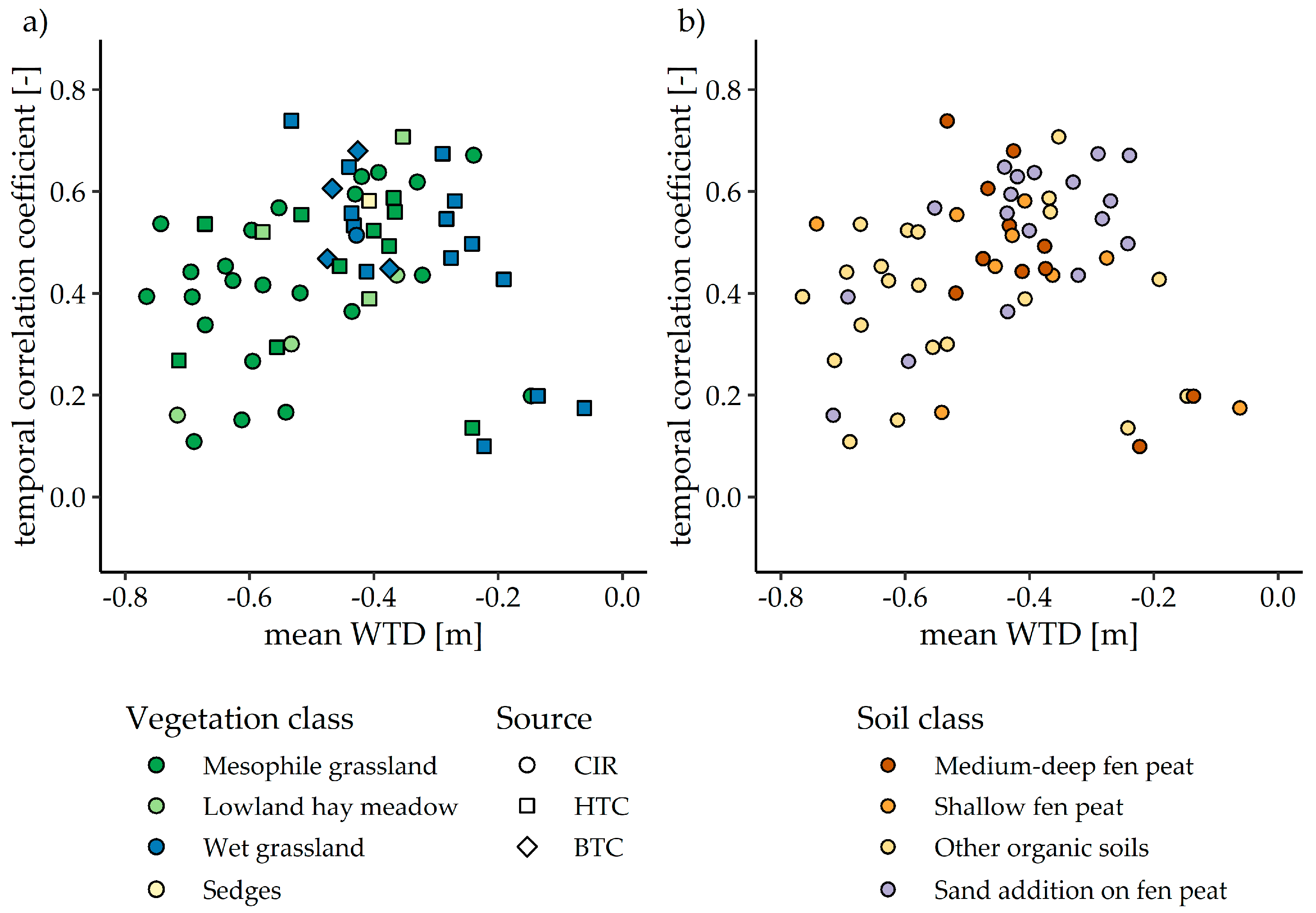
3.2. Influence of Mean WTD, Vegetation and Soil on the Correlation between WTD and Backscatter

Since the cross-over angle correction had only a minor impact, the following analysis is restricted to the σ⁰_ϴ (VV) constant data from both orbits. Overall, study sites showed a large variability in correlation coefficients (0.10–0.74). Figure 7 illustrates the temporal correlation coefficients for all study sites classified by the main vegetation class (Figure 7a) and soil class (Figure 7b). It can be observed that both very dry and very wet study sites had lower correlation coefficients, while there seemed to be an optimum at a mean WTD of around −0.40 m. Accordingly, the drier study sites of the wet grassland and the wetter study sites of the mesophile grasslands and lowland hay meadows showed relatively high correlation coefficients. In the range where the mean WTD of the vegetation classes overlap (−0.50 to −0.30 m), there was no systematic influence of the vegetation class. Overall, the results indicated that correlation coefficients were influenced by the general “wetness level” of a site, i.e., the mean WTD.

As expected, the class of other organic soils generally showed deeper mean WTD than study sites with fen peat (Figure 7b). However, while the correlation decreased with deeper mean WTD (Figure 7b) within the soil classes, there were no systematic differences between the soil classes. Independent of vegetation and soil class, correlation coefficients were low at shallow mean WTD, even though inundation events were excluded from the analysis and a considerable range of WTD fluctuations (>0.6 m) was still present for every site.

It should be noted that even at similar mean WTD, there was a large range of correlation coefficients. We analyzed features of footprint heterogeneity such as the distance to shrubs, open water, wood or more detailed habitat types (data not shown), but critical factors governing the strength of the correlation between WTD and σ⁰ could not be identified. Furthermore, we observed a high and WTD-independent variability in the absolute values of σ⁰ across different study sites that could also not be explained by the aforementioned site factors (Figure S1).

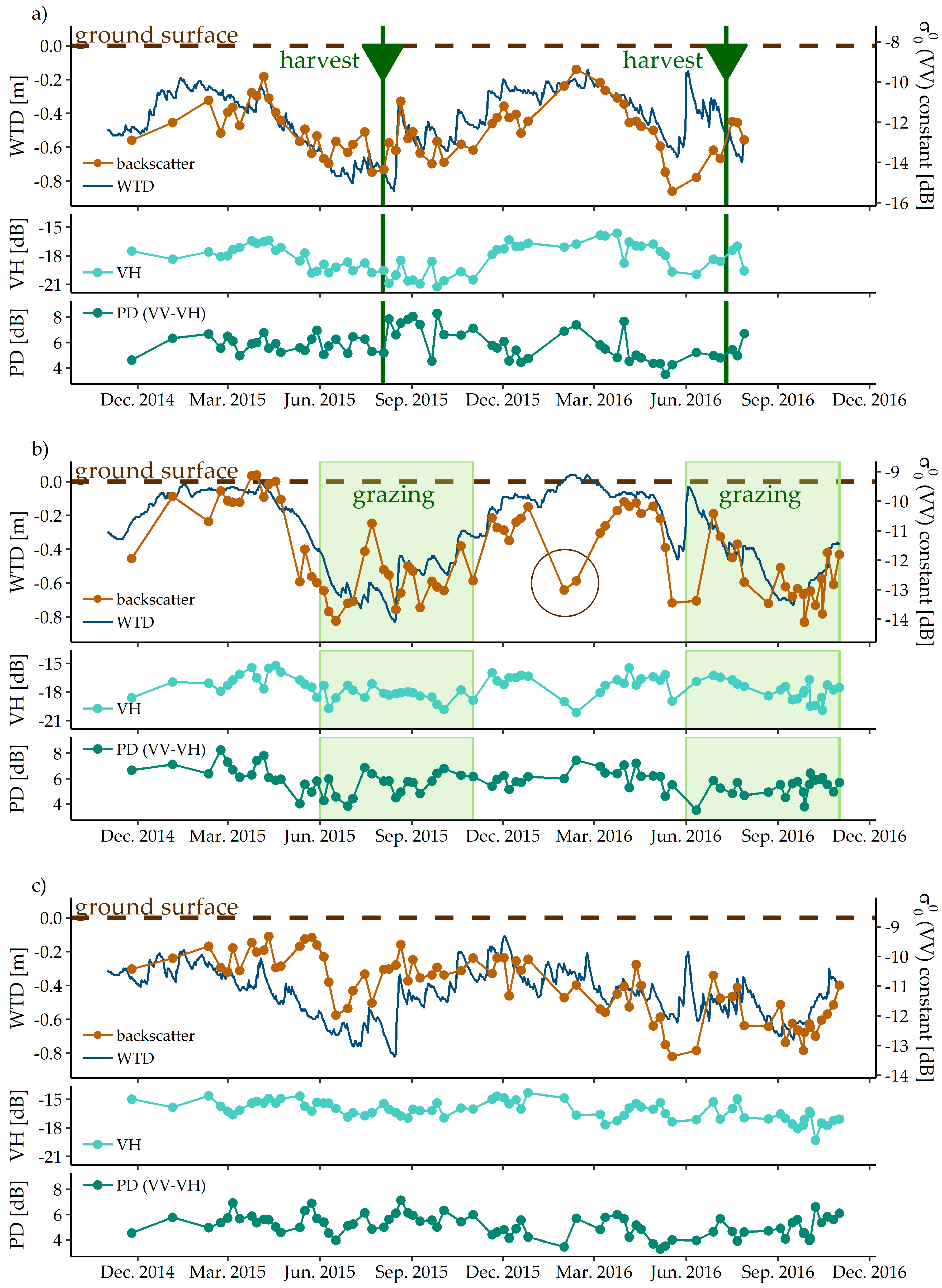
3.3. Exemplary Time Series: Influence of Grassland Management Activities

As described above, the dynamics of σ⁰ tracked the WTD dynamics well at some sites, while at others there was a very weak correlation. At the first exemplary study site (Meadow) in Figure 8a, σ⁰ matched several rises in water level but the dependency was weaker in summer. However, there were considerable differences between the two summer periods; in 2015, the σ⁰ dynamics matched the WTD well, especially after the harvest (grass cut), while in June 2016 one major rise in WTD could not be captured by the σ⁰ time series. This might be explained by the high vegetation biomass at the time of the WTD rise because in that year, the harvest took place after a major increase in WTD.

At the grazed study site (Pasture) in Figure 8b there was, in general, a stronger correlation between σ⁰ and WTD throughout the summer, which might be due to generally shorter vegetation due to grazing. Grazing took place from 1 June until 1 November. The WTD rise in summer 2016, which was not captured by σ⁰ at the Meadow site, could be observed in the σ⁰ time series of the Pasture site.

Inundation of the grazed site in February 2016 led to a drop in σ⁰ (marked by a circle in Figure 8b). This study site was one of the very few sites where inundation occurred. It should be noted that σ⁰ during inundation are similar to σ⁰ during very dry conditions.

Figure 8c shows a representative example of a study site (Grazing meadow) with a low correlation coefficient (r = 0.37) even at an intermediate mean WTD (−0.44 m), for which we observed most of the highest correlation coefficients. The management and soil properties are quite similar to the Pasture site, but the speckle filter window of the Grazing meadow study site is fragmented into several very small parcels and, despite grazing, we observed high vegetation during a field campaign in summer 2016. Furthermore, there are many ditches (every 20 m) surrounded by shrubs at this site. It might be the combination of all these potentially confounding factors that lead to the weak correlation, as one factor alone (e.g., high ditch density) did not explain low correlation coefficients at other sites.

For the shown time series, we could (visually) not identify direct connections between seasonal or management-induced changes in vegetation characteristics and the time series of PD and VH (Figure 8a,8b,8c).

4. Discussion

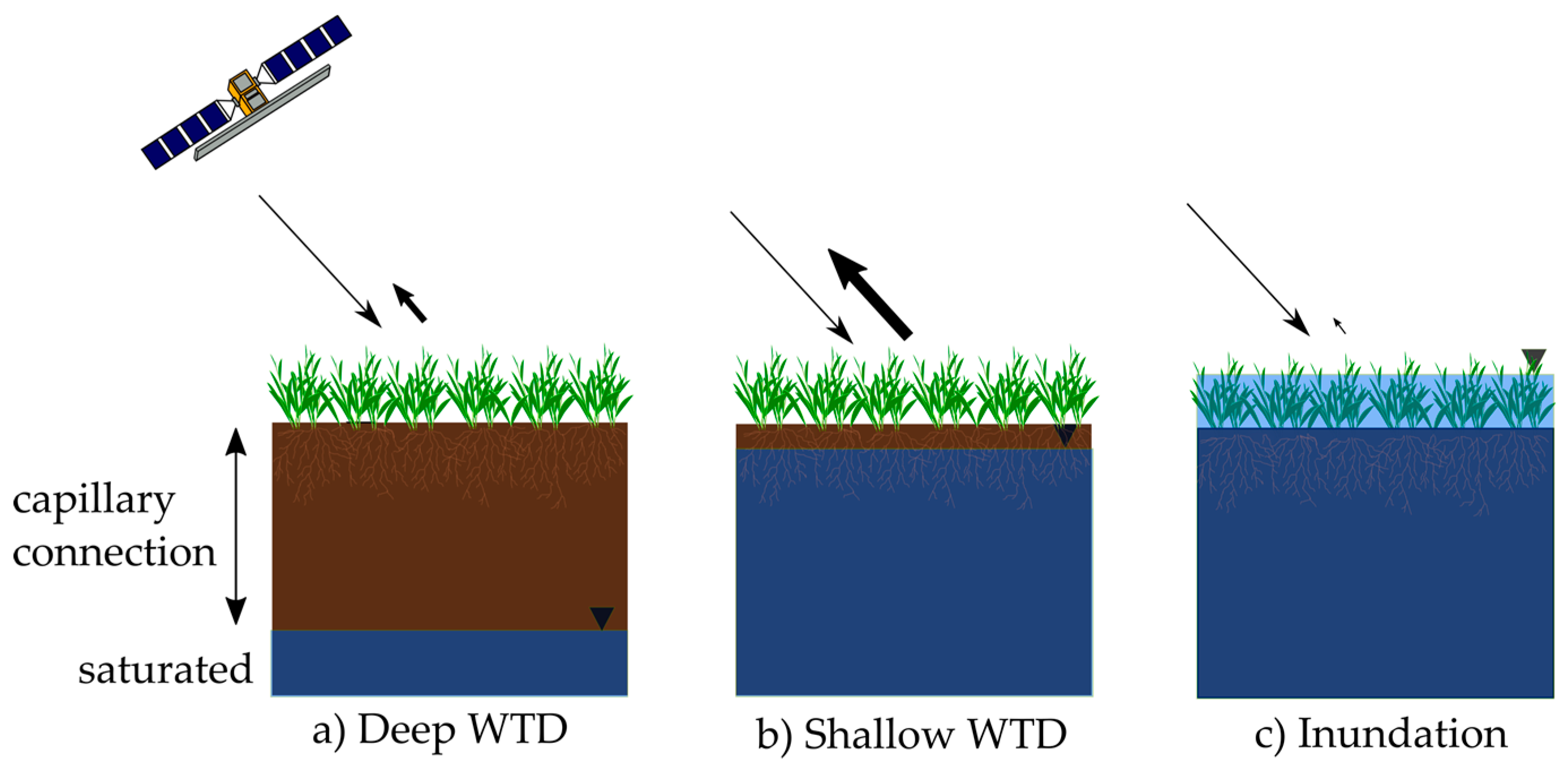
4.1. General Dependency of Backscatter on WTD

Our study demonstrated a dependency of Sentinel-1 σ⁰ on WTD in a drained temperate peatland with degraded organic soils used as extensive grassland (Figure 5), as previously shown by Kim et al. [28] in a forested peatland for Radarsat-1 data and by Bechtold et al. [29] for ENVISAT ASAR data across several study sites in Germany. We emphasize that the organic-rich soil in our study area was highly degraded, and, thus, showed rather high surface soil moisture despite the (for natural peatlands) rather deep WTD. The dependency of σ⁰ on WTD was, therefore, likely stronger and less complex than in other studies on organic soils with a fibric undecomposed organic-rich soil surface layer for which confounding effects can occur due to considerable subsurface scattering [46,47]. The derived correlation coefficients of our study were similar to the results of Bechtold et al. [29] who found mean correlation coefficients between 0.42 and 0.47 with VV polarized ENIVSAT ASAR data. Overall, the derived coefficients were also comparable to correlations between σ⁰ and peat soil moisture determined by Dabrowska-Zielinska et al. [25]. For drained organic soil used as intensive grassland, these authors showed a decrease in the correlation with increasing soil moisture sensing depth (from 5 to 20 cm), though moderate correlation coefficients between 0.26 and 0.55 were still derived for soil moisture at a 20 cm depth. The partial correlation analysis with PD as the controlling variable and proxy for aboveground biomass [25] indicates that VV remains correlated to WTD even considering biomass as a confounding factor.

Similarly to Bechtold et al. [29], the use of the cross-over method improved the correlation coefficients only marginally compared to constant slopes. The uncertainty of the dynamic slope parameter probably limited the potentially higher benefit of the cross-over angle concept. Two years of Sentinel-1 data is a short timeframe and it was insufficient to cover different moisture states at the different incidence angles, which only covered a narrow incidence angle range of 8° over our study area and thus further hindered a reliable derivation. Additionally, abrupt vegetation changes due to management activities are problematic since the current approach relies on smooth climatologies of the slope of the incidence angle dependency. Furthermore, it is unclear whether the current globally applied cross-over angles used for the cross-over angle concept, which were originally derived over the Iberian Peninsula [19] and never adapted, are optimal for peatland conditions in Central Europe (see discussion in [29]). A direct derivation of the cross-over angles from data as done in [19] is not possible due to the general lack of conditions in drained peatlands whereby high water tables and high vegetation biomass occur simultaneously [29]. Such conditions would be necessary to constrain the wet reference (Figure 4). In our study area, an additional limiting factor is that only two different incidence angles were available, which covered only a small range (35° and 43°) whereas previous studies used data with several (15° to 45°) incidence angles [19,29,48].

Lower correlation coefficients for VH polarization are consistent with other studies on soil moisture estimation from σ⁰ and confirm the assumption that VH is more dependent on volume scattering in the vegetation [49]. If VH were well related to vegetation cover it would be advantageous to integrate information on VH or PD into the results of σ⁰ (VV). As a substitute for NDVI, PD was used by Dabrowska-Zielinska et al. [25] as a parameter for vegetation in a soil moisture retrieval model. At a global scale, Greifeneder et al. [49] showed that the integration of PR (polar ratio, which has similar information content as PD) into a soil moisture change detection model in addition to the cross-over angle method, improved the correlation between soil moisture and σ⁰ for individual study sites, but not for the whole data set. There is a need to conduct in-depth polarimetric investigations on the basis of more detailed vegetation information than that available for our study sites to detect the systematic effects for managed peatlands.

4.2. Influence of Mean WTD and Soil Properties on Correlation

At our sites, the mean WTD exerted the strongest influence on the strength of the correlation between WTD and σ⁰ (Figure 7). In the dry range, the observed loss of correlation is similar to the findings of Akbar et al. [50] who analyzed SMAP data and found a weak link between observed surface soil moisture and soil moisture from deeper layers for drier geographical regions. For our shallow water table conditions, there are at least two mechanisms that could cause a decrease in correlation for sites with deeper mean WTD. First, surface soil moisture (and thus backscatter) variations might be diminished for deep WTD fluctuations due to the insensitivity of the corresponding drier sections of the soil water retention curve. This effect is supported by our available soil hydraulic information. A surface soil sampling of ten study sites and subsequent laboratory experiments using methods tested and optimized for peat samples [3,51] indicated that we can assume about 35% less change in surface water content for water table changes at −0.7 than at −0.4 m (Figure 9). As a second mechanism, lower correlation coefficients at study sites with deeper mean WTD might also be explained by a loss of hydrostatic equilibrium, that is, by the loss of the strong capillary connection between the water table and the “sensed” surface soil layer. The occurrence of disequilibrium conditions becomes more likely with deeper WTD.

Given that deep water tables occur during summer in most cases, when vegetation biomass is highest, it is problematic to analyze loss of sensitivity (backscatter/surface moisture to WTD) further at the level of single sites. For periods with low vegetation biomass, the amount of data for deep water tables is insufficient to evaluate the loss of sensitivity without the very confounding effect of a mostly dense summer vegetation layer. We emphasize that our interpretation of the loss of sensitivity with deeper WTD is only based on multi-site analysis using site-specific mean WTD.

We further expanded soil physical considerations using the available soil maps. Soil physical properties may vary strongly between different peat types and degradation stages [9,52,53], but we did not detect any differences in correlation for different soil classes at the same WTD. Originally, we expected differences between sandy topsoils, which drain at lower suctions and lose capillary connection earlier and peat topsoils, which are supposed to have a capillary connection over a wider WTD range. The fact that we did not observe this effect might be related to an unmapped variability in the soil properties within the 130 × 130 m squares (the definition of a study area). It is also possible that differences in physical properties between the soil classes are simply too small to have notable effects at this spatial scale. This might not be true at larger scales or when comparing different peatlands as the soil properties (strongly degraded fen peat and other organic soils) and the peat depth (generally rather shallow) of the study area only cover a small range of peat properties and depths occurring at a larger spatial scale. Another factor that might mask any potential effects of the soil type is the presence of silty organic sediments (sedimentary material deposited at the bottom of water bodies before the onset of peat formation) within the unsaturated zone. Such occurrences were sporadically encountered in some soil profiles at depths of 30 to 50 cm and these may alter the capillary connection between the topsoil and water table.

The decrease in correlation coefficients at the highest mean WTD (Figure 7) might be due to small-scale microtopography, which causes local ponding under wet conditions. Such periods might not be well filtered by our WTD threshold of −0.05 m. One of the exemplary time series (Figure 8b) clearly shows that even shallow inundation has a crucial influence on σ⁰. Most inundation events occur during winter when the vegetation of our managed grasslands is low and the inundation water is only sparsely covered by vegetation. Under these conditions, a decrease in σ⁰ can be expected [15,17], and probably explains why we did not observe an increase in backscatter due to the double bounce effect, as in [28]. The detection of flooded areas could improve water management and the estimation of GHG emissions. However, a precise method to distinguish inundated vegetation from deep WTD is needed because both situations have strong, but opposite effects on GHG emissions—low groundwater tables cause high emissions of CO₂, while lasting inundation (particularly in summer) might cause high methane (CH₄) emissions from both grassland [5] and re-wetted sites [54]. Inundation during winter, however, is generally less problematic. A challenge will be to account for small-scale inundation patterns under vegetation [55] throughout the different parts of peatlands and to develop a reliable method for a variety of sites. However, this would be needed if CH₄ emissions were the focus of a particular project or if re-wetting measures are to be identified at the larger scale.

4.3. Influence of Vegetation on Correlations and Backscatter Time Series

Whereas the different vegetation classes show no distinguishable influence besides the correlation to mean WTD, abrupt changes in biomass due to management cannot be captured by the current cross-over angle method based on a moving window approach. In many peatlands and also in the Drömling, management strongly depends on hydro-meteorological conditions, which makes averaging across years more problematic than with unmanaged land. Dynamic characterization of the incidence angle dependency that resolves inter-annual variability, as for Metop ASCAT data [56], is hardly obtainable from the limited incidence angles of the Sentinel-1 configuration. Theoretically, supplementary information (e.g., harvest dates) on vegetation could be used to improve the moving window approach and to account for management, although management practices with regard to grassland in Germany are highly variable and difficult to obtain at a parcel scale. Approaches to estimate cuts on grassland from remote sensing data include, e.g., the use of coherence data [57] and optical data from Sentinel-2 [58]. However, due to cloudiness, there were not enough scenes from Sentinel-2 during the study period to test such an approach. In future, the necessary information might be derived from other satellite data, but currently, in situ data remains irreplaceable and sparse.

WTD at grazed sites might be easier to predict because of both lower vegetation and no abrupt changes in vegetation height. High biomass has been shown to reduce the accuracy of predicting soil moisture [59], showing a decrease in correlation for the summer months [25]. Although grazed sites might be very inhomogeneous due to the fodder preferences of the cattle (as we have noticed during several site visits in summer 2016), this heterogeneity might have been smoothed by the use of a relatively large speckle filter. However, to conclude on whether and/or to what degree high vegetation or non-equilibrium soil water conditions are responsible for weaker correlations between σ⁰ and WTD during summer, more detailed information on grassland management and the additional monitoring of surface soil moisture is needed.

5. Conclusions

In this study, we evaluated for the first time, the correlation between high spatial resolution (here 130 m) Sentinel-1 σ⁰ and water table depth (WTD) in drained (and thus degraded) organic soils (partly peatlands) with grassland management. Averaged over 60 monitoring sites, the temporal Spearman correlation coefficient between σ⁰ and WTD was 0.45. The highest correlations were found for sites with a mean annual WTD of around −0.40 m. For sites with a mean annual WTD deeper than appr. −0.60 m or shallower than appr. −0.20 m, we observed a clear decrease in correlation. A reduced surface soil moisture variability for deeper WTD changes (still assuming hydrostatic equilibrium conditions) and the potential loss of the capillary connection between the water table and the surface soil layer (penetrated by the microwaves) during dry periods (assuming disequilibrium conditions) are two potential explanations for the reduced correlation at the drier sites. At the wettest sites, the correlation is possibly influenced by periods of partial inundation during which specular reflection reduces σ⁰. The reduced correlation in very dry and very wet sites can be considered as a potential limit in the application of σ⁰ for WTD monitoring at high spatial resolution. This observation could not be made in a similar previous study [29], in which much coarser σ⁰ data from ENVISAT-ASAR was analyzed, and thus, higher sub-resolution heterogeneity of WTD occurred.

In order to use Sentinel-1 σ⁰ for upscaling GHG emissions from organic soils in which WTD is a key parameter [5,60], three challenges should be addressed in future research. First, a method is needed to resolve the observed ambiguity of low σ⁰ from deep WTD (high CO₂ emissions) and partial inundation in the course of re-wetting measures (low CO₂ emissions or even uptake, but potentially high CH₄ emissions). Second, tall vegetation during summer needs to be addressed, either corrected for or masked, because it might cause the correlation between σ⁰ and WTD to completely disappear. The integration of management and vegetation data (e.g., harvest dates, estimates of vegetation height or biomass) could improve (i) the identification of periods with applicable σ⁰ data, and/or (ii) the cross-over angle method that, in our study, only slightly increased the correlation between σ⁰ and WTD compared to a simple constant slope incidence angle correction. Third, the absolute level of σ⁰ varied strongly across sites, which makes the estimation of absolute WTD and the spatial transferability of correlations impossible at the moment. A stratification of the study sites by vegetation and soil class did not yet help in this regard.

Despite the above challenges, the obtained correlation between σ⁰ and WTD suggests the direct use of Sentinel-1 σ⁰ in a data assimilation framework, as done in [61] in order to improve estimates of WTD fluctuations, provided that the framework addresses the peatland-specific hydrology with an adequate land surface modelling concept [62], including a drainage component for the land fraction of drained organic soils.

References

1. Yu, Z.; Loisel, J.; Brosseau, D.P.; Beilman, D.W.; Hunt, S.J. Global peatland dynamics since the Last Glacial Maximum. Geophys. Res. Lett. 2010, 37, L13402. [Google Scholar] [CrossRef]
2. Boden, A.G. Ad-hoc-AG Boden Bodenkundliche Kartieranleitung KA5, 5th ed.; Schweizerbart: Hannover, Germany, 2005; pp. 257–263. [Google Scholar]
3. Dettmann, U.; Bechtold, M.; Viohl, T.; Piayda, A.; Sokolowsky, L.; Tiemeyer, B. Evaporation experiments for the determination of hydraulic properties of peat and other organic soils: An evaluation of methods based on a large dataset. J. Hydrol. 2019, 575, 933–944. [Google Scholar] [CrossRef]
4. Paavilainen, E.; Päivänen, J. Peatland Forestry: Ecology and Principles; Ecol. Stud. 111.; Springer: Berlin/Heidelberg, Germany, 1995. [Google Scholar]
5. Tiemeyer, B.; Albiac Borraz, E.; Augustin, J.; Bechtold, M.; Beetz, S.; Beyer, C.; Drösler, M.; Ebli, M.; Eickenscheidt, T.; Fiedler, S.; et al. High emissions of greenhouse gases from grasslands on peat and other organic soils. Glob. Chang. Biol. 2016, 22, 4134–4149. [Google Scholar] [CrossRef] [PubMed]
6. Wilson, D.; Blain, D.; Couwenberg, J.; Evans, C.D.; Murdiyarso, D.; Page, S.E.; Renou-Wilson, F.; Rieley, J.O.; Sirin, A.; Strack, M.; et al. Greenhouse gas emission factors associated with rewetting of organic soils. Mires Peat 2016, 17, 4. [Google Scholar] [CrossRef]
7. Umweltbundesamt. Submission under the United Nations Framework Convention on Climate Change and the Kyoto Protocol 2018 National Inventory Report for the German Greenhouse Gas Inventory 1990–2016; Umweltbundesamt: Dessau-Roßlau, Germany, 2018. [Google Scholar]
8. Arets, E.J.M.M.; Van Der Kolk, J.W.H.; Hengeveld, G.M.; Lesschen, J.P.; Kramer, H.; Kuikman, P.J.; Schelhaas, M.J. Greenhouse Gas Reporting for the LULUCF Sector in the Netherlands Methodological Background, Update 2018; Wageningen University and Research: Wageningen, The Netherlands, 2018. [Google Scholar]
9. Dettmann, U.; Bechtold, M. Deriving Effective Soil Water Retention Characteristicsfrom Shallow Water Table Fluctuations in Peatlands. Vadose Zone J. 2016, 15, 1–13. [Google Scholar] [CrossRef]
10. Dettmann, U.; Bechtold, M.; Frahm, E.; Tiemeyer, B. On the applicability of unimodal and bimodal van Genuchten-Mualem based models to peat and other organic soils under evaporation conditions. J. Hydrol. 2014, 515, 103–115. [Google Scholar] [CrossRef]
11. Kerr, Y.H.; Waldteufel, P.; Richaume, P.; Wigneron, J.P.; Ferrazzoli, P.; Mahmoodi, A.; Al Bitar, A.; Cabot, F.; Gruhier, C.; Juglea, S.E.; et al. The SMOS soil moisture retrieval algorithm. IEEE Trans. Geosci. Remote Sens. 2012, 50, 1384–1403. [Google Scholar] [CrossRef]
12. Entekhabi, D.; Njoku, E.G.; O’Neill, P.E.; Kellogg, K.H.; Crow, W.T.; Edelstein, W.N.; Entin, J.K.; Goodman, S.D.; Jackson, T.J.; Johnson, J.; et al. The soil moisture active passive (SMAP) mission. Proc. IEEE 2010, 98, 704–716. [Google Scholar] [CrossRef]
13. Gruber, A.; Scanlon, T.; van der Schalie, R.; Wagner, W.; Dorigo, W. Evolution of the ESA CCI Soil Moisture Climate Data Records and their underlying merging methodology. Earth Syst. Sci. Data 2019, 11, 717–739. [Google Scholar] [CrossRef]
14. Tsyganskaya, V.; Martinis, S.; Marzahn, P.; Ludwig, R. Detection of temporary flooded vegetation using Sentinel-1 time series data. Remote Sens. 2018, 10, 1286. [Google Scholar] [CrossRef]
15. Kasischke, E.S.; Smith, K.B.; Bourgeau-Chavez, L.L.; Romanowicz, E.A.; Brunzell, S.; Richardson, C.J. Effects of seasonal hydrologic patterns in south Florida wetlands on radar backscatter measured from ERS-2 SAR imagery. Remote Sens. Environ. 2003, 88, 423–441. [Google Scholar] [CrossRef]
16. Wagner, W.; Lemoine, G.; Rott, H. A method for estimating soil moisture from ERS Scatterometer and soil data. Remote Sens. Environ. 1999, 70, 191–207. [Google Scholar] [CrossRef]
17. Kasischke, E.S.; Bourgeau-Chavez, L.L.; Rober, A.R.; Wyatt, K.H.; Waddington, J.M.; Turetsky, M.R. Effects of soil moisture and water depth on ERS SAR backscatter measurements from an Alaskan wetland complex. Remote Sens. Environ. 2009, 113, 1868–1873. [Google Scholar] [CrossRef]
18. Gao, Q.; Zribi, M.; Escorihuela, M.J.; Baghdadi, N. Synergetic use of Sentinel-1 and Sentinel-2 data for soil moisture mapping at 100 m resolution. Sensors 2017, 17, 1966. [Google Scholar] [CrossRef] [PubMed]
19. Wagner, W.; Lemoine, G.; Borgeaud, M.; Rott, H. A study of vegetation cover effects on ERS scatterometer data. IEEE Trans. Geosci. Remote Sens. 1999, 37, 938–948. [Google Scholar] [CrossRef]
20. Dettmann, U.; Bechtold, M. Evaluating Commercial Moisture Probes in Reference Solutions Covering Mineral to Peat Soil Conditions. Vadose Zone J. 2018, 17, 1–6. [Google Scholar] [CrossRef]
21. Dorigo, W.A.; Wagner, W.; Hohensinn, R.; Hahn, S.; Paulik, C.; Xaver, A.; Gruber, A.; Drusch, M.; Mecklenburg, S.; Van Oevelen, P.; et al. The international soil moisture network: A data hosting facility for global in situ soil moisture measurements. Hydrol. Earth Syst. Sci. 2011, 15, 1675–1698. [Google Scholar] [CrossRef]
22. Harris, A.; Bryant, R.G. A multi-scale remote sensing approach for monitoring northern peatland hydrology: Present possibilities and future challenges. J. Environ. Manag. 2009, 90, 2178–2188. [Google Scholar] [CrossRef]
23. Meingast, K.M.; Falkowski, M.J.; Kane, E.S.; Potvin, L.R.; Benscoter, B.W.; Smith, A.M.S.; Bourgeau-Chavez, L.L.; Miller, M.E. Spectral detection of near-surface moisture content and water-table position in northern peatland ecosystems. Remote Sens. Environ. 2014, 152, 536–546. [Google Scholar] [CrossRef]
24. Kalacska, M.; Arroyo-Mora, J.P.; Soffer, R.J.; Roulet, N.T.; Moore, T.R.; Humphreys, E.; Leblanc, G.; Lucanus, O.; Inamdar, D. Estimating Peatland water table depth and net ecosystem exchange: A comparison between satellite and airborne imagery. Remote Sens. 2018, 10, 687. [Google Scholar] [CrossRef]
25. Dabrowska-Zielinska, K.; Musial, J.; Malinska, A.; Budzynska, M.; Gurdak, R.; Kiryla, W.; Bartold, M.; Grzybowski, P. Soil moisture in the Biebrza Wetlands retrieved from Sentinel-1 imagery. Remote Sens. 2018, 10, 1979. [Google Scholar] [CrossRef]
26. Lievens, H.; Verhoest, N.E.C. Spatial and temporal soil moisture estimation from RADARSAT-2 imagery over Flevoland, The Netherlands. J. Hydrol. 2012, 456–457, 44–56. [Google Scholar] [CrossRef]
27. Torbick, N.; Persson, A.; Olefeldt, D.; Frolking, S.; Salas, W.; Hagen, S.; Crill, P.; Li, C. High Resolution Mapping of Peatland Hydroperiod at a High-Latitude Swedish Mire. Remote Sens. 2012, 4, 1974–1994. [Google Scholar] [CrossRef] [Green Version]
28. Kim, J.-W.; Lu, Z.; Gutenberg, L.; Zhu, Z. Characterizing hydrologic changes of the Great Dismal Swamp using SAR/InSAR. Remote Sens. Environ. 2017, 198, 187–202. [Google Scholar] [CrossRef]
29. Bechtold, M.; Schlaffer, S.; Tiemeyer, B.; De Lannoy, G. Inferring water table depth dynamics from ENVISAT-ASAR C-band backscatter over a range of peatlands from deeply-drained to natural conditions. Remote Sens. 2018, 10, 536. [Google Scholar] [CrossRef]
30. Torres, R.; Snoeij, P.; Geudtner, D.; Bibby, D.; Davidson, M.; Attema, E.; Potin, P.; Rommen, B.Ö.; Floury, N.; Brown, M.; et al. GMES Sentinel-1 mission. Remote Sens. Environ. 2012, 120, 9–24. [Google Scholar] [CrossRef]
31. Untenecker, J.; Tiemeyer, B.; Freibauer, A.; Laggner, A.; Braumann, F.; Luterbacher, J. Fine-grained detection of land use and water table changes on organic soils over the period 1992–2012 using multiple data sources in the Drömling nature park, Germany. Land Use Policy 2016, 57, 164–178. [Google Scholar] [CrossRef]
32. Langheinrich, U.; Braumann, F.; Lüderitz, V. Niedermoor- und Gewässerrenaturierung im Naturpark Drömling (Sachsen-Anhalt). Waldokologie Online 2010, 10, 23–29. [Google Scholar]
33. DWD Climate Data Center. Available online: Ftp://ftp-cdc.dwd.de/pub/CDC/observations_germany/ climate/ (accessed on 20 January 2017).
34. Landesamt für Landesvermessung und Datenverarbeitung. Projektbericht Drömling, (Internal Report); Landesamt für Landesvermessung und Datenverarbeitung: Halle, Germany, 1999. [Google Scholar]
35. IUSS Working Group WRB. World Reference Base for Soil Resources 2014, Updated 2015 International Soil Classification System for Naming Soils and Creating Legends for Soil Maps; FAO: Rome, Italy, 2015. [Google Scholar]
36. LAU (Landesamt für Umweltschutz Sachsen-Anhalt). Kartieranleitung Lebensraumtypen Sachsen-Anhalt Teil Offenland; LAU: Halle/Saale, Germany, 2010. [Google Scholar]
37. Von Drachenfels, O. Kartierschlüssel für Biotoptypen in Niedersachsen: Unter Besonderer Berücksichtigung der Gesetzlich Geschützten Biotope Sowie der Lebensraumtypen von Anhang I der FFH-Richtlinie; 8. Auflage.; Naturschutz Landschaftspfl. Niedersachs. Heft A/4: Hannover, Germany, 2011. [Google Scholar]
38. LAU (Landesamt für Umweltschutz Sachsen-Anhalt). Erläuterungen zur Qualität und Anwendung der Ergebnisse der CIR-Luftbild-Gestützten Biotoptypen- und Nutzungstypenkartierung im Land Sachsen-Anhalt; LAU: Hualpén, Chile, 1999. [Google Scholar]
39. ESA Copernicus Open Access Hub. Available online: https://scihub.copernicus.eu/ (accessed on 1 August 2018).
40. ESA (European Space Agency). SNAP—ESA Sentinel Application Platform. Available online: https://step.esa.int/main/ download/snap-download/ (accessed on 10 April 2018).
41. R-Development Core Team R: A Language and Environment for Statistical Computing. Available online: https://www.r-project.org/ (accessed on 12 February 2018).
42. Steele-Dunne, S.C.; Hahn, S.; Wagner, W.; Vreugdenhil, M. Investigating vegetation water dynamics and drought using Metop ASCAT over the North American Grasslands. Remote Sens. Environ. 2019, 24, 219–235. [Google Scholar] [CrossRef]
43. Dorigo, W.A.; Gruber, A.; De Jeu, R.A.M.; Wagner, W.; Stacke, T.; Loew, A.; Albergel, C.; Brocca, L.; Chung, D.; Parinussa, R.M.; et al. Evaluation of the ESA CCI soil moisture product using ground-based observations. Remote Sens. Environ. 2015, 162, 380–395. [Google Scholar] [CrossRef]
44. Pfeil, I.; Vreugdenhil, M.; Hahn, S.; Wagner, W.; Strauss, P.; Blöschl, G. Improving the seasonal representation of ASCAT soil moisture and vegetation dynamics in a temperate climate. Remote Sens. 2018, 10, 1788. [Google Scholar] [CrossRef]
45. Kim, S. PPCOR: An R package for a fast calculation to semi-partial correlation coefficients. Commun. Stat. Appl. Methods 2015, 22, 665–674. [Google Scholar] [CrossRef] [PubMed]
46. Bourgeau-Chavez, L.L.; Kasischke, E.S.; Riordan, K.; Brunzell, S.; Nolan, M.; Hyer, E.; Slawski, J.; Medvecz, M.; Walters, T.; Ames, S. Remote monitoring of spatial and temporal surface soil moisture in fire disturbed boreal forest ecosystems with ERS SAR imagery. Int. J. Remote Sens. 2007, 28, 2133–2162. [Google Scholar] [CrossRef]
47. Zwieback, S.; Berg, A.A. Fine-scale SAR soil moisture estimation in the subarctic tundra. IEEE Trans. Geosci. Remote Sens. 2019, 57, 4898–4912. [Google Scholar] [CrossRef]
48. Naeimi, V.; Scipal, K.; Bartalis, Z.; Hasenauer, S.; Wagner, W. An improved soil moisture retrieval algorithm for ERS and METOP scatterometer observations. IEEE Trans. Geosci. Remote Sens. 2009, 47, 1999–2013. [Google Scholar] [CrossRef]
49. Greifeneder, F.; Notarnicola, C.; Hahn, S.; Vreugdenhil, M.; Reimer, C.; Santi, E.; Paloscia, S.; Wagner, W. The added value of the VH/VV polarization-ratio for global soil moisture estimations from scatterometer data. IEEE J. Sel. Top. Appl. Earth Obs. Remote Sens. 2018, 11, 3668–3679. [Google Scholar] [CrossRef]
50. Akbar, R.; Gianotti, D.S.; McColl, K.A.; Haghighi, E.; Salvucci, G.D.; Entekhabi, D. Hydrological storage length scales represented by remote sensing estimates of soil moisture and precipitation. Water Resour. Res. 2018, 54, 1476–1492. [Google Scholar] [CrossRef]
51. Bechtold, M.; Dettmann, U.; Wöhl, L.; Durner, W.; Piayda, A.; Tiemeyer, B. Comparing methods for measuring water retention of peat near permanent wilting point. Soil Sci. Soc. Am. J. 2018, 82, 601–605. [Google Scholar] [CrossRef]
52. Boelter, D.H. Important physical properties of peat materials. In Proceedings of the Third International Peat Congress, Quebec, QC, Canada, 18–23 August 1968; Department of Engery, Minds and Resources and National Research Council of Canada; pp. 150–154. [Google Scholar]
53. Wallor, E.; Rosskopf, N.; Zeitz, J. Hydraulic properties of drained and cultivated fen soils part I - Horizon-based evaluation of van Genuchten parameters considering the state of moorsh-forming process. Geoderma 2018, 313, 69–81. [Google Scholar] [CrossRef]
54. Franz, D.; Koebsch, F.; Larmanou, E.; Augustin, J.; Sachs, T. High net CO2 and CH4 release at a eutrophic shallow lake on a formerly drained fen. Biogeosciences 2016, 13, 3051–3070. [Google Scholar] [CrossRef] [Green Version]
55. Tsyganskaya, V.; Martinis, S.; Marzahn, P.; Ludwig, R. SAR-based detection of flooded vegetation–a review of characteristics and approaches. Int. J. Remote Sens. 2018, 39, 2255–2293. [Google Scholar] [CrossRef]
56. Hahn, S.; Reimer, C.; Vreugdenhil, M.; Melzer, T.; Wagner, W. Dynamic characterization of the incidence angle dependence of backscatter using metop ASCAT. IEEE J. Sel. Top. Appl. Earth Obs. Remote Sens. 2017, 10, 2348–2359. [Google Scholar] [CrossRef]
57. Tamm, T.; Zalite, K.; Voormansik, K.; Talgre, L. Relating Sentinel-1 interferometric coherence to mowing events on grasslands. Remote Sens. 2016, 8, 802. [Google Scholar] [CrossRef]
58. Kolecka, N.; Ginzler, C.; Pazur, R.; Price, B.; Verburg, P.H. Regional scale mapping of grassland mowing frequency with Sentinel-2 time series. Remote Sens. 2018, 10, 1221. [Google Scholar] [CrossRef]
59. Millard, K.; Richardson, M. Quantifying the relative contributions of vegetation and soil moisture conditions to polarimetric C-Band SAR response in a temperate peatland. Remote Sens. Environ. 2018, 206, 123–138. [Google Scholar] [CrossRef]
60. Bechtold, M.; Tiemeyer, B.; Laggner, A.; Leppelt, T.; Frahm, E.; Belting, S. Large-scale regionalization of water table depth in peatlands optimized for greenhouse gas emission upscaling. Hydrol. Earth Syst. Sci. 2014, 18, 3319–3339. [Google Scholar] [CrossRef] [Green Version]
61. Lievens, H.; Reichle, R.H.; Liu, Q.; De Lannoy, G.J.M.; Dunbar, R.S.; Kim, S.B.; Das, N.N.; Cosh, M.; Walker, J.P.; Wagner, W. Joint Sentinel-1 and SMAP data assimilation to improve soil moisture estimates. Geophys. Res. Lett. 2017, 44, 6145–6153. [Google Scholar] [CrossRef] [PubMed]
62. Bechtold, M.; De Lannoy, G.J.M.; Koster, R.D.; Reichle, R.H.; Mahanama, S.; Bleuten, W.; Bourgault, M.A.; Brümmer, C.; Burdun, I.; Desai, A.R.; et al. PEAT-CLSM: A specific treatment of Peatland hydrology in the NASA catchment Land surface model. J. Adv. Model. Earth Syst. 2019, 11. [Google Scholar] [CrossRef]
Figure 1. Schematic illustration of backscatter in peatlands with different water table depth (WTD). WTD influences surface soil moisture in the upper centimetres of the soil due to capillary connection. Shown are situations with (a) deep WTD and low backscatter, (b) shallow WTD with high backscatter and (c) inundation with very low backscatter.
Remotesensing 11 01659 g001
Figure 2. Study area with the location of 60 study sites with monitoring wells in the Nature Park, Drömling.
Remotesensing 11 01659 g002
Figure 3. Exemplary study sites for which time series will be shown, including key information on vegetation, soil, peat depth, grassland management practices and mean water table depth (WTD).
Remotesensing 11 01659 g003
Figure 4. Schematic illustration of derived constant and dynamic slopes between backscatter and incidence angle (modified after [19]). Slope is influenced by vegetation biomass. Moisture shifts the absolute levels of backscatter. Dry and wet cross-over angles are set to 25° and 40°. Incidence angles of Sentinel-1 (S-1) over the study area are also indicated.
Remotesensing 11 01659 g004
Figure 5. Boxplot of Spearman temporal correlation coefficients between σ0 and WTD with median (bold line), quartiles and mean (diamond) value (n = 60 monitoring wells). Whiskers display the range of 1.5 times the interquartile range above the third quartile or below the first quartile with outliers beyond. σ0ϴ (VV) constant: VV polarization normalized with a constant slope, σ0ϴ (VV) cross-over: VV polarization with cross-over angle correction, σ0ϴ (VV pcor PD) constant: VV polarization normalized with a constant slope and using partial correlation analysis with PD as controlling variable, σ0ϴ (VH) constant: VH polarization normalized with a constant slope. Results are grouped for correlations of ascending, descending and all orbits.
Remotesensing 11 01659 g005
Figure 6. Climatologies (median and quartiles) of the slope of the incidence angle dependency derived from two years of Sentinel-1 data. Study sites are grouped into the vegetation classes (a) mesophile grassland (n = 34), (b) wet grassland (n = 19), (c) lowland hay meadow (n = 6) and (d) sedges (n = 1).
Remotesensing 11 01659 g006
Figure 7. Temporal Spearman correlation coefficients between WTD and backscatter (σ0ϴ (VV) constant, all orbits) in dependence of site-specific mean WTD including (a) vegetation class (different colours) and source information (different symbols), and (b) soil class. The correlation coefficients were calculated after excluding times with WTD > −0.05 m. The source of the vegetation class is either a colour-infrared based classification (CIR), habitat classification (HTC) or biotope type classification (BTC).
Remotesensing 11 01659 g007
Figure 8. Time series of water table depth (WTD), backscatter coefficients (σ0ϴ (VV) constant and σ0ϴ (VH) constant, ascending), and polarization difference (PD) for three different exemplary study sites (Figure 3). The first study site (a) Meadow is cut once a year in August, which is marked with arrows (r = 0.75). At the second study site (b) Pasture one major inundation event occurred, marked with a circle, and the grazing period is highlighted in green (r = 0.77). The third site, (c) Grazing meadow is an example of a low correlation coefficient (r = 0.37).
Remotesensing 11 01659 g008
Figure 9. Soil water retention curves from ten different study sites. Mean soil water retention curve is obtained by averaging volumetric soil moisture at the same values of the pressure head. Rectangles (light blue) symbolize surface moisture ranges corresponding to two exemplary WTD ranges of 20 cm and assuming hydrostatic equilibrium conditions.
Remotesensing 11 01659 g009