Article

Investigating Spatiotemporal Patterns of Surface Urban Heat Islands in the Hangzhou Metropolitan Area, China, 2000–2015

1
Department of Geography and Spatial Information Techniques, Ningbo University, Ningbo 315211, China
2
Center for Urban and Environmental Change, Department of Earth and Environmental Systems, Indiana State University, Terre Haute, IN 47809, USA
*
Author to whom correspondence should be addressed.
Remote Sens. 2019, 11(13), 1553; https://doi.org/10.3390/rs11131553
Submission received: 11 May 2019 / Revised: 24 June 2019 / Accepted: 26 June 2019 / Published: 29 June 2019
(This article belongs to the Special Issue Remote Sensing of Urban Ecology and Sustainability)

Abstract

:
Rapid urbanization has resulted in a serious urban heat island effect in the Hangzhou Metropolitan Area of China during the past decades, negatively impacting the area’s sustainable development. Using Landsat images from 2000 to 2015, this paper analysed the spatial-temporal patterns in a surface urban heat island (SUHI) and investigated its relationship with urbanization. The derived land surface temperature (LST) and surface urban heat island intensity (SUHII) were used to quantify the SUHI effect. Spatial analysis was employed to illustrate the spatial distribution and evolution of a SUHI. The geographically weighted regression (GWR) model was implemented to identify statistically significant factors that influenced the change of SUHII. The results show that hot and very hot spot areas increased from 387 km2 in 2000 to 615 km2 in 2015, and the spatial distribution changed from a monocentric to a polycentric pattern. The results also indicate that high-LST clusters moved towards the east, which was consistent with urban expansion throughout the study period. These changes mirrored the intensive development of three satellite towns. The statistical analysis suggests that both population density (e.g., changes in population density, CPOPD) and green space (e.g., changes in green space fraction, CGSF) strongly affected the changes in SUHII at different stages of the urbanization process. Increasing in population density has a lastingly effect on elevating the SUHII, whereas increasing green space has a constantly significant effect in mitigating the SUHII. These findings suggest that urban planners and policymakers should protect the cultivated lands in suburbs and exurbs, and make efforts to improve the utilization efficiency of construction land by encouraging the migrating population to live within the existing built-up regions.

Graphical Abstract

1. Introduction

More than 50% of the human population lives in cities, and this percentage will reach up to 66% by 2050 [1]. Rapid urbanization has resulted in various ecological and environmental problems [2,3], one of which is the urban heat island (UHI) effect. The UHI effect causes urban temperature to be higher than temperatures in rural/suburban surroundings [4]. It brings about heat stress and tropospheric ozone formation, which can be harmful to population health [5]. It also induces increased energy consumption, which has a strong influence on urban air quality and greenhouse gas emissions [6,7]. Therefore, issues related to the UHI effect and its patterns, spatial-temporal changes, potential drivers and impacts have been attracting close attention and extensive explorations [8,9].
The key to study UHI is to quantitively measure the heat island, and two widely used methods exist. The first method compares the difference between urban and suburban atmospheric temperature data obtained from low density monitoring stations to identify the atmospheric urban heat island (AUHI) [10]. The second method uses retrieved land surface temperature (LST) based on remote sensing data such as Landsat, Advanced Spaceborne Thermal Emission and Reflection Radiometer (ASTER), Advanced Very High Resolution Radiometer (AVHRR) and Moderate Resolution Imaging Spectroradiometer (MODIS) to assess the surface urban heat island (SUHI) [9]. Low economic cost, large spatial coverage and a short revisiting time make thermal infrared remote sensing one of the most commonly used measures for investigating the UHI phenomenon [11,12,13,14,15,16,17].
Until now, many studies have depicted the spatial patterns of the SUHI and monitored SUHI intensity (SUHII) from a single city to urban agglomerations [14,15,16]. Peng et al. [14] found that the magnitude of the urban thermal environment in Beijing increased and the high temperature zone spread to the suburban region during the urbanization process. Estoque et al. [15] concluded that the higher temperature zone expanded and the SUHII increased with the rapid urbanization of the tropical mountain city of Baguio. Du et al. [16] pointed out that significant seasonal and diurnal differences exist in the spatial distribution of LST in the Yangtze River Delta urban agglomeration, the SUHII was more severe in the summer and the daytime SUHII is higher than that at night. These studies compare the SUHI pattern over time using normalized LST or absolute LST but ignored the correlations between LST values of pixels and their neighbouring pixels [17]. Thus, considering the effect of spatial autocorrelation in LST when comparing the SUHI pattern during different periods is essential [18]. Furthermore, some researchers explored the quantitative relationships between the SUHI and its potential influencing factors from urbanization [9]. Deilami et al. [19] utilized a local-based model to assess the relationship between the SUHI and its two driving factors (i.e., population density and porosity) and found that the coefficients of two driving factors vary significantly over space. These studies have only analysed the effects from influencing factors on the status of the SUHI by using cross-sectional data but did not effectively characterize how the variations in each influencing factor impact the change in SHUI [20]. Therefore, a more detailed assessment of the change in the SUHI is needed for a better understanding of the dynamics of the influencing factors at different stages of the urbanization process.
Hangzhou is the capital of Zhejiang Province and the second largest metropolis in the Yangtze River Delta (YRD) region. The city has been experiencing drastic urban development since the reform and opening up in 1978 and is the second-hottest metropolitan area in China [21], and it had a population of 4.66 million in 2015 (The Hangzhou Statistic Bureau, available at http://tjj.hangzhou.gov.cn/). The study of the SUHI in the Hangzhou Metropolitan Area (HMA) has drawn increasing attention from many researchers. Unfortunately, previous studies on the HMA are limited to comparative studies between air temperature and LST that cover a single year or a limited period [22,23]. Studies on the HMA using socioeconomic analysis and multitemporal remote sensing data over a long period are relative scare. Therefore, this research aims to (1) explore the spatiotemporal characteristics of the SUHI in the HMA from 2000 to 2015; and (2) clarify how urbanization affects the changes in the SUHI in the HMA and explain the SUHI variations given the socioeconomic background.

2. Study Area and Data Pre-processing
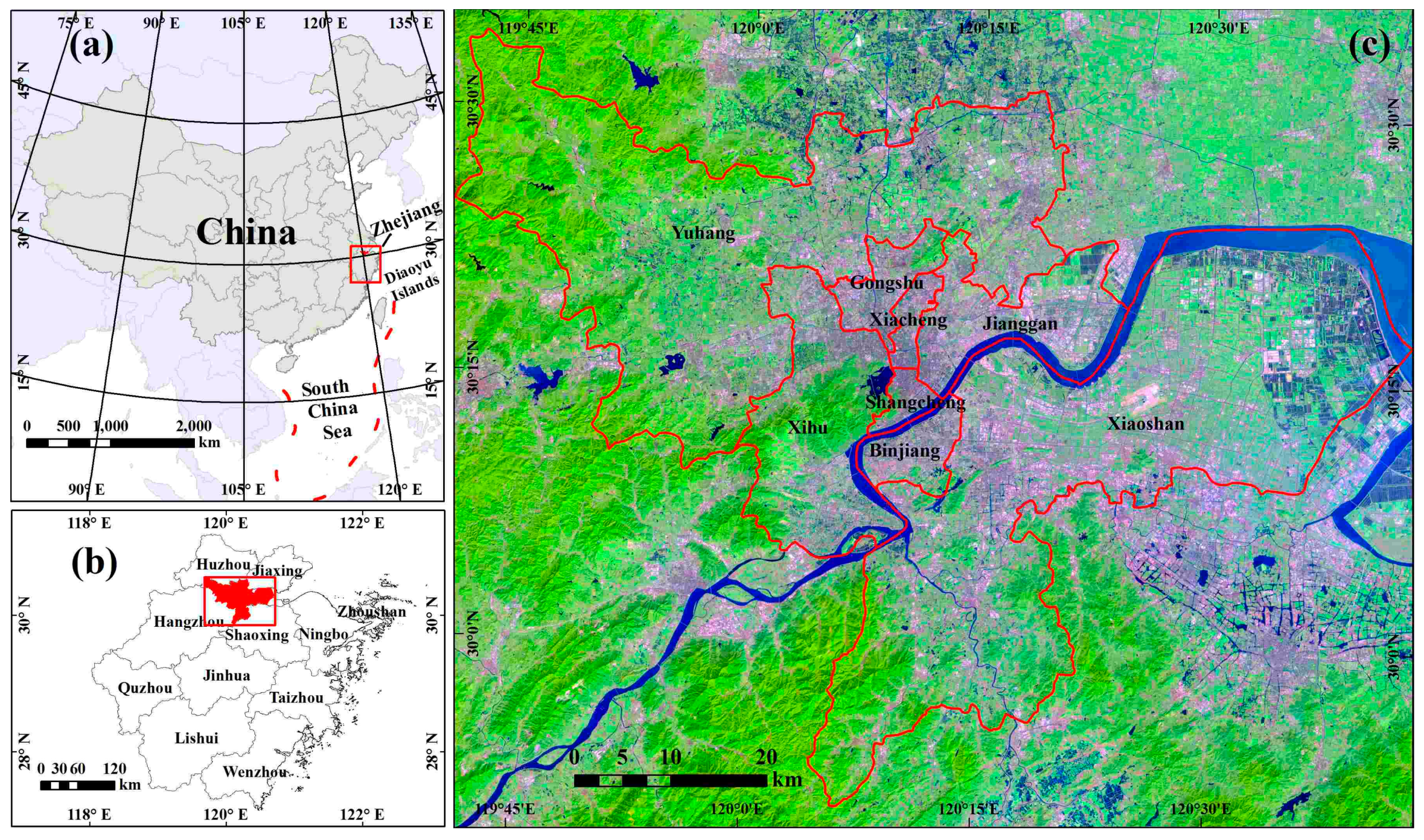
2.1. Study Area

Figure 1 shows the HMA, which is located in the lower reaches of the Qiantang River at latitude from 29°11′N to 30°34′N and longitude from 118°20′E to 120°43′E. The HMA has a classic humid subtropical climate (The Hangzhou Municipal Government, 2016). The annual average temperature is 17.8 °C, and the annual precipitation is approximately 1454 mm. The HMA includes six urban districts and two suburban districts—Shangcheng District, Xiacheng District, Jianggan District, Gongshu District, Xihu District, Binjiang District, Xiaoshan District and Yuhang District—and covers an area of approximately 3068 km2.

2.2. Data Collection and Pre-Processing
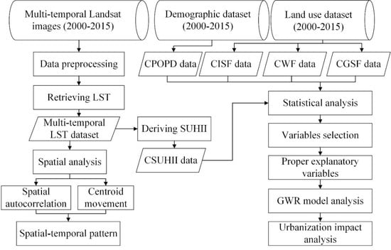
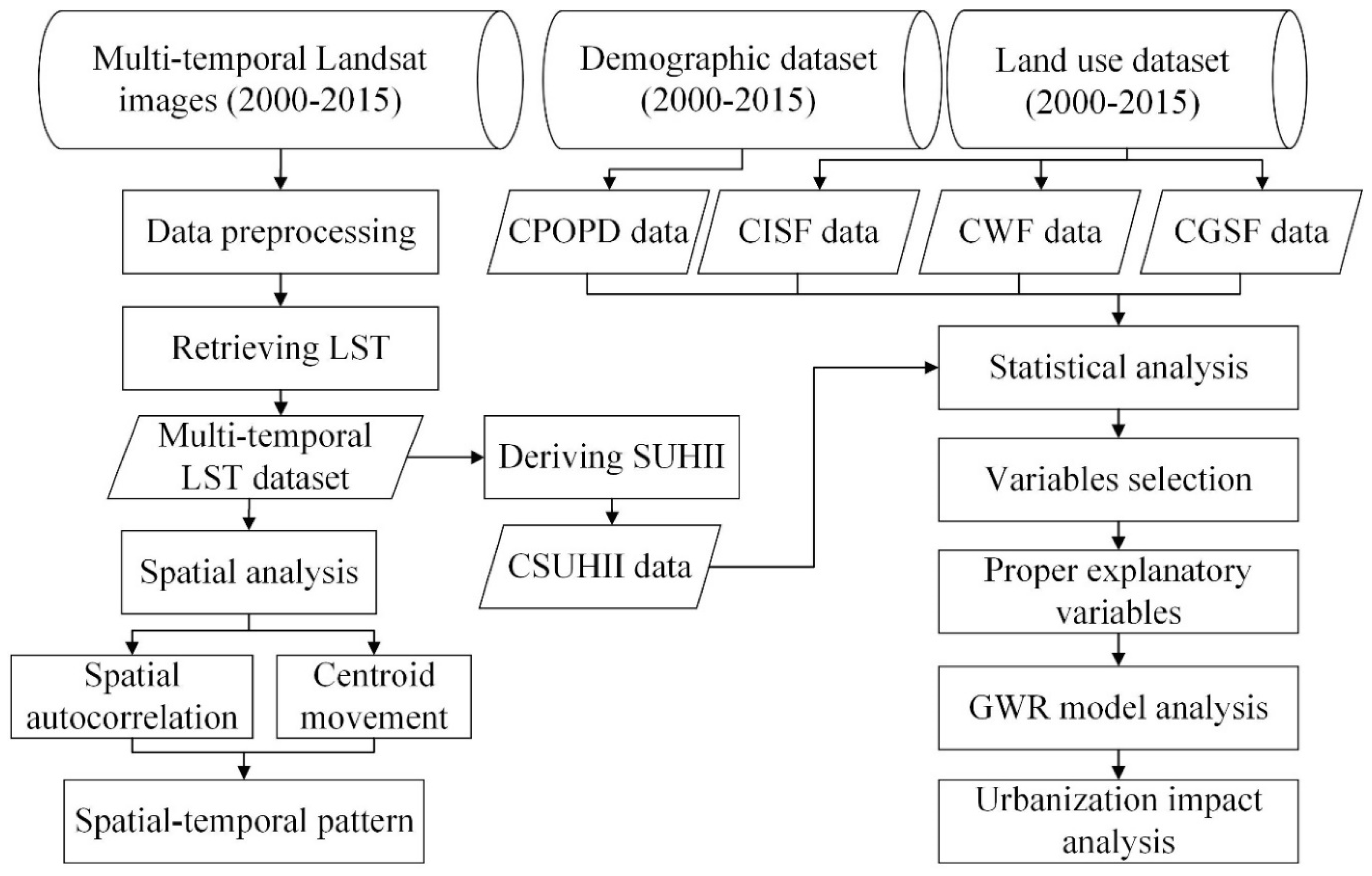
Landsat remote sensing data have been widely used in many case studies on the SUHI effect [11,14,15,17]. Compared with coarse resolution data such as AVHRR and MODIS, Landsat data produce persuasive LST results with higher spatial resolution [24]. Given the SUHI effect together with its adverse effects on environment and human health have been found to be more intense during summer daytime [9], and summer has been identified as the best season in which to examine the thermal environment and urban expansion [14], thus, in our study, the Landsat images that acquired in the summer were utilized to retrieve the LST. Table 1 shows the lists of four collected cloud-free or partly cloudy Landsat-5 TM and Landsat-7 ETM+ images (path 119 and row 39) available from 2000 to 2015 (with a spatial resolution of 30 m), and all Landsat data can be obtained from the Earth Resources Observation and Science Center of USGS (available at http://glovis.usgs.gov/). Images were selected at intervals of five years between 2000 and 2015, following the intervals suggested by a previous study to monitor the urbanization process [25] and the “Five-Year Plan” issued by the Hangzhou municipal government. To minimize the impact of precipitation on the SUHII [26], all images were acquired after at least three days of no precipitation, where the precipitation information was obtained from meteorological observations in the study area. Because the scan line corrector (SLC) of the ETM+ sensor on board Landsat-7 failed permanently, approximately 17% of the SLC-off image data are lost within the study area; therefore, we used a weighted linear regression model to recover the missing pixels in the selected SLC-off images [27]. The gap-filled images contain most of the available information in comparison with SLC-on products and, thus, can be used for our study. The selected images were calibrated by radiometric calibration and atmospheric correction to eliminate the errors caused by the sensor itself and those caused by atmospheric scattering, absorption and reflection. Then, the boundary of the study area was used to clip the calibrated images for subsequent processing.
Table 2 shows the collected auxiliary datasets in this study. Ground-based LST data at 10:00 and 11:00 can evaluate the accuracy of satellite-based LST data in the local time. In addition, other meteorological data (daily mean temperature, daily sunshine duration, daily mean humidity and daily mean wind velocity) for the acquisition dates of the Landsat images can evaluate their influence on the satellite-based LST. The land use dataset was used to extract the impervious surface fraction (ISF), water fraction (WF) and green space fraction (GSF). The demographic dataset was used to estimate the population density (POPD). The land use dataset and demographic dataset were rectified and geo-referenced to the UTM projection.

3. Methodology

Figure 2 illustrates the methodology of this study. First, we estimated the LST from Landsat images. After that, we implemented spatial analysis to depict the spatial-temporal pattern of the SUHI in the HMA during the study period. Spatial autocorrelation analysis via Moran’s I index and hot spot analysis were used to characterize the global and local spatial characteristics of the SUHI. The spatial centroid movement analysis was adopted to illustrate the relationship between urban thermal environment dynamics and urban development in the HMA. Finally, we obtain the SUHI intensity (SUHII) from the estimated LST and conduct statistical analysis using the geographically weighted regression (GWR) model in order to investigate how changes in the potential influencing factors at the different stages of the urbanization process impact the evolution of the SUHI in the HMA. The images pre-processing and LST retrieval were conducted with ENVI 5.3. All spatial analysis and statistical analyses were performed using ArcGIS 10.5, GWR 4 and SPSS 25.

3.1. LST Retrieval

The radiative transfer equation was utilized to estimate LST from the Landsat-5 TM and Landsat-7 ETM+ thermal infrared band (band 6). The LST data were retrieved using the following steps.
First, the top of the atmosphere radiance ( L λ ) was converted to surface-leaving radiance ( L T ) through an atmospheric correction process using Equation (1) [28].
L T = L λ L μ τ ( 1 ε ) L d τ ε
where L μ is the upwelling radiance, L d is the downwelling radiance, τ is the atmospheric transmission and ε is the emissivity of the surface. L μ , L d and τ were calculated using the atmospheric correction parameter calculator online tool (http://atmcorr.gsfc.nasa.gov/), and surface emissivity ( ε ) was calculated using the normalized difference vegetation index (NDVI) thresholds method proposed by [29,30].
Second, land surface temperature ( T s ) was derived using Equation (2) [31]:
T s = K 2 ln ( K 1 L T + 1 )
where K 1 and K 2 are the pre-launch calibration constants. For Landsat-5 TM data, K 1 = 607.76 Wm 2 sr 1 μ m 1 and K 2 = 1260.56 K; for Landsat-7 ETM+ data, K 1 = 666.09 Wm 2 sr 1 μ m 1 and K 2 = 1282.71 K.

3.2. Spatial Analysis of SUHI

Spatial autocorrelation analysis interprets the spatial aggregation pattern of SUHI both on the holistic and local spatial scales. The thermal environment dynamics is closely associated with the urbanization [9], and the changes in spatial aggregations of SUHI can directly reflect the changes of urban spatial pattern at different scales. In this study, Moran’s I [32] was calculated to delineate the global thermal pattern in Equation (3):
I = n i = 1 n j = 1 n ω i j i = 1 n j = 1 n ω i j ( x i x ¯ ) ( x j x ¯ ) i = 1 n ( x i x ¯ ) 2
where x i is the LST value for pixel i, w i , j is the spatial weight between LST pixels i and j, X ¯ is the mean LST and n is the total number of pixels. A positive I indicates the spatial agglomeration of a high or low LST value, whereas negative I indicates the spatial diffusion of a high or low LST value.
In contrast, the hot spot analysis (Getis-Ord G i * ) was adopted to investigate the local spatial clusters within the LST data. The Getis-Ord local statistic was estimated using Equation (4) [33]:
G i * Z s c o r e = j = 1 n ω i , j x j X ¯ j = 1 n ω i , j s [ n j = 1 n ω i , j 2 ( j = 1 n ω i , j ) 2 ] n 1
where G i * Z s c o r e is the Getis-Ord statistics for pixel i, x j is the LST value for pixel j, w i , j is the spatial weight between LST pixels i and j, X ¯ and S are the mean and variance of the LST, respectively, and n is the total number of pixels. A G i * Z s c o r e near zero means no spatial clustering. A higher positive G i * Z s c o r e indicates more intense local clusters of high values (i.e., hot spot), whereas a smaller negative G i * Z s c o r e shows more intense local clusters of low values (i.e., cold spot). The G i * Z s c o r e represents the statistical significance of local clustering for a specified distance (90% significant: >1.65 or <−1.65; 95% significant: >1.96 or <−1.96; 99% significant: >2.58 or <−2.58; 99.9% significant: >3.29 or <−3.29). The 95% or higher confidence level was used in the final statistics of the hot spot analysis. From the statistical results, we manually divided the LST pattern into seven categories: very hot spot, hot spot, warm spot, not statistically significant, cool spot, cold spot and very cold spot.
The spatial centroid has been widely used to explore the urban evolution and changes in the SUHI [34,35]. The centroid of the hot spot and the urban centroid in the HMA for 2000, 2005, 2010 and 2015 were also calculated to depict the relations between the spatial evolution of the SUHI and urbanization in the HMA. The centroid coordinates were calculated according to Equations (5) and (6):
X t = i = 1 n C t i X i i = 1 n C t i
Y t = i = 1 n C t i Y i i = 1 n C t i
where X t and Y t are the mean spatial centroid coordinates of a geographic object; C t i is the area of the i-th of the object and X i and Y i are geometric centroids of the i-th portion.

3.3. Statistical Analysis of SUHII Using GWR

Statistical analysis was used to explore the relations between the SUHI and its influencing factors and to explain how those influencing factors affect the thermal environment dynamics in the HMA. Consequently, we can assess the impact of urbanization on the SUHI by using this method. Although the atmospheric conditions are quite similar among the selected Landsat images, to minimize the synoptic weather effects and the parameters uncertainties in retrieval algorithm, we adopted the SUHII to investigate the evolution of the SUHI rather than the absolute LST value. Because the SUHII can be quantified using the LST difference between urban and rural areas, we subtracted the mean LST of suburban areas from the LST of each pixel within the study area and used the following steps to define urban and suburban areas [36]. First, the urban land polygons in land use data were used to delineate the urban border. The land within the border was defined as urban area (excluding water pixels). After that, a buffer zone surrounding the urban area was created to have the same size as the urban area (excluding water pixels, as well as all the rural pixels having an altitude greater than the mean urban altitude). Finally, it was defined as the suburban area for further analysis.
In our study, the SUHII of HMA was divided into three different stages (i.e., 2000–2005, 2005–2010 and 2010–2015), and CSUHII were used as the dependent variable. The SUHII correlates closely with urban population density, impervious surface, water body and vegetation coverage. By referring to previous studies [15,37], the population in the analytical grid unit was used to quantify the POPD, the percentage of construction land area in the analytical grid unit was utilized to characterize the ISF, the percentage of water bodies area in the analytical grid unit was adopted to measure the WF and the percentage of cultivated land, forest and grass land areas in the analytical grid unit was implemented to represent the GSF. The changes in these four factors were utilized as potential explanatory variables, including CPOPD, CISF, CWF and CGSF. The dependent variable and these explanatory variables were calculated at the analytical grid unit level. To reduce the amount of data for the statistical analysis, the grid size could not be too small for the regional scale of this study. The Landsat data products were resampled by USGS to 30 m, and the side length of any grid should be an integer multiple of 30 m. The analytical grid unit sizes should match the pixel size of the demographic data. Accordingly, in order to facilitate the subsequent statistical analysis, all of the data for the dependent variable and explanatory variables were calculated with a grid size of 1200 m × 1200 m. We extracted mean values of CPOPD, CISF, CWF, CGSF and CSUHII from each analytical grid unit. After that, we implemented the correlation analysis and ordinary least square (OLS) on them to eliminate the multicollinearity problem and meanwhile test the significance of these initial variables for inputting into the GWR model.
The GWR model is a local form of a linear regression used to model spatially varying relationships. This model accounts for spatial autocorrelation and spatial non-stationary issues and behaves better than OLS [38]. In this paper, the GWR model investigates the correlations between CSUHII effect and the changes in the associated driving forces in the HMA, as:
y i = β i 0 + k = 1 p β i k x i k + ϵ i ; i = 1 , n ; k = 1 p
where y i represents the value of the dependent variable (i.e., CSUHII) for pixel i; x i k is the k-th independent variable for grid unit i; β i k is the local regression coefficient for the k-th independent variable in grid unit i; β i 0 is the intercept parameter for pixel i and ϵ i is the random disturbance for grid unit i. The performance of GWR model correlates with the kernel type (i.e., fixed and adaptive) and bandwidth method (e.g., Akaike Information Criterion, Cross Validation and bandwidth-parameter). We implemented the adaptive bi-square kernel function and the Akaike information criterion [39] in the regression analysis. Moreover, we employed the solution proposed by da Silva and Fotheringham [40] to solve the problem of multiple testing in GWR model.

4. Results

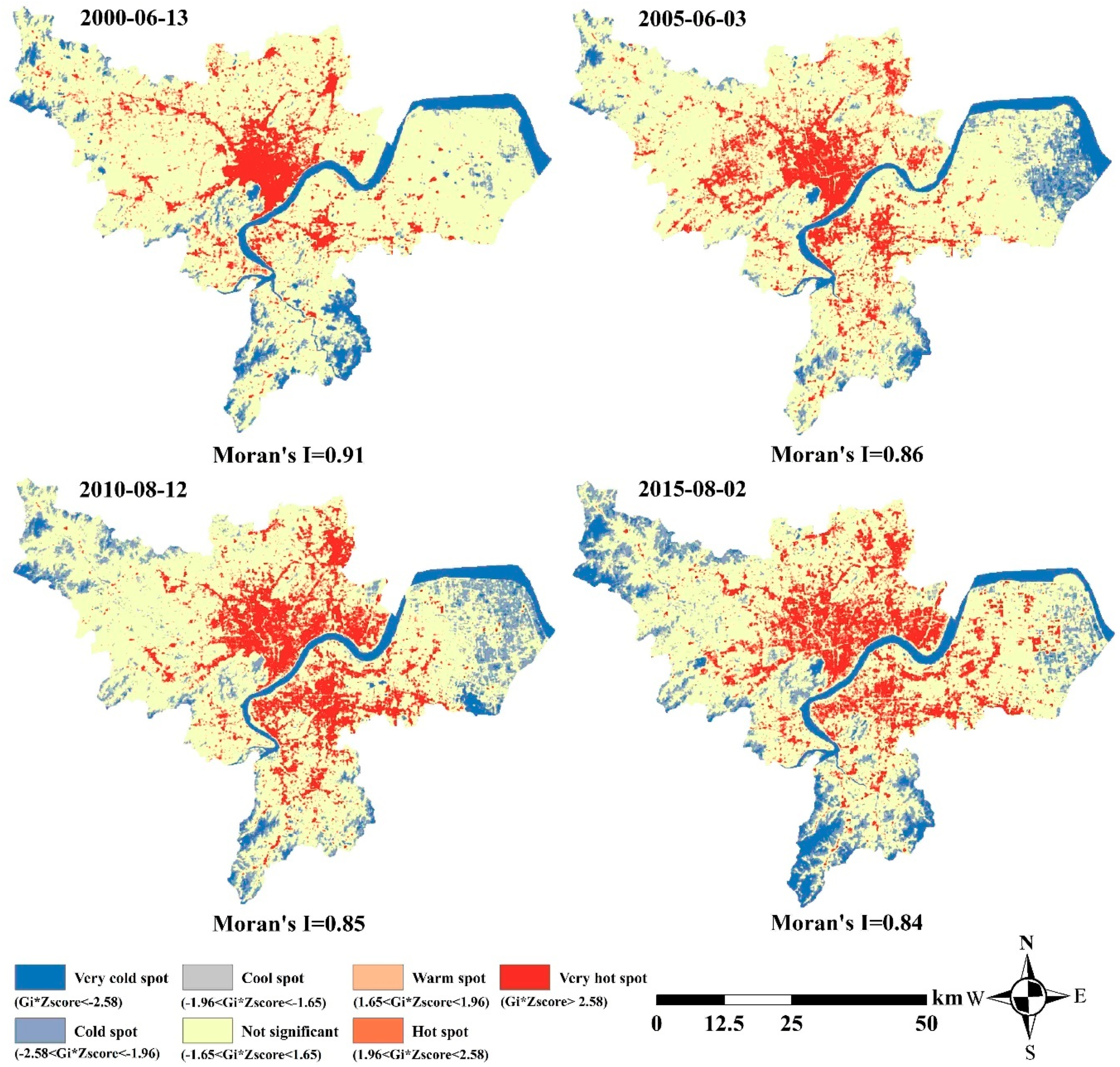
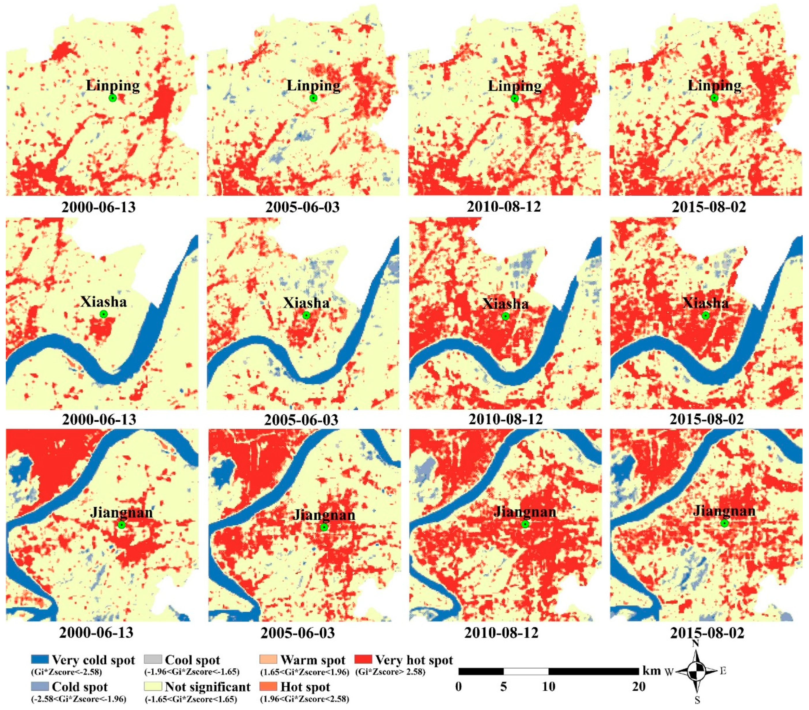
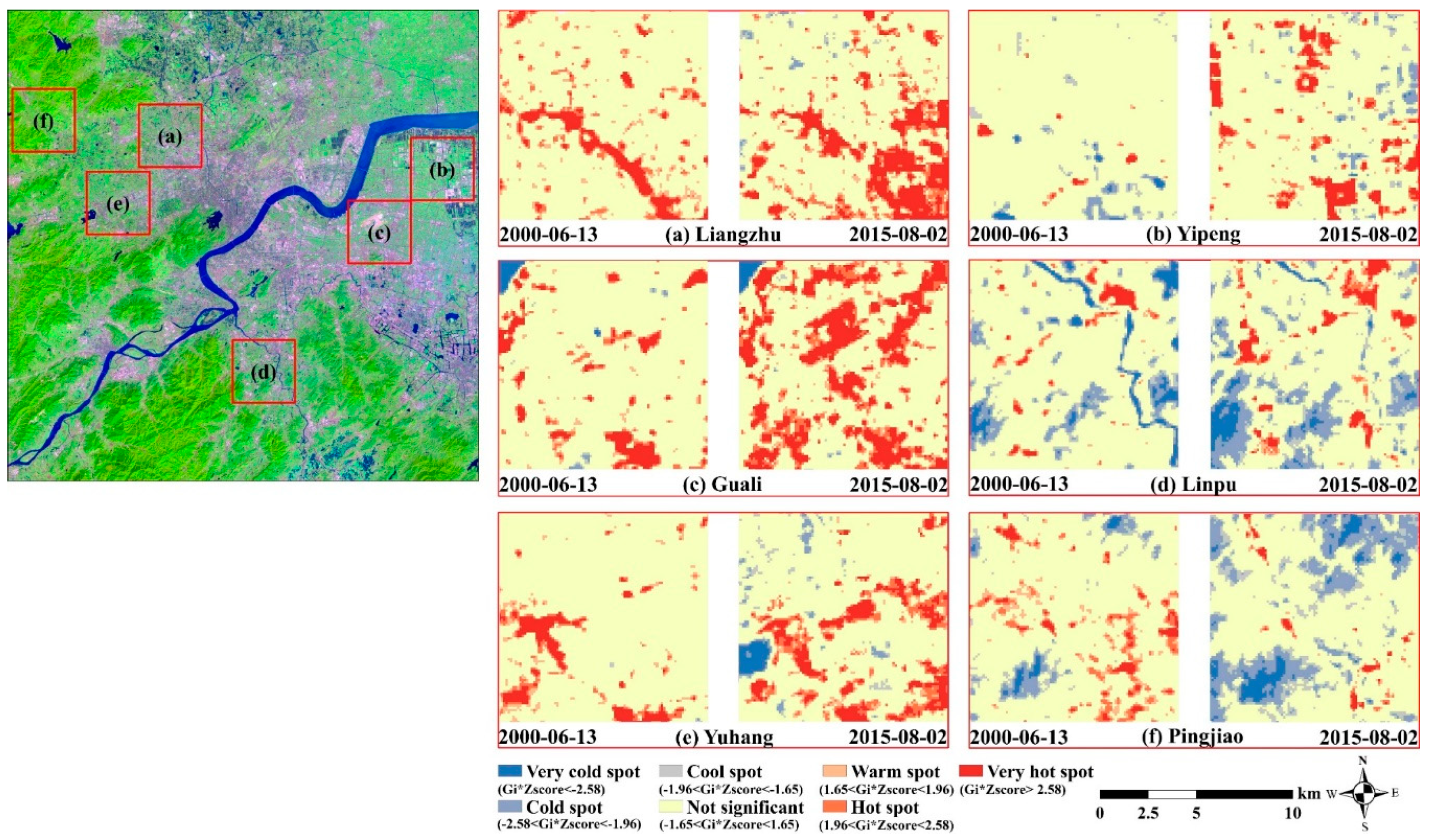
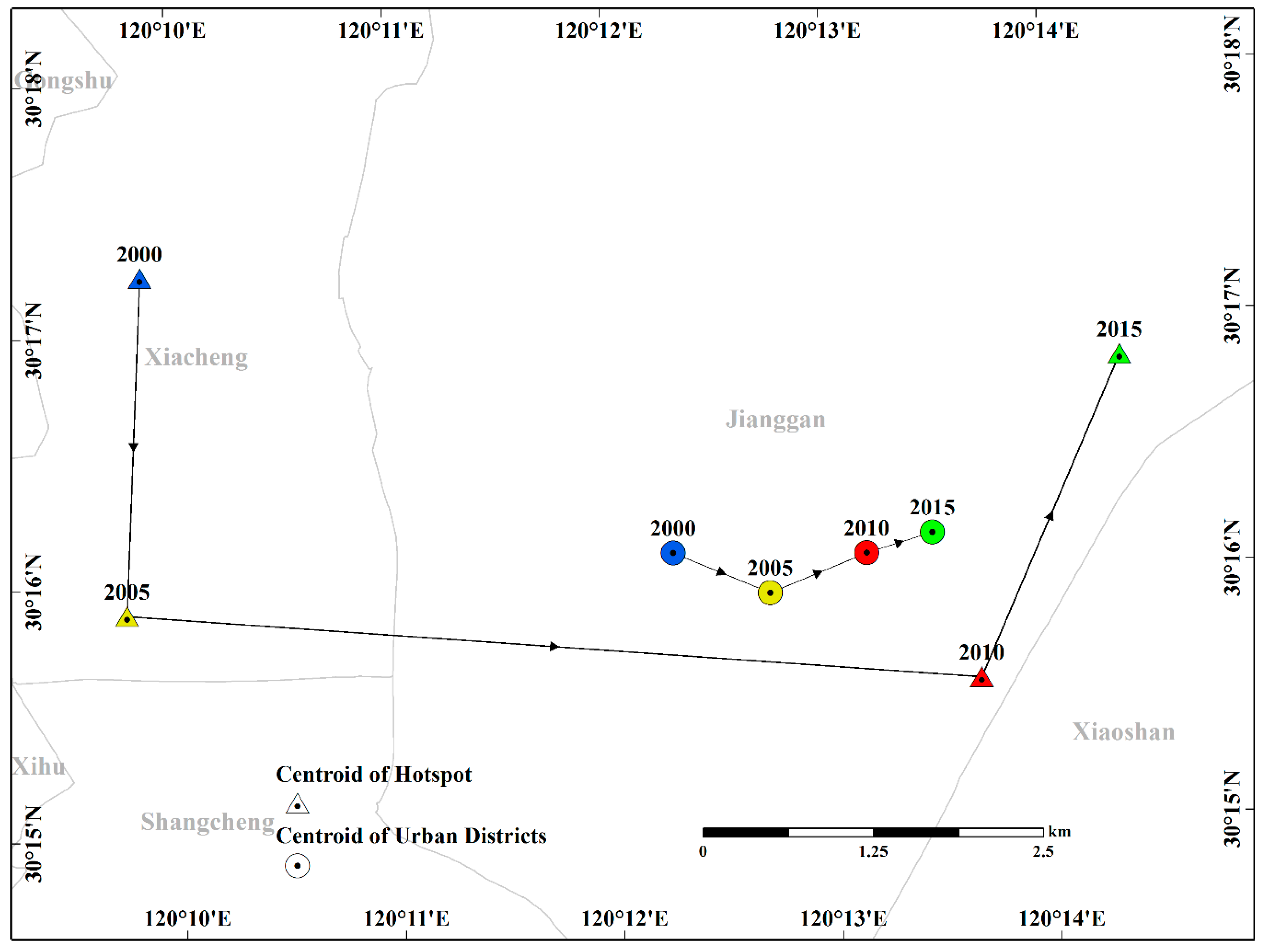
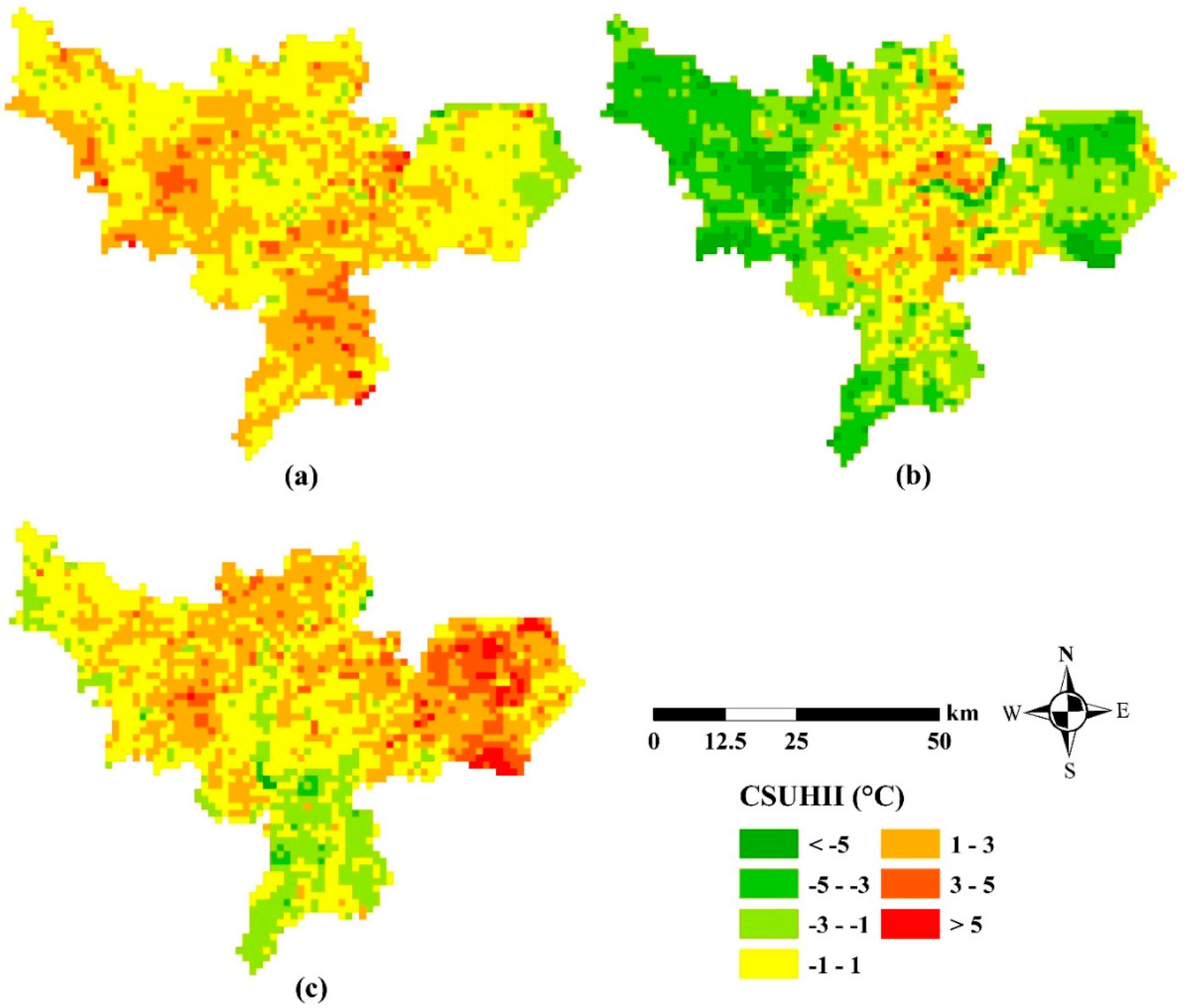
4.1. Spatiotemporal Patterns of SUHI

We estimated the LST from Landsat data and compared ground-based LST data with 28 satellite-based LST sample points at the same locations. The determination coefficient between them was 0.86. In addition, the root mean square error (RMSE) and standard deviation (STD) of the satellite-based LST were 1.95 °C and 4.31 °C, respectively. According to Table 1, the average wind speed was less than 2.0 m/s and the daily precipitation of all days was 0 mm. These results further confirm the acceptability of the satellite-based LST for further analysis.
Figure 3 describes the spatial pattern of the SUHI in the HMA throughout the study period. From 2000 to 2015, hot and very hot spot areas expanded outwards along with the urbanization process in the HMA. The evolution of hot spots in the HMA changes from a monocentric pattern to a polycentric pattern. The value of Moran’s I is continuously decreasing during 2000–2015, indicating that the sparse aggregation pattern and the thermal environment of the HMA has become more homogenous. These changes were highly consistent with urban sprawl of the HMA throughout the study period, they mirrored the intensive development of three satellite towns. In addition, in the HMA, the hot and very hot spot areas exist in the urban centre, along main roads and industrial zones, whereas the cold and very cold spot areas are present in vegetated surfaces, Qiantang River, Xixi National Wetland Park and West Lake. This finding indicates that green space and water bodies play an important role in alleviating the SUHI effect. Some insignificant areas, such as the cultivated lands on the outskirts of the urban area, became hot spots during 2000–2015, and the area proportions for the hot and very hot spot areas increased (from 11.5% in 2000 to 18.3% in 2015) during the entire study period.
Moreover, we analysed the spatial pattern of the SUHI in the three satellite towns of Linping, Xiasha and Jiangnan. The first row of Figure 4 illustrates the SUHI evolution of Linping town. The concentrated hot and very hot spot areas moved to the outskirts during the study period. Linping town is a traffic hub in the HMA, and the agglomeration of population, industry and transportation infrastructure significantly changed its thermal environment. The second row of Figure 4 shows the SUHI evolution of Xiasha town. The rapid aggregation of college students, high-quality talents and skilled workers caused some areas to change from insignificant and warm spots to hot and very hot spots. The third row of Figure 4 shows the SUHI evolution of Jiangnan town, which indicated a similar change trend as that of Linping and Xiasha during 2000–2010. However, the Binjiang High-tech Development Zone in the town attracted a large number of relatively light industries during 2010–2015 and a number of high-tech enterprises are distributed in well-planned neighbourhoods. These results indicate that the SUHI effect was alleviated in 2015 relative to 2010. Moreover, Figure 5 shows the SUHI evolution of several key town groups in the HMA during 2000–2015. The Liangzhu, Yipeng, Guali and Yuhang town groups in the HMA have an increasingly severe SUHI along with their rapid urbanization process. The town groups of Linpu and Pingjiao are located in the fringe of the study area and have relatively high elevation and abundant vegetation coverage, and urban development has little effect on these regions. Consequently, their cold and very cold spot areas show an increased trend.
Furthermore, Figure 6 shows the centroid trajectories of hot and very hot spot areas and the urban area in HMA during 2000–2015. The centroid of hot and very hot spot areas was in the left of the urban centroid in 2000 and moved eastwards and northwards in 2005 and 2010, respectively. The centroid of hot and very hot spot areas moved eastwards during the entire study period, coinciding with the moving direction of the urban centroid. The movement of the urban centroid was related to the development strategies implemented in the HMA: “Moving from the West Lake Times towards Qiantang River Times.” The economy and society in the east of the HMA and the south bank of the Qiantang River have achieved higher growth rates. To the south is Binjiang District, where a state-level economic and technological development zone is located. To the east is Jianggan District, where Xiasha university town and Jiubao industrial park are located. The rapid development in these areas resulted in more high-LST clusters, making the centroid of the hot spots move eastwards in general.

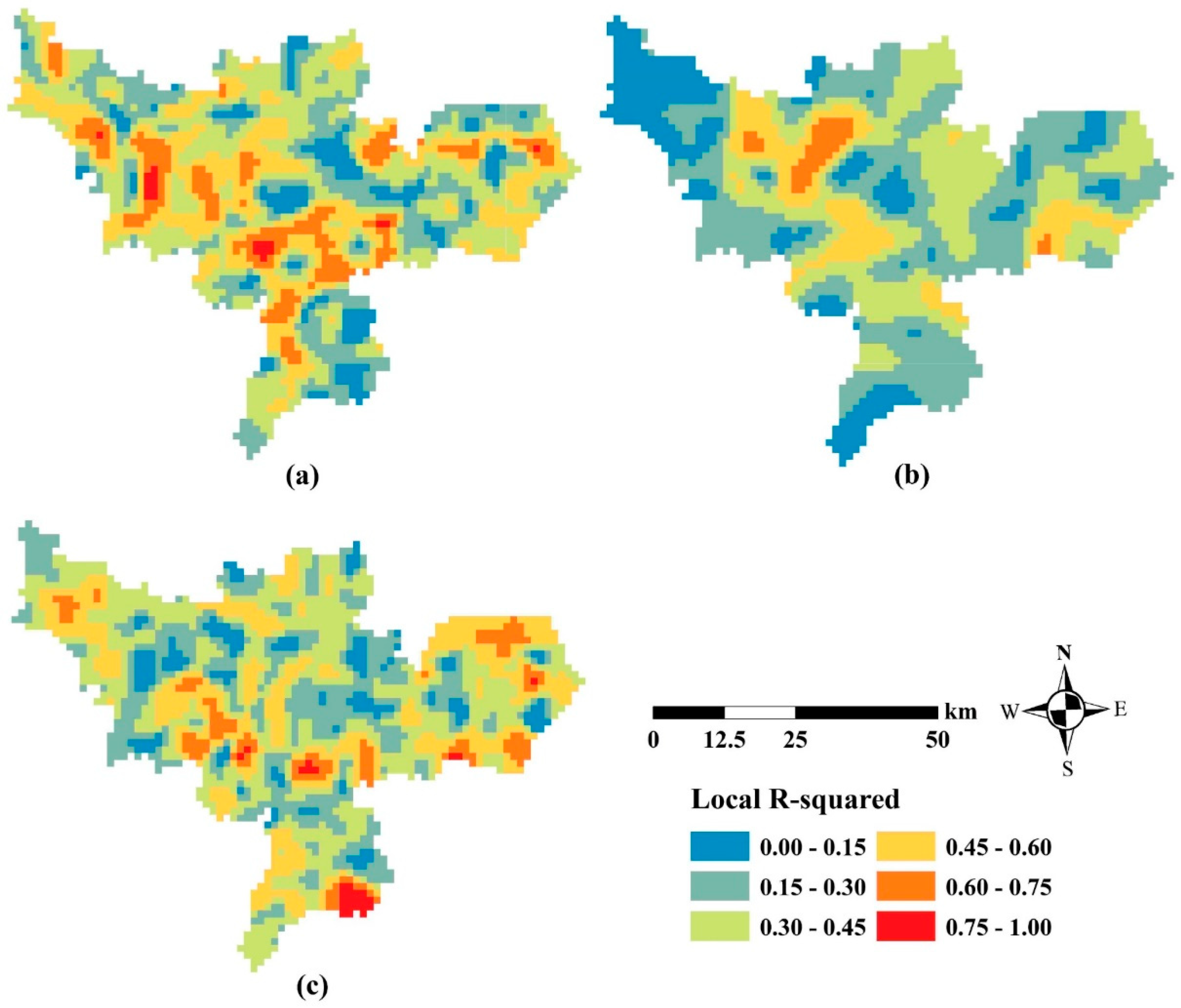
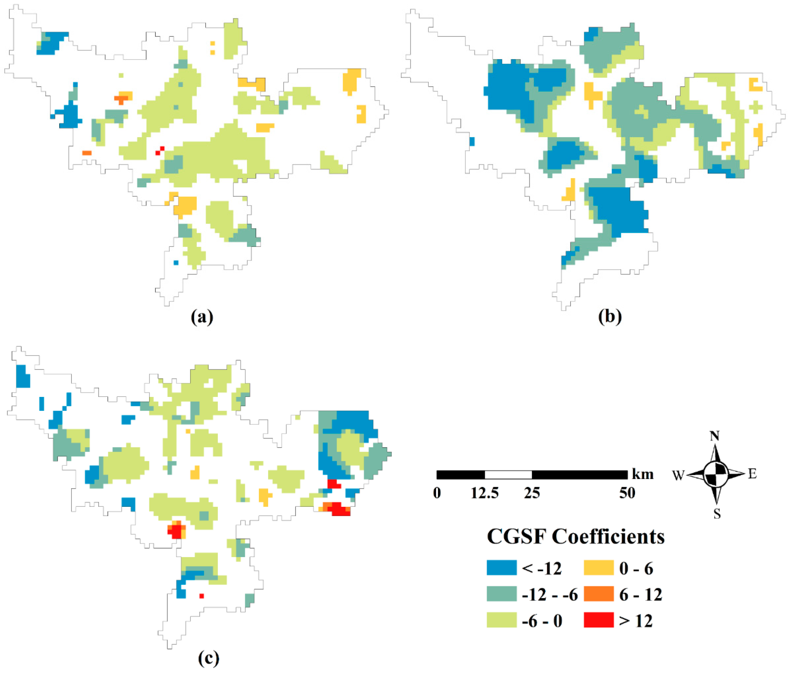
4.2. Statistical Analysis

During the study period, the population density of the HMA increased from 1216 people per km2 in 2000 to 1519 people per km2 in 2015 (The Hangzhou Statistic Bureau, available at http://tjj.hangzhou.gov.cn/). The rapid population growth brings remarkable landscape changes. Table 3 shows the changes in area proportions of major landscapes in the HMA. Between 2000 and 2015, the area proportions of impervious surface increased by 12.0%, approximately equivalent to a total decrease of water bodies and green space. However, the decrease in cultivated land accounts for a large amount of the decrease in green space (i.e., decreased by 9.4%). These changes indicate that the study area has undergone rapid urbanization during the past decades.
Figure 7 shows the CSUHII in the HMA during the different stages. During 2000–2005, some exurban areas (i.e., Liangzhu, Yuhang and Linpu) and suburban areas (i.e., Linping, Xiasha, Jiangnan) were subjected to an increase in SUHII. During 2005–2010, exurban areas experienced a reduction in SUHII, whereas suburban areas subjected to urban expansion still remained on an upward trend in SUHII. During 2010–2015, Linping and Xiasha, as well as parts of the exurban area (i.e., Liangzhu, Yipeng, Guali and Yuhang) showed an increased trend in SUHII. In summary, these changes indicate that the suburban areas and parts of the exurban areas in the HMA have been influenced by the enhanced the SUHI effect between 2000 and 2015.
Prior to conducting the regression analysis, a correlation analysis was conducted among the selected explanatory variables. The correlation analysis results indicate that CPOPD were highly correlated with CISF. In addition, CWF did not pass the OLS significance test. Thus, we only preserved CPOPD and CGSF as explanatory variables to construct the GWR model. Figure 8 shows the local R2 values of this GWR model. The R2 varies significantly over the HMA, and a high R2 indicates that selected variables can better explain CSUHII. The suburban (i.e., Linping, Xiasha and Jiangnan) and exurban areas (i.e., Liangzhu, Yipeng, Linpu and Yuhang) always have better fitting results than the urban area during the three stages (i.e., 2000–2005, 2005–2010, 2010–2015). It indicates that changes in the population density and greenspace in these areas strongly impact on the changes in SUHII, accordingly, we just need to focus on these two factors dynamics in above mentioned areas when mitigating SUHI effect. Table 4 shows the results and diagnostics of the statistical analysis in the GWR model. The adjusted R2, Akaike Information Criterion (AICC) and Moran’s I index indicate that the GWR model yielded reliable results. The coefficients show that an increase in population density can increase the SUHII, whereas an increase in green space can reduce the SUHII. Specifically, the larger coefficient in CGSF indicates that the increase in green space is most important to reducing the SUHII during the different stages of the urbanization process in the HMA.
In order to further investigate the impacts from CPOPD and CGSF in the evolution of SUHII in the HMA, we only show local parameter estimates that are statistically significant according to the corrected t-values in each stage [41,42] in Figure 9 and Figure 10. The mean coefficients of CPOPD during the three stages reaches up to 0.0003, 0.0005 and 0.0030, indicating the intensifying effect from growing population density on increasing SUHII during the three stages. Local relationships between CPOPD and CSUHII are highly significant in some suburban and exurban areas of the HMA. For instance, the CPOPD has a statistically significant negative influence on the CSUHII in the northwest of Yuhang District, the southwest of Xiaoshan District and part of the central districts during 2000–2015. This result indicates that these areas experienced population outmigration during this period. In contrast, the CPOPD has a statistically significant high positive effect on some exurban areas (i.e., Yipeng, Linpu, Yuhang and Pingjiao) during 2000–2015, explaining that significant population migration occurred during the study period.
Figure 10 describes local parameter estimates for the relationship between CGSF and CSUHII. The mean CGSF coefficients during the 16 years decrease from −1.6178 in stage one (i.e., 2000–2005) to –11.7569 in stage three (i.e., 2010–2015), indicating that an increase in green space can have a significant mitigating effect on the SUHII at different stages of the urbanization process in the HMA. The majority of the local estimates are statistically significant negative during the three stages, however the local relationships between CGSF and CSUHII also showed a statistically significant positive in some exurban and suburban areas, coinciding with the urban expansion and the cultivated land loss within the identical region of same period.

5. Discussion

5.1. Relationship Between Urban Development and Spatial Pattern of SUHI

Since the 2000s, the “Tenth Five-Year Plan” issued by the Hangzhou municipal government has communicated that the Hangzhou will be an economically strong, cultural and international tourism city. Accordingly, the urban area is oriented as an agglomeration for tourism, the software industry, modern services and the urban industry, whereas the suburban and exurban areas house industries transferred and universities relocated from the urban area. Therefore, the spatial-temporal pattern of the SUHI with respect to political and socio-economic conditions in the HMA during the 16 years can be explained as follows.
In 2001, administrative boundaries between Yuhang District, Xiaoshan District and the former city were readjusted and merged to formulate the new HMA. Subsequently, the government-oriented polices of industrial restricting and college relocations were developed and implemented. As a result, many traditional industrial polluters moved to suburban or exurban industrial parks (e.g., Hangzhou Iron & Steel Group Company of China) and several universities and colleges (e.g., China Jiliang University, Hangzhou Normal University and Zhejiang Gongshang University) moved to college parks near the industrial parks. Accordingly, the eastern part of Yuhang District and Jianggan District, and Linping and Xiasha satellite towns attracted millions of intra-provincial and inter-provincial migrants. Meanwhile, rapid aggregation of the population and high-tech industries in the Binjiang High-tech Development Zone and Xiaoshan Economic Development Zone enhanced the development of Jiangnan satellite town. As the strategies of frog-leaping development along the Qiantang River gradually advanced in depth, construction of the transportation infrastructure (e.g., Zhijiang Bridge, Jiubao Bridge) has been accelerated, the linkage between the urban area and new towns along the Qiantang River banks is closer and the polycentric development pattern of the HMA became increasingly mature. In summary, rapid urban development along the Qiantang River and the eastern part of HMA has resulted in the eastward and southward expansion of the urban area. Accordingly, during the study period, the hot spot areas of the HMA became more scattered, its spatial distribution changed from a monocentric to a polycentric pattern, and its centroid moved eastwards—this outcome is highly consistent with the urban centroid movement direction. These changes mirrored the city’s intensive development of three satellite towns during the study period.

5.2. Implications for Mitigating SUHI Effect

The hot spot analysis results showed an increase in high-LST clusters and a decrease in the areas which are not statistically significant. Thus, to control the formation of the SUHI in not significant areas on the outskirts of urban area, urban planners and policymakers should pay much attention to the development in these regions. In addition, the hot and very hot spot areas exist in the impervious surface along the Qiantang River, whereas the significant cold spot areas are present in the vegetation surfaces, rivers and lakes. Therefore, the green space and water bodies play a key role in mitigating the SUHI effects through evapotranspiration. However, given scarce land resources, merely increasing the green space and water bodies in the aforementioned hot and very hot spot areas to offset the SUHI effects is difficult. Thus, taking other proper mitigation measures is necessary, such as adopting green roofs and cool pavements [43]. Moreover, when mitigating the SUHI effect in hot and very hot spot areas, considering the influences of the background temperature [44] and meteorological characteristics [45] is essential. For instance, green space is not sufficient to mitigate the SUHI effects in high density built-up areas given its small fraction, making it important to rationally restrict the development scale and avoid fragmentation of vegetation covers in hot and very hot spot areas. Although the wind can transport much more cool sources into dense urban areas and discharge excess urban heat, we can control the height and density of buildings in hot and very hot spot areas to construct urban ventilation corridors to mitigate the SUHI effects.
The statistical analysis results indicated that the rapid population growth of the HMA has brought remarkable changes in land use and transformed cultivated lands into impervious surfaces and that green space reduced in the suburban and exurban areas, coinciding with these areas continuing to experience an upward trend in the SUHII. The results also showed that increasing green space can significantly reduce the SUHII, whereas increasing population density can elevate the SUHII to a certain extent. However, green space has a stronger effect on modifying the SUHII than population density at the different stages of the urbanization process, indicating that accommodating population growth in suburban and exurban areas without reducing green space is important for mitigating the SUHI effect. Therefore, to effectively alleviate the SUHI effect, blind urban expansion must be avoided and protecting cultivated lands in suburbs and exurbs is urgently needed, as is improving the utilization efficiency of construction land by encouraging the migrating population to live within the existing built-up regions.

5.3. Limitations of This Study

Our study has investigated thermal environment dynamics of the HMA in the context of the urbanization process from 2000 to 2015. However, given poor temporal resolution and the influence of cloud cover, we used only 4 Landsat scenes that were acquired in the summer to explore inter-annual thermal trends. The UHI effect correlates closely with the weekly cycle of human activities [46,47,48]. The implemented 4 Landsat images have different collection days during one week. That might bring about divergent anthropogenic influence in the UHI effects and degrades the integrity of our conclusion obtained. On the other hand, the 4 Landsat images were collected in different synoptic and weather conditions (e.g., cloud cover and wind speed). The inconsistency of synoptic and weather conditions has been proven to negatively affect the comparability of UHI effects and hot spots in different days [49,50,51], which also might limit the rigorousness of above analysis result. In the future, we will carefully analyse the impacts from both the weekly cycle of human activities and the synoptic and weather conditions, and implement more Landsat-LST time series that are derived from multi-temporal and multi-sensor fusion methods [9,52,53] to continue improving our study. Moreover, we will try to utilize the local climate zones for the SUHII calculations to mitigate the effect of the differences in vegetation phenology [54] and obtain more comprehensive results. Additionally, to capture the complexity of the influencing factors in the SUHI, we will consider urban morphology (e.g., building height, sky view factor) as an influential factor [18] and involve other advanced models (e.g., artificial neural network and decision tree) in order to explore the nonlinear relationship between the influencing factors and the SUHI in urban areas.

6. Conclusions

This paper investigated the spatiotemporal evolution of the SUHI in the HMA from 2000 to 2015 and explored how the main influencing factors during the three stages of the urbanization process (i.e., 2000–2005, 2005–2010, 2010–2015) affected changes in the SUHI. This study has significant implications for sustainable urban planning in the HMA.
Hot spot analysis is an effective method for depicting the spatial pattern of a SUHI over time, which is consistent with exiting study [18]. In general, hot and very hot spot areas increased from 387 km2 in 2000 to 615 km2 in 2015, the spatial distribution changed from a monocentric to a polycentric pattern, and the centroid moved towards the east; this outcome was highly consistent with urban expansion throughout the study period. These changes mirrored the intensive development of three satellite towns.
The statistical analysis results showed that changes in SUHII depend on the geographical context and that the effect should be modelled locally, coinciding with an existing study [19]. We used a local-based model to assess the relationship between influencing factor dynamics and changes in SUHII at different stages of the urbanization process. Overall, an increasing in population density had a lasting effect in elevating the SUHII (mean coefficients of CPOPD increase from 0.0003 to 0.0030), whereas an increase in green space had a significant effect in mitigating the SUHII (mean coefficients of CGSF decreased from −1.6178 to −11.7569). However, green space has a stronger effect on modifying the SUHII than population density at the different stages of the urbanization process, indicating that accommodating population growth in suburban and exurban areas without reducing the green space is important for mitigating the SUHI effect.
According to the aforementioned analysis results, urban planners and policymakers should pay significant attention to the insignificant areas on the outskirts of urban areas and must consider optimizing the spatial pattern of landscapes in hot and very hot spot areas. For example, schemes include clustering vegetation, constructing urban ventilation corridors and adopting green roofs and cool pavements. Moreover, avoiding blind urban expansion and protecting cultivated lands in the suburbs and exurbs of the HMA, and improving the utilization efficiency of construction land by encouraging the migration population to live within the existing built-up regions should be considered in urban planning for the sustainable development of the HMA.

Author Contributions

F.L. and W.S. analyzed the data, performed the experiments and wrote the draft of the manuscript; Q.W. helped to redesign the methodology, review and revise the manuscript; G.Y. designed the framework of this study, gave comments and significantly revised the manuscript.

Funding

This research was funded in part by the National Natural Science Foundation under Grant 41671342 and Grant U1609203, in part by the Natural Science Foundation of Zhejiang Province under Grant LR19D010001 and Grant LQ18D010001, in part by the Ningbo Natural Science Foundation under Grant 2017A610294, and in part by the K. C. Wong Magna Fund from Ningbo University.

Acknowledgments

The authors would like to thank the editor and referees for their suggestions and commnets that helped to improve the manuscript.

Conflicts of Interest

The authors declare no conflict of interest.

References

  1. Ayanlade, A. Seasonality in the daytime and night-time intensity of land surface temperature in a tropical city area. Sci. Total Environ. 2016, 557, 415–424. [Google Scholar] [CrossRef] [PubMed]
  2. Li, Z.-L.; Tang, B.-H.; Wu, H.; Ren, H.; Yan, G.; Wan, Z.; Trigo, I.F.; Sobrino, J.A. Satellite-derived land surface temperature: Current status and perspectives. Remote Sens. Environ. 2013, 131, 14–37. [Google Scholar] [CrossRef] [Green Version]
  3. Sun, W.; Du, B.; Xiong, S. Quantifying Sub-Pixel Surface Water Coverage in Urban Environments Using Low-Albedo Fraction from Landsat Imagery. Remote Sens. 2017, 9, 428. [Google Scholar] [CrossRef]
  4. Voogt, J.A.; Oke, T.R. Thermal remote sensing of urban climates. Remote Sens. Environ. 2003, 86, 370–384. [Google Scholar] [CrossRef]
  5. Gabriel, K.M.A.; Endlicher, W.R. Urban and rural mortality rates during heat waves in Berlin and Brandenburg, Germany. Environ. Pollut. 2011, 159, 2044–2050. [Google Scholar] [CrossRef]
  6. Sarrat, C.; Lemonsu, A.; Masson, V.; Guedalia, D. Impact of urban heat island on regional atmospheric pollution. Atmos. Environ. 2006, 40, 1743–1758. [Google Scholar] [CrossRef]
  7. Jiang, M.; Sun, W.; Yang, G.; Zhang, D. Modelling Seasonal GWR of Daily PM2.5 with Proper Auxiliary Variables for the Yangtze River Delta. Remote Sens. 2017, 9, 346. [Google Scholar] [CrossRef]
  8. Fu, P.; Weng, Q. A time series analysis of urbanization induced land use and land cover change and its impact on land surface temperature with Landsat imagery. Remote Sens. Environ. 2016, 175, 205–214. [Google Scholar] [CrossRef]
  9. Zhou, D.; Xiao, J.; Bonafoni, S.; Berger, C.; Deilami, K.; Zhou, Y.; Frolking, S.; Yao, R.; Qiao, Z.; Sobrino, A.J. Satellite Remote Sensing of Surface Urban Heat Islands: Progress, Challenges, and Perspectives. Remote Sens. 2019, 11, 48. [Google Scholar] [CrossRef]
  10. Eludoyin, O.M.; Adelekan, I.O.; Webster, R.; Eludoyin, A.O. Air temperature, relative humidity, climate regionalization and thermal comfort of Nigeria. Int. J. Climatol. 2014, 34, 2000–2018. [Google Scholar] [CrossRef]
  11. Jiang, Y.; Fu, P.; Weng, Q. Assessing the Impacts of Urbanization-Associated Land Use/Cover Change on Land Surface Temperature and Surface Moisture: A Case Study in the Midwestern United States. Remote Sens. 2015, 7, 4880–4898. [Google Scholar] [CrossRef] [Green Version]
  12. Alavipanah, S.; Wegmann, M.; Qureshi, S.; Weng, Q.; Koellner, T. The Role of Vegetation in Mitigating Urban Land Surface Temperatures: A Case Study of Munich, Germany during the Warm Season. Sustainability 2015, 7, 4689–4706. [Google Scholar] [CrossRef] [Green Version]
  13. Haashemi, S.; Weng, Q.; Darvishi, A.; Alavipanah, K.S. Seasonal Variations of the Surface Urban Heat Island in a Semi-Arid City. Remote Sens. 2016, 8, 352. [Google Scholar] [CrossRef]
  14. Peng, J.; Xie, P.; Liu, Y.; Ma, J. Urban thermal environment dynamics and associated landscape pattern factors: A case study in the Beijing metropolitan region. Remote Sens. Environ. 2016, 173, 145–155. [Google Scholar] [CrossRef]
  15. Estoque, R.C.; Murayama, Y. Monitoring surface urban heat island formation in a tropical mountain city using Landsat data (1987–2015). ISPRS J. Photogramm. Remote Sens. 2017, 133, 18–29. [Google Scholar] [CrossRef]
  16. Du, H.; Wang, D.; Wang, Y.; Zhao, X.; Qin, F.; Jiang, H.; Cai, Y. Influences of land cover types, meteorological conditions, anthropogenic heat and urban area on surface urban heat island in the Yangtze River Delta Urban Agglomeration. Sci. Total Environ. 2016, 571, 461–470. [Google Scholar] [CrossRef]
  17. Song, J.; Du, S.; Feng, X.; Guo, L. The relationships between landscape compositions and land surface temperature: Quantifying their resolution sensitivity with spatial regression models. Landsc. Urban Plan. 2014, 123, 145–157. [Google Scholar] [CrossRef]
  18. Tran, D.X.; Pla, F.; Latorre-Carmona, P.; Myint, S.W.; Caetano, M.; Kieu, H.V. Characterizing the relationship between land use land cover change and land surface temperature. ISPRS J. Photogramm. Remote Sens. 2017, 124, 119–132. [Google Scholar] [CrossRef] [Green Version]
  19. Deilami, K.; Kamruzzaman, M. Modelling the urban heat island effect of smart growth policy scenarios in Brisbane. Land Use Policy 2017, 64, 38–55. [Google Scholar] [CrossRef]
  20. Deilami, K.; Kamruzzaman, M.; Hayes, F.J. Correlation or Causality between Land Cover Patterns and the Urban Heat Island Effect? Evidence from Brisbane, Australia. Remote Sens. 2016, 8, 716. [Google Scholar] [CrossRef]
  21. Chow, D.H.C.; Darkwa, J.; Shen, T. Simulating the influence of microclimatic design on mitigating the Urban Heat Island effect in the Hangzhou Metropolitan Area of China. Int. J. Low-Carbon Technol. 2013, 11, 130–139. [Google Scholar]
  22. Sheng, L.; Tang, X.; You, H.; Gu, Q.; Hu, H. Comparison of the urban heat island intensity quantified by using air temperature and Landsat land surface temperature in Hangzhou, China. Ecol. Indic. 2017, 72, 738–746. [Google Scholar] [CrossRef]
  23. Sheng, L.; Lu, D.; Huang, J. Impacts of land-cover types on an urban heat island in Hangzhou, China. Int. J. Remote Sens. 2015, 36, 1584–1603. [Google Scholar] [CrossRef]
  24. Zhang, H.; Qi, Z.-F.; Ye, X.-Y.; Cai, Y.-B.; Ma, W.-C.; Chen, M.-N. Analysis of land use/land cover change, population shift, and their effects on spatiotemporal patterns of urban heat islands in metropolitan Shanghai, China. Appl. Geogr. 2013, 44, 121–133. [Google Scholar] [CrossRef]
  25. Cowen, D.C.; Jensen, J.R. Remote sensing of urban/suburban infrastructure and socio-economic attributes. Photogramm. Eng. Remote Sens. 1999, 65, 611–622. [Google Scholar]
  26. Zhou, J.; Chen, Y.; Wang, J.; Zhan, W. Maximum Nighttime Urban Heat Island (UHI) Intensity Simulation by Integrating Remotely Sensed Data and Meteorological Observations. IEEE J. Sel. Top. Appl. Earth Obs. Remote Sens. 2011, 4, 138–146. [Google Scholar] [CrossRef]
  27. Zeng, C.; Shen, H.; Zhang, L. Recovering missing pixels for Landsat ETM+ SLC-off imagery using multi-temporal regression analysis and a regularization method. Remote Sens. Environ. 2013, 131, 182–194. [Google Scholar] [CrossRef]
  28. Barsi, J.A.; Schott, J.R.; Palluconi, F.D.; Hook, S.J. Validation of a web-based atmospheric correction tool for single thermal band instruments. Proc. SPIE Int. Soc. Opt. Eng. 2005, 5882, 58820E. [Google Scholar] [CrossRef]
  29. Sobrino, J.A.; Jiménez-Muñoz, J.C.; Paolini, L. Land surface temperature retrieval from LANDSAT TM 5. Remote Sens. Environ. 2004, 90, 434–440. [Google Scholar] [CrossRef]
  30. Li, J.; Song, C.; Cao, L.; Zhu, F.; Meng, X.; Wu, J. Impacts of landscape structure on surface urban heat islands: A case study of Shanghai, China. Remote Sens. Environ. 2011, 115, 3249–3263. [Google Scholar] [CrossRef]
  31. Coll, C.; Galve, J.M.; Sanchez, J.M.; Caselles, V. Validation of Landsat-7/ETM+ Thermal-Band Calibration and Atmospheric Correction With Ground-Based Measurements. IEEE Trans. Geosci. Remote Sens. 2010, 48, 547–555. [Google Scholar] [CrossRef]
  32. Getis, A.; Ord, J.K. The Analysis of Spatial Association by Use of Distance Statistics. Geogr. Anal. 1992, 24, 189–206. [Google Scholar] [CrossRef]
  33. Ord, J.K.; Getis, A. Local Spatial Autocorrelation Statistics: Distributional Issues and an Application. Geogr. Anal. 1995, 27, 286–306. [Google Scholar] [CrossRef]
  34. Quan, J.; Chen, Y.; Zhan, W.; Wang, J.; Voogt, J.; Wang, M. Multi-temporal trajectory of the urban heat island centroid in Beijing, China based on a Gaussian volume model. Remote Sens. Environ. 2014, 149, 33–46. [Google Scholar] [CrossRef]
  35. Lu, H.; Zhang, M.; Sun, W.; Li, W. Expansion Analysis of Yangtze River Delta Urban Agglomeration Using DMSP/OLS Nighttime Light Imagery for 1993 to 2012. ISPRS Int. J. Geo-Inf. 2018, 7, 52. [Google Scholar] [CrossRef]
  36. Zhou, D.; Zhao, S.; Liu, S.; Zhang, L.; Zhu, C. Surface urban heat island in China’s 32 major cities: Spatial patterns and drivers. Remote Sens. Environ. 2014, 152, 51–61. [Google Scholar] [CrossRef]
  37. Peng, J.; Jia, J.; Liu, Y.; Li, H.; Wu, J. Seasonal contrast of the dominant factors for spatial distribution of land surface temperature in urban areas. Remote Sens. Environ. 2018, 215, 255–267. [Google Scholar] [CrossRef]
  38. Fotheringham, A.S.; Brunsdon, C.; Charlton, M. Geographically Weighted Spatial Regression: The Analysis of Spatially Varying Relationships; John Wiley & Sons: Hoboken, NJ, USA, 2003. [Google Scholar]
  39. Fischer, M.M.; Getis, A. Handbook of Applied Spatial Analysis: Software Tools, Methods and Applications; Springer Science & Business Media: Heidelberg, Germany, 2010. [Google Scholar]
  40. da Silva, A.R.; Fotheringham, A.S. The Multiple Testing Issue in Geographically Weighted Regression. Geogr. Anal. 2016, 48, 233–247. [Google Scholar] [CrossRef]
  41. Fotheringham, A.S.; Kelly, M.H.; Charlton, M. The demographic impacts of the Irish famine: Towards a greater geographical understanding. Trans. Inst. Br. Geogr. 2013, 38, 221–237. [Google Scholar] [CrossRef]
  42. Fotheringham, A.S.; Park, B. Localized Spatiotemporal Effects in the Determinants of Property Prices: A Case Study of Seoul. Appl. Spat. Anal. Pol. 2018, 11, 581–598. [Google Scholar] [CrossRef]
  43. Qin, Y. A review on the development of cool pavements to mitigate urban heat island effect. Renew. Sustain. Energy Rev. 2015, 52, 445–459. [Google Scholar] [CrossRef]
  44. He, B.-J.; Zhao, Z.-Q.; Shen, L.-D.; Wang, H.-B.; Li, L.-G. An approach to examining performances of cool/hot sources in mitigating/enhancing land surface temperature under different temperature backgrounds based on landsat 8 image. Sustain. Cities Soc. 2019, 44, 416–427. [Google Scholar] [CrossRef]
  45. He, B.-J. Potentials of meteorological characteristics and synoptic conditions to mitigate urban heat island effects. Urban Clim. 2018, 24, 26–33. [Google Scholar] [CrossRef]
  46. Earl, N.; Simmonds, I.; Tapper, N. Weekly cycles in peak time temperatures and urban heat island intensity. Environ. Res. Lett. 2016, 11, 074003. [Google Scholar] [CrossRef]
  47. Simmonds, I.; Kaval, J. Day-of-the week variation of rainfall and maximum temperature in Melbourne, Australia. Arch. Meteorol. Geophys. Bioclimatol. Ser. B 1986, 36, 317–330. [Google Scholar] [CrossRef]
  48. Simmonds, I.; Keay, K. Weekly cycle of meteorological variations in Melbourne and the role of pollution and anthropogenic heat release. Atmos. Environ. 1997, 31, 1589–1603. [Google Scholar] [CrossRef]
  49. Morris, C.J.G.; Simmonds, I. Associations between varying magnitudes of the urban heat island and the synoptic climatology in Melbourne, Australia. Int. J. Climatol. 2000, 20, 1931–1954. [Google Scholar] [CrossRef]
  50. Morris, C.J.G.; Simmonds, I.; Plummer, N. Quantification of the Influences of Wind and Cloud on the Nocturnal Urban Heat Island of a Large City. J. Appl. Meteorol. 2001, 40, 169–182. [Google Scholar] [CrossRef]
  51. Ivajnšič, D.; Žiberna, I. The effect of weather patterns on winter small city urban heat islands. Meteorol. Appl. 2019, 26, 195–203. [Google Scholar] [CrossRef]
  52. Shen, H.; Huang, L.; Zhang, L.; Wu, P.; Zeng, C. Long-term and fine-scale satellite monitoring of the urban heat island effect by the fusion of multi-temporal and multi-sensor remote sensed data: A 26-year case study of the city of Wuhan in China. Remote Sens. Environ. 2016, 172, 109–125. [Google Scholar] [CrossRef]
  53. Yang, G.; Weng, Q.; Pu, R.; Gao, F.; Sun, C.; Li, H.; Zhao, C. Evaluation of ASTER-Like Daily Land Surface Temperature by Fusing ASTER and MODIS Data during the HiWATER-MUSOEXE. Remote Sens. 2016, 8, 75. [Google Scholar] [CrossRef]
  54. Stewart, I.D.; Oke, T.R. Local Climate Zones for Urban Temperature Studies. Bull. Am. Meteorol. Soc. 2012, 93, 1879–1900. [Google Scholar] [CrossRef]
Figure 1. Location of the study area. (a) Location of Zhejiang province in China. (b) Location of Hangzhou Metropolitan Area (HMA) in Zhejiang province. (c) Overview of the HMA in a Landsat image taken in 2015 with a false colour composite.
Remotesensing 11 01553 g001
Figure 2. Methodology of our study. CSUHII, changes in SUHI intensity; CPOPD, changes in population density; CISF, changes in impervious surface fraction; CWF, changes in water fraction; and CGSF, changes in green space fraction.
Remotesensing 11 01553 g002
Figure 3. Spatial distribution of hot and cold spots in the HMA during 2000–2015.
Remotesensing 11 01553 g003
Figure 4. SUHI evolution of three satellite towns.
Remotesensing 11 01553 g004
Figure 5. SUHI evolution of six main town groups.
Remotesensing 11 01553 g005
Figure 6. Centroid trajectories of hot and very hot spot areas and the urban area in HMA during 2000–2015.
Remotesensing 11 01553 g006
Figure 7. CSUHII in the HMA: (a) 2000–2005; (b) 2005–2010; (c) 2010–2015.
Remotesensing 11 01553 g007
Figure 8. Local R2 of the GWR model: (a) 2000–2005; (b) 2005–2010; (c) 2010–2015.
Remotesensing 11 01553 g008
Figure 9. Spatial variations in significant local parameter estimates for the relationship between CPOPD and CSUHII: (a) 2000–2005; (b) 2005–2010; (c) 2010–2015.
Remotesensing 11 01553 g009
Figure 10. Spatial variations in significant local parameter estimates for the relationship between CGSF and CSUHII: (a) 2000–2005; (b) 2005–2010; (c) 2010–2015.
Remotesensing 11 01553 g010
Table 1. List of Landsat images used in this study.
Acquired Date (m/d/y)Acquired Time (GMT)Cloud Cover (%)Daily Mean Temperature (°C)Sunshine Duration (hour)Daily Mean Humidity (%)Daily Mean Wind Velocity (m/s)
2000-06-13 02:08:073.3125.310.8622.2
2005-06-03 02:21:210.0227.410.3531.7
2010-08-12 02:22:087.0031.311.5612.5
2015-08-02 02:31:350.2732.111.7551.6
Note: The days of the week for four images were Tuesday, Friday, Thursday and Sunday, respectively. The thermal band is acquired at different resolutions, but products were resampled by USGS to 30 m pixels. The images were obtained for cloud-free or partly cloudy days in the study area, indicating a daily precipitation for all days of 0 mm.
Table 2. List of auxiliary datasets used in this study.
DatasetTemporal CoverageSpatial ResolutionData Sources
Meteorological dataset2000-06-13, 2005-06-03, 2010-08-12, 2015-08-02National Meteorological Information Center (http://data.cma.cn/)
Land use dataset2000, 2005, 2010, 201530 mInstitute of Geographical Sciences and Natural Resources Research, Chinese Academy of Sciences (http://www.resdc.cn/)
Demographic dataset2000, 2005, 2010, 201530″US government’s LandScan programme (https://landscan.ornl.gov/)
Note: The average accuracy is 92.9% for land use.
Table 3. Changes in area proportions of major landscape in the HMA during 2000–2015.
Landscape2000200520102015Change (2000–2015)
Impervious surface12.1%17.1%19.4%24.1%12.0%
Water bodies10.3%10.6%8.0%7.9%−2.4%
Green space77.6%72.2%72.5%67.8%−9.8%
Table 4. Results and diagnostics of GWR analysis in different periods.
Explanatory FactorsGWR Model
2000–20052005–20102010–2015
Intercept0.7426−2.00220.6142
Mean CPOPD coefficient0.00030.00050.0030
Mean CGSF coefficient−1.6178−5.5034−11.7569
AICC5808.54797920.38236731.1459
R20.68480.67370.7754
Adjusted R20.61950.65050.7304
Moran Index (MI)0.18580.35890.1857
Probability (p-value)0.00000.00000.0000

