Article

GPS + BDS Network Real-Time Differential Positioning Using a Position Domain Estimation Method

1
GNSS Research Center, Wuhan University, Wuhan 430079, China
2
Collaborative Innovation Center of Geospatial Technology, Wuhan 430079, China
3
Wuhan Harbor Engineering Quality Test Co., Ltd., Wuhan 430040, China
*
Author to whom correspondence should be addressed.
Remote Sens. 2019, 11(12), 1480; https://doi.org/10.3390/rs11121480
Submission received: 2 May 2019 / Revised: 13 June 2019 / Accepted: 20 June 2019 / Published: 21 June 2019
(This article belongs to the Special Issue Global Navigation Satellite Systems for Earth Observing System)

Abstract

:
The network real-time differential positioning technique is a good choice for meter and sub-meter level’s navigation. More attention has been paid to the Global Positioning System (GPS) and GPS + GLONASS (GLObal NAvigation Satellite System) network real-time differential positioning, but less on the GPS + BDS (BeiDou Navigation Satellite System) combination. This paper focuses on the GPS + BDS network real-time differential positioning. Since the noise of pseudorange observation is large, carrier-phase-smoothed pseudorange is usually used in the network real-time differential positioning to improve the positioning accuracy, while it will be interrupted once the satellite signal is lost or a cycle slip occurs. An improved algorithm in the position domain based on position variation information is proposed. The improved method is immune to the smoothing window and only depends on the number of available satellites. The performance of the network real-time differential positioning using the improved method is evaluated. The performance of GPS + BDS combination is compared with GPS-only solution as well. The results show that the positioning accuracy can be increased by around 10%–40% using the improved method compared with the traditional one. The improved method is less affected by the satellite constellation. The positioning accuracy of GPS + BDS solution is better than that of GPS-only solution, and can reach up to 0.217 m, 0.159 m and 0.330 m in the north, east and up components for the static user station, and 0.122 m, 0.133 m and 0.432 m for the dynamic user station. The positioning accuracy variation does not only depend on whether the user is inside or outside the network, but also on the position relation between the user and network.

Graphical Abstract

1. Introduction

Multi-constellation global navigation satellite system (GNSS) can provide more reliable and accurate position information than the standalone Global Positioning System (GPS). Since the BeiDou Navigation Satellite System (BDS) began to provide regional services in the Asia-Pacific region at the end of 2012 [1], many efforts have been made on its combination with GPS. GPS + BDS combination has been widely used in high precision positioning [2,3,4,5] and the meter and sub-meter level’s navigation [6,7]. In this contribution we will look at the application and performance of GPS + BDS combination in the meter and sub-meter level’s navigation.
The real-time differential positioning technique, also referred to as the pseudorange differential positioning technique, is a good choice for the meter and sub-meter level’s navigation due to its easy implementation without ambiguity resolution and competent positioning accuracy. Li et al. [6] and Zhou et al. [7] have demonstrated the good performance of GPS + BDS real-time differential positioning for short baselines. However, the positioning accuracy and reliability deteriorates as the baseline length gets longer because of the reduced spatial correlation of several distance-dependent errors [8]. Thanks to the infrastructure of multiple reference stations, the network real-time differential positioning can provide a potential solution.
Nowadays, numerous official and commercial ground-based and satellite-based augmentation systems, such as SAPOS (Satellitenpositionierungsdienst), LAAS (Local Area Augmentation System), OmniStar VBS (Virtual Base Station) and EGNOS (European Geostationary Navigation Overlay Service), have provided the network real-time differential services [9]. The network real-time differential positioning technique has been widely used in marine transport [10], vehicle navigation [11] and Geographical Information Systems [12]. For the application of this technique, more attention has been paid to the GPS and GPS + GLONASS combination [13,14,15,16,17], and applications using GPS + BDS combination can hardly be found. In this contribution, we will focus on the GPS + BDS network real-time differential positioning.
Considering the large noise of pseudorange observation, carrier-phase-smoothed pseudorange is usually used in the network real-time differential positioning to ensure the accuracy of both correction and position. The Hatch filter [18] is a popular method to smooth pseudorange measurements for single-frequency receiver, but it will be affected by the inappropriate smoothing window. Dual-frequency divergence free (DFree) Hatch filter [19] can avoid this problem, but it can only be used in a multi-frequency receiver. Many other efforts have been made to improve the performance of single-frequency carrier-phase-smoothing [20,21,22], but the improvements are indistinctive. The carrier-phase-smoothing implements only in the range domain, which means the filtering procedure will be interrupted once the satellite signal is lost or a cycle slip occurs. Strictly speaking, “smoothing” here should be replaced by “filtering” since no future information is used. But, as commonly done, “carrier-phase-smoothing” is still used in this paper.
Instead, by reducing the effect of observation noise in the position domain, the influence of the above situations can be greatly weakened. Based on the Kalman filter, the complementary filter [23] was proposed by using the Doppler measurements for the reference trajectory calculation and the pseudorange data for trajectory update. Similar methods can also be found in Bisnath and Langley [24,25], Lee et al. [26] and Soon et al. [27]. All the above position domain methods use inter-epoch differenced observations to estimate the coordinates. Considering the strong correlation of the coefficients between two adjacent epochs, this may lead to the ill-conditioned problem in the design matrix. To avoid this problem, in this paper we propose an improved algorithm, where the inter-epoch differenced carrier phase observations are only used to obtain the position variation, and this variation is further used in the motion model of the Kalman filter. In this way, the irregular motion model of a user is simplified to the position variation model.
In this paper, we first describe the differential corrections estimation, followed by the traditional position estimation algorithm in the range domain. Then, an improved algorithm in the position domain is proposed. To demonstrate the performance of the improved algorithm, static and dynamic data were collected respectively from Guangdong Province and Jiangsu Province of China, and the positioning performance of the network real-time differential positioning using the traditional and the improved algorithms is evaluated. The results using GPS + BDS combination are also compared with those using GPS-only solution. Finally, some conclusions and further studies are given.

2. Materials and Methods

2.1. Differential Corrections Estimation

Here the pseudorange correction from one reference station b to one satellite q can be expressed as [8]
PRC b q = R b q P b q = c · δ τ b c · δ τ q δ O b q δ T b q δ I b q ,
where R is the distance between the reference station and the satellite, P is the original pseudorange observable, c denotes the speed of light in vacuum and δτb and δτq represent the receiver’s and satellite’s clock errors, respectively. δO, δT and δI stand for the orbit error, the tropospheric delay and the ionospheric delay, respectively. Since the noise of the original pseudorange observation is very large, the pseudorange observable smoothed by the DFree Hatch filter [19] is usually used as an alternative. The model provided by Zou et al. [28] is used to correct the BDS satellite-induced code bias, but it is negligible for the new-generation BDS-3 satellites [29]. The antenna phase centers of the satellite and receiver are corrected according to the information provided by the National Geodetic Survey [30]. It should be noted that the uncorrelated errors, such as hardware delay, multipath and pseudorange measurement noise, are not shown in Equation (1). Since the hardware delay can be calibrated [17], the multipath can be reduced by a choke ring antenna at the reference station [31], and the measurement noise can be weakened by a linear interpolation of pseudorange corrections [14], so only a small portion will remain in the differential positioning.
In order to ensure the consistence of the correction, the receiver’s clock error is estimated. The estimate can be obtained as follows
  c · δ τ b = 1 n i = 1 n P b i + R b i + δ O b i + δ T b i + δ I b i + c · δ τ i ,
where n is the number of all valid satellites at a certain epoch. Herein the “valid satellite” means the observable is not an outlier and the satellite elevation angle is larger than the pre-set cut-off angle (10°). δO, δT, δI and δτi in Equation (2) are computed according to Cai et al. [32]. Then, a modified pseudorange correction can be expressed as
PRC b , m q = PRC b q c · δ τ b = c · δ τ q δ O b q δ T b q δ I b q ,
Although there is residual receiver’s clock error in PRC b , m q , it can be absorbed by the user receiver’s clock error. After removing the receiver’s clock error, the range of PRC b , m q is limited, and a cross comparison of the pseudorange corrections from each reference station can be made [33].
For the real-time differential positioning, corrections from only one reference station will be directly sent to the user. Whereas, for the network real-time differential positioning, at least three reference stations will be used to interpolate the user corrections. The adopted linear interpolation model can be expressed as [34]:
[ PRC b 2 , m q PRC b 1 , m q PRC b 3 , m q PRC b 1 , m q PRC b n , m q PRC b 1 , m q ] = [ x b 2 x b 1 y b 2 y b 1 x b 3 x b 1 y b 3 y b 1 x b n x b 1 y b n y b 1 ] · [ α 1 α 2 ]
where b1, …, bn are the reference stations, x and y are the plane coordinates of the reference stations. In general, the reference station b1 is chosen as the reference station nearest to the user. The PRCs used in the interpolation are all verified by the multiple reference consistency check [35]. Then the user correction can be calculated as follows
PRC u q = PRC b 1 , m q + x u x b 1 y u y b 1 · α 1 α 2 = PRC b 1 , m q + x u x b 1 y u y b 1 · B T B 1 B T V ,
where the subscript u denotes the user station, B is the coefficient matrix of the right side in Equation (4), and V is the left side in Equation (4).

2.2. Position Estimation for User

2.2.1. Traditional Algorithm in the Range Domain

In general, the reference stations are equipped with multi-frequency receivers, and the users are equipped with low-cost receivers which may only receive a single-frequency signal. In this case, the Hatch filter [18], using single-frequency carrier phase observation, is used to obtain the low-noise pseudorange observation, which can be expressed as
P ^ k = 1 k · P k + 1 1 k · P ^ k 1 + Δ L k , k 1 ,
where P and L denote the original pseudorange and carrier phase observables in units of meters, k is the epoch number in the filter and the initial carrier-phase-smoothed pseudorange is the original observable. Δ is the inter-epoch single-differencing operator. Since the performance of the Hatch filter is related to the smoothing window, an empirical value of 100 s [35] is used.
Furthermore, the corrected carrier-phase-smoothed pseudorange observable of the user u at the current epoch can be yielded.
P ^ u , c q = P ^ u q + PRC u q = X q X u 2 + Y q Y u 2 + Z q Z u 2 c · δ τ u ,
where X, Y and Z are the coordinate components, and δτu represents the user receiver’s clock error. The orbit error, the tropospheric delay, the ionospheric delay and the satellite clock’s error have been greatly mitigated or even eliminated by the differential processing.
Since the receiver’s clock errors for GPS and BDS are different, which are marked as δ τ u G and δ τ u B , respectively, the matrix form of the linearized observation equation can be expressed as
[ P ^ u , c G 1 R 0 u G 1 P ^ u , c G s R 0 u G s P ^ u , c B 1 R 0 u B 1 P ^ u , c B s R 0 u B s ] = [ l u G 1 m u G 1 n u G 1 1 0 l u G s m u G s n u G s 1 0 l u B 1 m u G s n u B 1 0 1 l u B s m u B s n u B s 0 1 ] · [ d X d Y d Z c δ τ u G c δ τ u B ] ,
where R0 is the approximate distance between the user station and the satellite; l, m and n are the unit vectors on the line-of-sight from the station to the satellite; and Gs and Bs are the numbers of visible GPS and BDS satellites. The unknown estimators, dX, dY, dZ, c δ τ u G and c δ τ u B , are thereby solved by a weighted least squares adjustment.
Assume that the accuracy of the carrier phase and pseudorange observations are 0.003 m and 0.3 m for both GPS and BDS [36], the precision of the carrier-phase-smoothed pseudorange can be derived from Teunissen [37], and the weights for each satellite can be obtained according to the elevation-dependent weighting function given in Deng et al. [2]. In this way, the stochastic model in the adjustment is determined.

2.2.2. An Improved Algorithm in the Position Domain

The accuracy of carrier-phase-smoothed pseudorange depends on the selected smoothing window. Short smoothing windows may lead to large observation noise, while long smoothing windows may introduce systematic biases. Even with a proper smoothing window, the carrier-phase-smoothing procedure may be interrupted once the satellite is out of sight. By reducing the observation noise in the position domain rather than the range domain, the influence of the above situations can be greatly diminished.
The position variation of a single station can be calculated by inter-epoch single-differenced carrier phase measurements. If no cycle slip occurs, the single-differenced observation equation can be written as
λ · Δ φ k , k 1 q = B k q B k 1 q · d X k 1 + B k q · d Δ X k , k 1 + Δ R 0 k , k 1 q c · Δ δ τ u k , k 1 + c · Δ δ τ q k , k 1 = Δ B k , k 1 q · d X k 1 + B k q · d Δ X k , k 1 + Δ R 0 k , k 1 q c · Δ δ τ u k , k 1 + c · Δ δ τ q k , k 1
where φ is the carrier phase observable in units of cycles and λ is the corresponding wavelength, B is the unit vector on the line-of-sight, k is the epoch number in the filter, and dX and dΔX are the correction vectors for the position and its variation.
In general, the sampling interval of users is small (e.g., 1 s), thus the difference of the unit vectors in adjacent epochs are very small, almost less than 10−4 (example of the difference of the unit vectors can be seen in Appendix A), and the first term on the right side of Equation (9) can be ignored. Equation (9) can be simplified to
λ · Δ φ k , k 1 q = B k q · d Δ X k , k 1 + Δ R 0 k , k 1 q c · Δ δ τ u k , k 1 + c · Δ δ τ q k , k 1 ,
The unknown estimators dΔXk,k-1 and c · Δ δ τ u k , k 1 are thereby solved by a weighted least squares adjustment, and the position variation is derived from
Δ X ^ k , k 1 = d Δ X k , k 1 + Δ X 0 k , k 1 ,
where the initial position variation vector is Δ X 0 k , k 1 = X 0 k X 0 k 1 . X 0 k 1 and X 0 k are the initial position vectors for the previous and current epochs, respectively. X 0 k , together with the receiver’s clock error of the current epoch, is obtained from the single point positioning with corrections.
After the above procedure, the position variation Δ X ^ k , k 1 can be treated as the control vector, and position results can then be computed via the Kalman filter [38]. The corresponding state equation and linearized observation model can be expressed as
X k = X ^ k 1 + Δ X ^ k , k 1 + Ω k 1 L k = B k · X k X 0 k + Δ k ,
where Xk is the vector of the position parameters to be estimated, X ^ k 1 is the estimated position vector in the previous epoch, and the transition matrix is an identity matrix. The dynamic noise Ωk-1 is the difference between the true value of the position variation and the single-differenced solution from Equation (10). The covariance matrix of Ωk-1 is the covariance matrix of the single-differenced solution. Lk is the vector of the corrected pseudorange observables including the receiver’s clock error, Bk is the design matrix and Δk is the vector of the observation noise. The accuracy of the carrier phase and pseudorange observations and the elevation-dependent weighting function are the same as those in the traditional range-domain algorithm. In this way, the stochastic model can be determined.
The position estimation results and the corresponding covariance matrix can be computed using the following formula
X ^ k = X ^ k / k 1 + J k · L k B k · X ^ k / k 1 X 0 k D X k = E J k · B k · D X k / k 1 · E J k · B k T + J k · D Δ k · J k T ,
where
X ^ k / k 1 = X ^ k 1 + Δ X ^ k , k 1 D X k / k 1 = D X k 1 + D Ω k 1 J k = D X k / k 1 · B k T · B k · D X k / k 1 · B k T + D Δ k 1 ,
X ^ k / k 1 is the predicted position vector, Jk is the gain matrix, E is the identity matrix, D X k / k 1 is the covariance matrix of X ^ k / k 1 , D Δ k is the covariance matrix of the observation noise, D X k 1 is the covariance matrix of X ^ k 1 and D Ω k 1 is the covariance matrix of Ωk-1.

2.3. Procedures of the Network Real-Time Differential Positioning Using the Improved Algorithm

Figure 1 gives the specific procedures of the network real-time differential positioning using the improved algorithm in the position domain. It contains two steps:
  • Calculate the differential corrections at each reference station according to Equation (3). After the multiple reference consistency check [35], the correct differential corrections of reference stations are used to interpolate the user differential corrections according to the approximate user position.
  • After getting the user differential corrections, the corrected pseudorange observables for the user can be achieved to estimate the user position. If the Kalman filter is not initialized, the single point positioning with user corrections is applied to initialize. Otherwise, X 0 k and the receiver’s clock errors are computed to estimate the position variation information. Combined with the position variation information, the Kalman filter can then be carried out to obtain the position results of the current k epoch. If the position variation estimation is failed, the filter will be re-initialized by the single point positioning with user corrections.

3. Results

3.1. Static Experiment

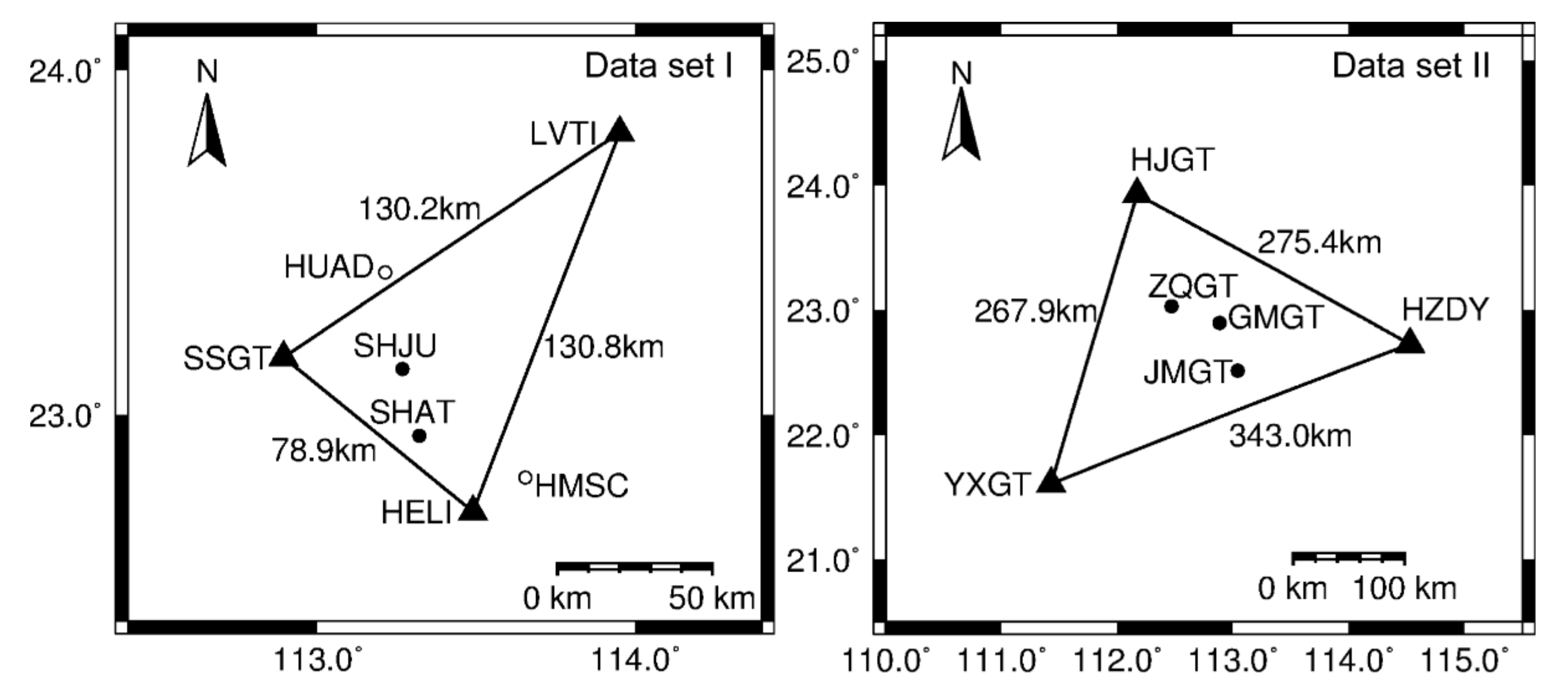
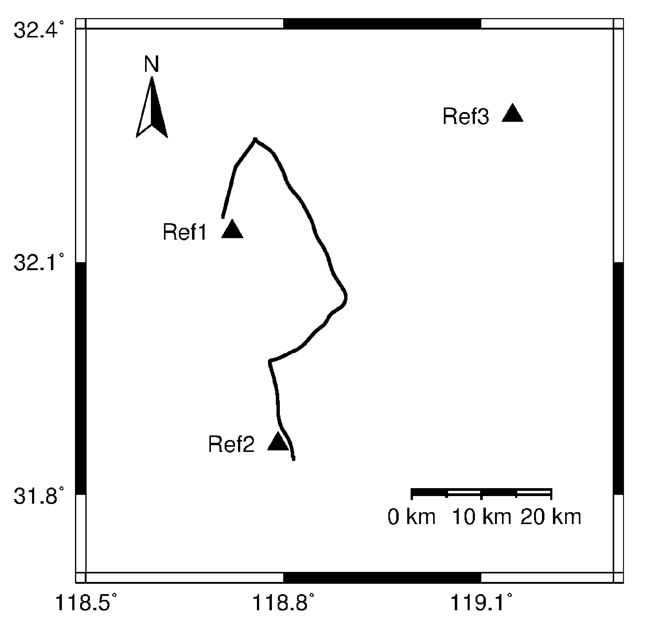
Two sets of data, defined as Data set I and Data set II, were selected in the Guangdong Province of China, as shown in Figure 2. The data were collected from 00:00:00 to 23:59:59 (UTC, Universal Time Coordinated) on day of year 77, 2019 (18 March 2019), and from 00:00:00 to 23:59:59 (UTC) on day of year 112, 2019 (22 April 2019), respectively. The sampling interval was set as 1 s, and the cut-off angle was set at 10°. In Data set I, the stations LVTI, HELI and SSGT were chosen as the reference stations to form a triangle network, and the other four stations were selected as the user stations. The stations SHAT and SHJU are located inside the network, while the stations HUAD and HMSC are outside. In Data set II, the stations HJGT, HZDY and YXGT were chosen as the reference stations, and the other three stations ZQGT, GMGT and JMGT were selected as the user stations. The GAMIT/GLOBK 10.6 software developed by Massachusetts Institute of Technology, Cambridge, MA, USA. [39,40], was used to obtain precise coordinates for all stations as the reference true values.
The network real-time differential positioning results were used to evaluate the performance of different position estimation methods. The traditional algorithm in the range domain and the improved algorithm in the position domain were denoted as RD and PD, respectively. The performances of GPS + BDS and GPS-only solutions were compared as well. The position errors between the network real-time differential positioning results and the true values were calculated. The root mean square (RMS) errors, the standard deviation (STD) values and the percentages of the position errors falling within predefined thresholds of ±0.25 m, ±0.5 m and ±1 m were discussed.
The thresholds were derived from Przestrzelski et al. [17], where it is indicated that most of the position errors in the network real-time differential positioning are smaller than 1 m, and the positioning accuracy are around 0.25 m in the north (N) and east (E) components, and 0.5 m in the up (U) component. Moreover, the 0.5 m threshold also coincides with the positioning accuracy requirement of “Where in Lane” in connected and autonomous vehicles [41].

3.1.1. Data Set I

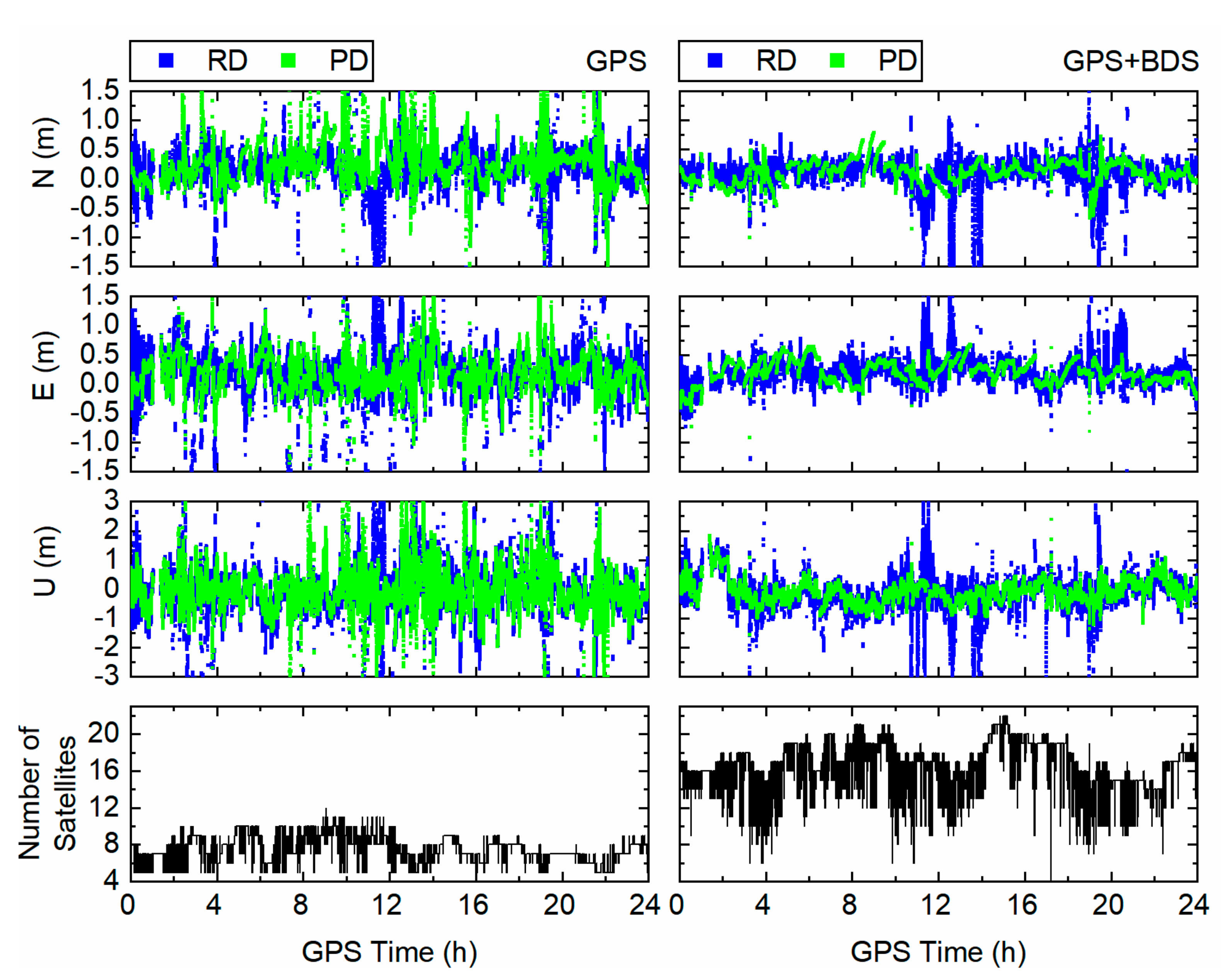
Figure 3 shows the position errors of the network real-time differential positioning and the number of observed satellites for station SHAT. The position errors of position domain (PD) fluctuate smaller than those of range domain (RD), even in the periods when observed satellites changed frequently. The variable number of observed satellites affects the smoothing window of RD and leads to many re-initializations, while PD performs successively with a sufficient number of observed satellites.
For both PD and RD, most of the position errors of GPS-only solution fluctuate from –1 m to 1 m in the N and E components, and from −2 m to 2 m in the U component. Obviously smaller position errors can be found in GPS + BDS solution, since the number of satellites in GPS + BDS solution are significantly larger than those in GPS-only solution.
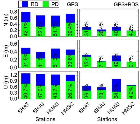
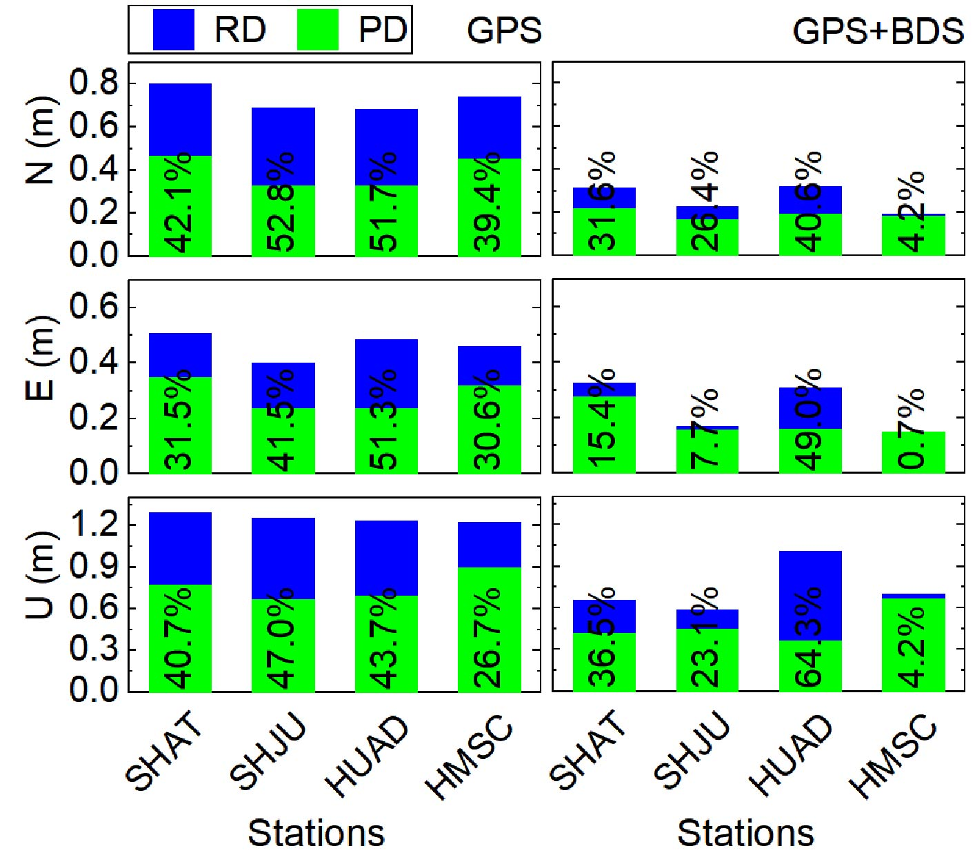
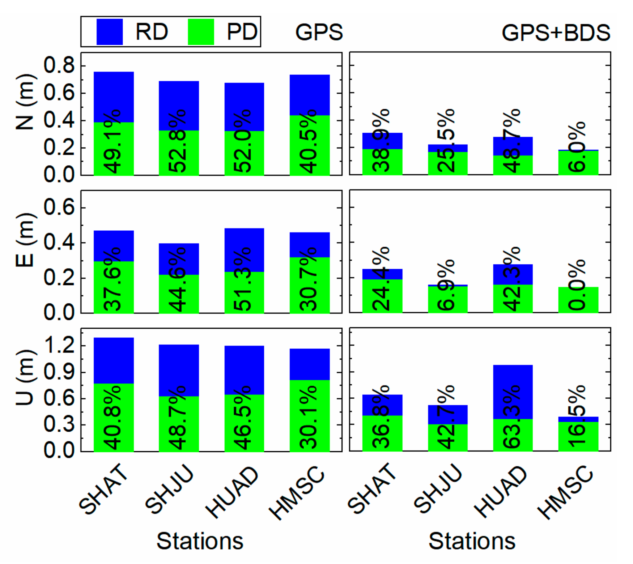
The RMS errors of the network real-time differential positioning for each user station are illustrated in Figure 4. Recall that the first two stations are inside the network. Generally speaking, the RMS errors of PD are smaller than those of RD, in other words, better positioning accuracy can be achieved using PD. Further, for both PD and RD, the RMS errors of GPS + BDS solution are smaller than those of GPS-only solution. The RMS errors of GPS + BDS solution are usually smaller than 0.3 m, 0.3 m and 0.9 m in the N, E and U components, respectively.
Specifically, in GPS-only solution, the maximum improvement of RMS errors can be found in the N component for station SHJU, with a value of 52.8%, when replacing RD with PD. The corresponding value in GPS + BDS solution is 64.3% in the U component for station HUAD.
In addition, the RMS errors of the stations outside and inside the network have little difference, whether in GPS-only or GPS + BDS solution. This may be attributed to the short distances between the outside user stations and their neighboring reference stations.
Table 1 shows the RMS errors according to the types of user stations. Remarkable improvements can be found for PD compared with RD. The overall improvements are about 37.4%, 30.9% and 37.3% in the N, E and U components, respectively. For both PD and RD, the RMS errors of GPS + BDS solution are significantly smaller than those of GPS-only solution. The RMS errors of GPS + BDS solution are 0.269 m, 0.251 m and 0.753 m for RD in the N, E and U components, and 0.190 m, 0.191 m and 0.487 m for PD.
The improvements of GPS + BDS solution with respect to GPS-only solution using PD are about 24%–50%, and the corresponding improvements using RD are about 30%–60%. This, in turn, implies that less accuracy decrease can be found using PD when replacing GPS + BDS solution with GPS-only solution. In particular, the improvements of RMS errors when replacing RD with PD are 13.7%–38.1% in GPS + BDS solution, while the corresponding improvements in GPS-only solution increase. It is also indicated that PD is less affected by the satellite constellation.
The RMS errors for the inside and outside user stations have little difference. Since the outside user stations HUAD and HMSC are very close to the reference stations SSGT and HELI, respectively, their correction accuracy is comparable to that of the inside user stations.
The STD values of the network real-time differential positioning for each user station are shown in Figure 5. An obvious decrease of STD values occurred when replacing RD with PD. The maximum improvement of PD with respect to RD can reach up to 63.3%. Similar to Figure 4, for both PD and RD, remarkable improvements can also be found when using GPS + BDS solution instead of GPS-only solution. The STD values of GPS + BDS solution are smaller than 0.3 m, 0.3 m and 0.9 m in the N, E and U components, respectively.
Table 2 gives the STD values for the inside, the outside and all user stations. The STD values of PD are much smaller than those of RD. For all user stations, the improvements are about 37.7%, 30.9% and 40.9% in the N, E and U components, respectively. For both PD and RD, a significant decrease can be found when replacing GPS-only solution with GPS + BDS solution. The STD values of GPS + BDS solution are 0.265 m, 0.242 m and 0.745 m for RD in the N, E and U components, and 0.188 m, 0.187 m and 0.437 m for PD.
Improvements of GPS + BDS solution with respect to GPS-only solution are about 20%–50% for PD, and about 30%–66% for RD. Specifically, the improvements of PD over RD are 39.1%–48.6% in GPS-only solution, which are larger than those in GPS + BDS solution. This is consistent with the results in Table 1, and further shows that PD is less affected by the satellite constellation.
In addition, the STD values for the outside user stations are similar with those for the inside ones, which also attributes to the close position relation between the outside user station and network.
The percentages of the position errors falling within predefined thresholds are given in Table 3 according to the types of user stations. From the table, one can see that the percentages of the position errors of PD are larger than those of RD in almost all thresholds.
For both PD and RD, the percentage of position errors in each threshold has a higher value when using GPS + BDS solution instead of GPS-only solution. In GPS + BDS solution, the percentages of the position errors falling within ±1 m in the N, E and U components are 96.4%, 99.4% and 89.4% for RD, and 99.4%, 100.0% and 96.7% for PD.
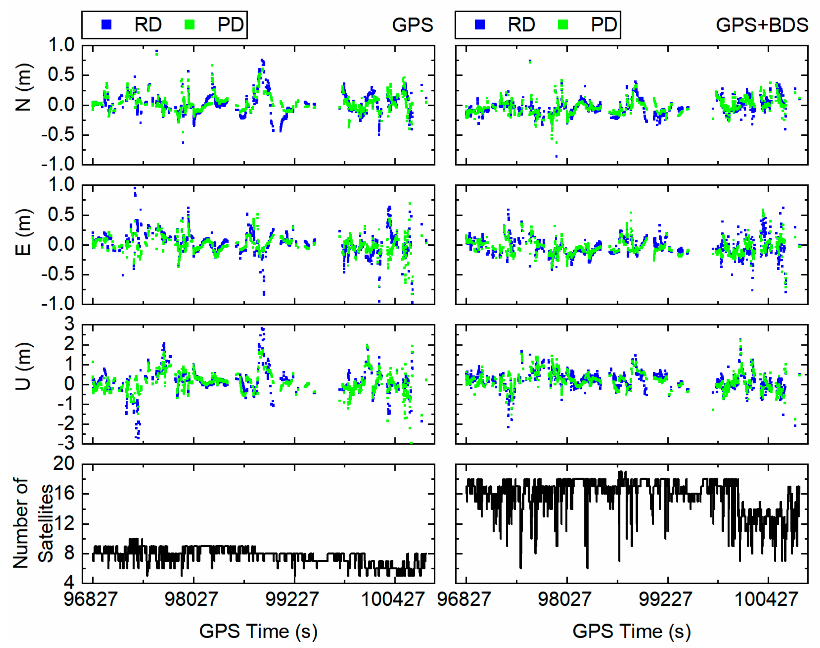
3.1.2. Data Set II

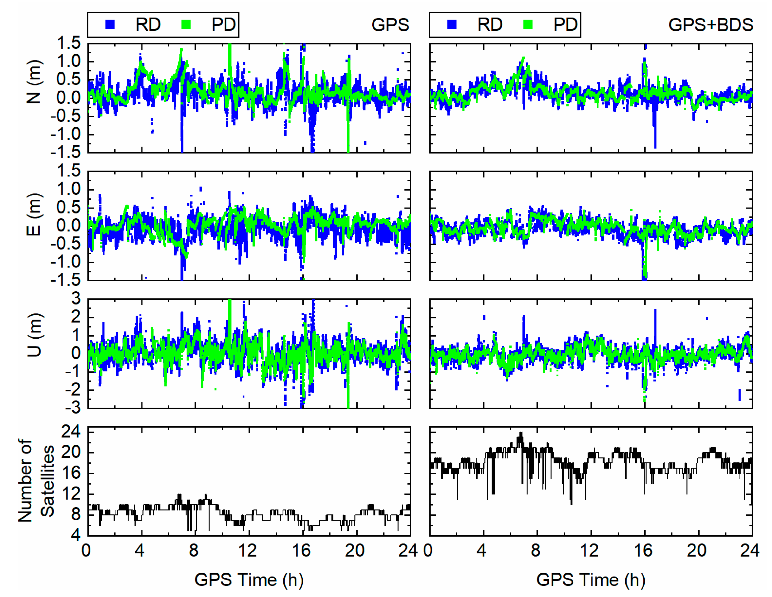
Figure 6 shows the position errors of the network real-time differential positioning and the number of observed satellites for station ZQGT. The position errors of PD fluctuate less than those of RD. For both PD and RD, the position errors of GPS + BDS solution are smaller than those of GPS-only solution. This is consistent with the results in Figure 3.
The position errors of GPS-only solution in this figure are significantly smaller than those in Figure 3, for both PD and RD. This is attributed to the more stable and larger number of observed GPS satellites in Data set II. In GPS + BDS solution, the difference of position error fluctuation between Figure 6 and Figure 3 is small for PD, but large for RD. Since the sufficient number of satellites guarantees the performance of PD for both two figures, the varying number of satellites in Figure 3 restricts the performance of RD.
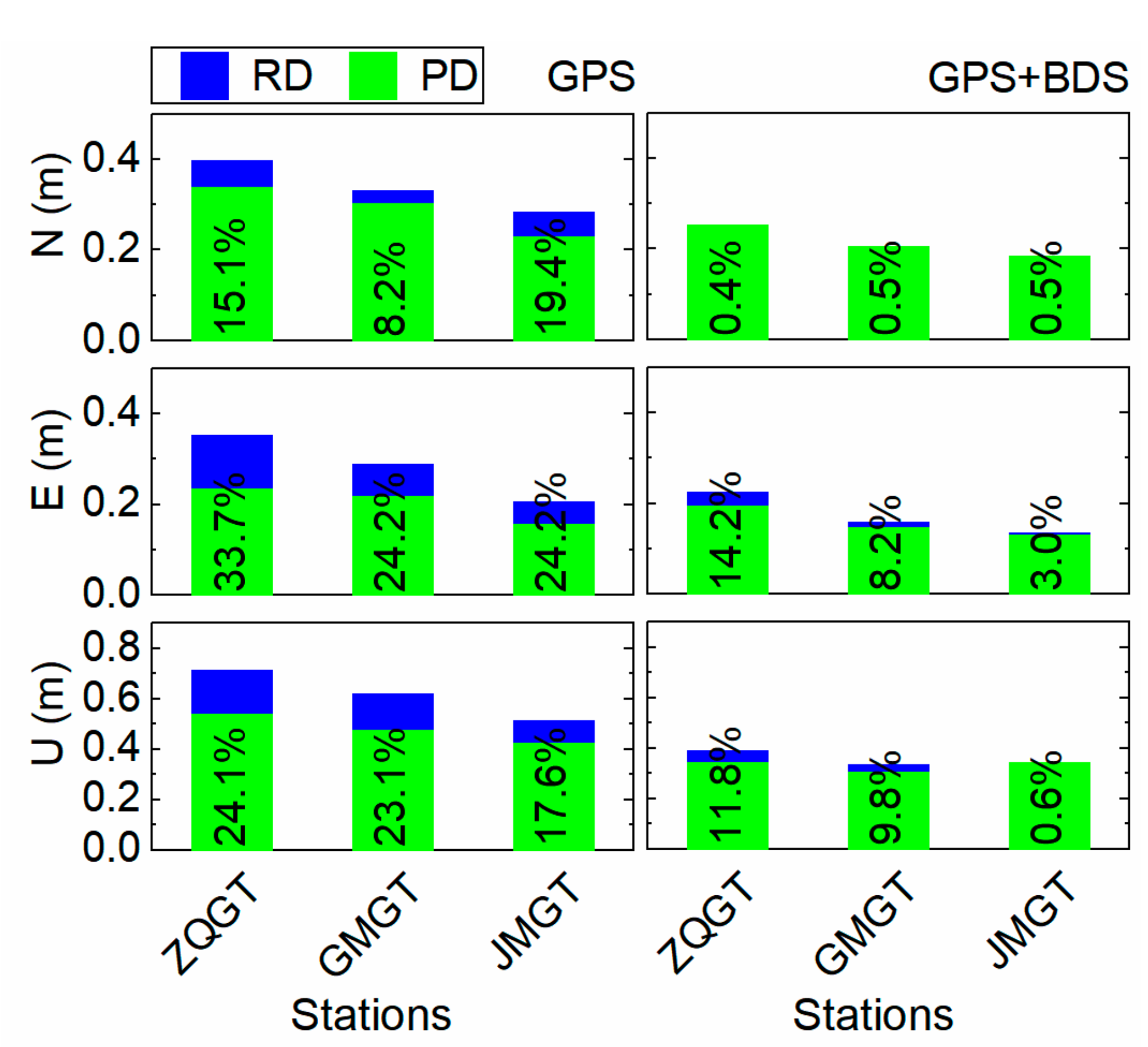
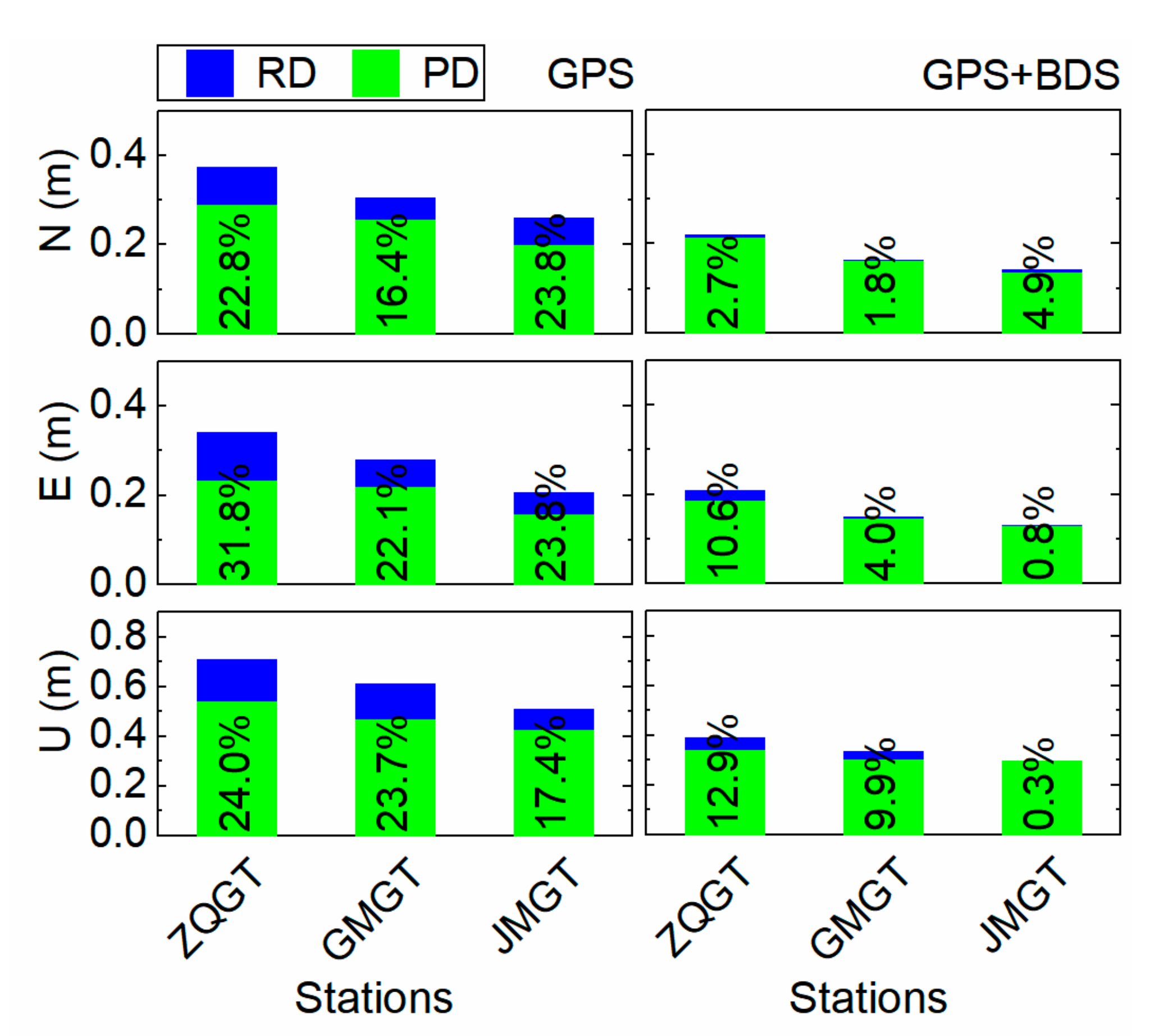
The RMS errors of the network real-time differential positioning for each user station in Data set II are illustrated in Figure 7. Similar to Figure 4, the RMS errors of PD are smaller than those of RD, and the RMS errors of GPS + BDS solution are smaller than those of GPS-only solution. The RMS errors of GPS + BDS solution are usually smaller than 0.3 m, 0.25 m and 0.4 m in the N, E and U components, respectively.
In GPS-only solution, the maximum improvement of RMS errors can be found in the E component for station ZQGT, with a value of 33.7%, when replacing RD with PD. The corresponding value in GPS + BDS solution is 14.2% in the E component for station ZQGT. The improvements of PD over RD in GPS-only solution are larger than those in GPS + BDS solution. Further, the improvements of PD over RD in Figure 7 are smaller than those in Figure 4, whether in GPS-only or GPS + BDS solution. This is because the varying observed satellites have a greater impact on RD.
The STD values of the network real-time differential positioning for each user station in Data set II are shown in Figure 8. The STD values of PD are smaller than those of RD, and the STD values of GPS + BDS solution are smaller than those of GPS-only solution. Remarkable improvements of PD over RD can be found when using GPS-only solution. Moreover, the improvements of PD with respect to RD in Figure 8 are smaller than those in Figure 5.
Table 4 gives the RMS errors and STD values for all user stations in Data set II. The positioning accuracy and precision of PD are better than those of RD. The overall improvements when replacing RD with PD are about 9.5%, 18.3% and 14.8% in the N, E and U components, respectively, which are smaller than those in Table 1 and Table 2. Further, for both PD and RD, the values in GPS + BDS solution are smaller than those in GPS-only solution. The RMS errors of GPS + BDS solution for PD are 0.217 m, 0.159 m and 0.330 m in the N, E and U components, respectively, and the corresponding STD values are 0.173 m, 0.155 m and 0.319 m.
The improvements of GPS + BDS solution over GPS-only solution are about 20%–30% for PD, and about 35%–43% for RD. Moreover, the improvements of PD over RD in GPS + BDS solution are smaller than those in GPS-only solution. It is also indicated that PD is less affected by the satellite constellation.
The percentages of the position errors falling within predefined thresholds are given in Table 5 for all user stations in Data set II. It can be seen that the percentages of the position errors of PD are larger than those of RD in almost all thresholds. For both PD and RD, the percentage of the position errors of GPS + BDS solution is larger than that of GPS-only solution in each threshold.

3.2. Dynamic Experiment

A dynamic experiment was conducted in the Jiangsu Province of China. The data were collected from 2:53:47 to 3:59:59 (UTC) on day of year 112, 2019 (22 April 2019). The sampling interval was set as 1 s, and the cut-off angle was set at 10°. The locations of three reference stations Ref1, Ref2 and Ref3 are shown in Figure 9, as well as the trajectory of the dynamic user station. The GAMIT/GLOBK 10.6 software [39,40] was used to obtain precise coordinates for the three reference stations. The centimeter-level accuracy reference coordinates of the dynamic user station were computed by the GPS real-time kinematic positioning (RTK) using forward and backward filters. It should be pointed out that only the GPS RTK solutions with fixed integer ambiguities were adopted as the reference true values. The network real-time differential positioning results were used to evaluate the performance of PD and RD. The performances of GPS + BDS and GPS-only solutions were compared as well. The same statistical analysis methods used in the static experiment were applied.
Figure 10 shows the position errors of the network real-time differential positioning and the number of observed satellites for the dynamic user station. The position errors of PD fluctuate less than those of RD. Further, for both PD and RD, the position errors of GPS + BDS solution are smaller than those of GPS-only solution. Most of the position errors of GPS + BDS solution are within 0.5 m in the N and E components, and 1.5 m in the U component. The breaks in this figure are due to the discontinuous reference coordinates. In this experiment, only the GPS RTK solutions with fixed integer ambiguities participate in the results analysis, and the epochs with unfixed GPS RTK solutions are excluded, which leads to the interruption of the position errors.
The statistic results of the network real-time differential positioning for the dynamic user are given in Table 6. Significant improvements can be seen when using PD instead of RD. The overall improvements are about 14.4%, 18.5% and 13.8% in the N, E and U components, respectively. For both PD and RD, the RMS errors and STD values of GPS + BDS solution are smaller than those of GPS-only solution. The RMS errors of GPS + BDS solution for PD are 0.122 m, 0.133 m and 0.432 m in the N, E and U components, respectively, and the corresponding STD values are 0.117 m, 0.119 m and 0.397 m.
The improvements of RMS errors and STD values when replacing GPS-only solution with GPS + BDS solution are about 2.5%–10% and 13%–16% for PD, and about 14%–26% and 19%–32% for RD. The improvements of PD over RD in GPS-only solution are larger than those in GPS + BDS solution, which are consistent with the results of the static experiment. It is also demonstrated that PD is less affected by the satellite constellation.
Table 7 shows the percentages of the position errors falling within predefined thresholds for the dynamic user station. About 100%, 100% and 95% of the position errors falling within ±1 m in the N, E and U components, respectively; and at least 97% of the position errors falling within ±0.5 m in the N and E components, respectively.
It can be seen that the percentages of the position errors of PD are larger than those of RD in most of the thresholds, especially in the small thresholds. For both PD and RD, the values of GPS + BDS solution are almost larger than those of GPS-only solution.

4. Discussion

GPS + BDS network real-time differential positioning using a position domain estimation method was studied in this paper. Beneficial results were obtained to show the superiority of GPS + BDS solution and PD. This contribution will enrich the application of network real-time differential positioning in the meter and sub-meter level’s navigation. Furthermore, in the scenarios where gross errors often happen or ambiguity cannot be correctly fixed, the network real-time differential positioning can also provide a potential solution [42].
The results of the experiments show that the performance of network real-time differential positioning using PD is better than that using RD. PD performs consistently even when observed satellites change frequently, as it is immune to the smoothing window and only depends on the number of available satellites. Further, it is demonstrated that PD is less affected by the satellite constellation, since the improvements of PD over RD are more obvious in GPS-only solution, and the improvements of GPS + BDS solution with respect to GPS-only solution are greater in RD, as shown in Table 1, Table 2, Table 4 and Table 6. To verify this feature more intuitively, Table 8 gives the increases of the RMS errors and STD values of PD and RD when using GPS-only solution instead of GPS + BDS solution. The degrees of accuracy and precision decreases of PD are significantly smaller than those of RD, which confirms the previous inference.
The possible reasons why PD is less affected by the satellite constellation than RD would be: (1) the calculated position variation is accurate enough using GPS-only solution and will not be improved much more if replaced by GPS + BDS solution. Thus, the difference between GPS + BDS and GPS-only solutions when using PD is mainly attributed to the different number of available satellites; (2) the positioning performance of RD is mainly due to the number of carrier-phase-smoothed pseudorange observations. GPS + BDS solution can provide more carrier-phase-smoothed pseudorange observations, as well as more available satellites, and thus can achieve more significant improvement.
By comparing the outside and inside user stations, one can see that the positioning accuracy variation does not only depend on whether the user is inside or outside the network, but also on the position relation between the user and network.
It should be noted that, using the same weighting strategy for both GPS and BDS satellites is not appropriate in some cases. A proper weighting strategy must be found to provide a better positioning performance of GPS + BDS solution. The least-squares variance component estimation [43], the cross correlations between different frequencies and the time correlations between epochs have been considered to build stochastic models of GPS and BDS [44]. Wu et al. [45] further pointed out that different elevation-dependent models should be used for GEO (Geostationary Earth Orbit), IGSO (Inclined Geosynchronous Satellite Orbit) and MEO (Medium Earth Orbit) satellites in BDS. Following the above researches, a proper stochastic model for GPS + BDS combination will be investigated in the future.
The corrections of the BDS satellite-induced code bias obtained by the model in Zou et al. [28] may be different from those obtained by other models (e.g., the model in Lou et al. [46]). The difference is caused by the different data and methods used in modeling, and it is usually small [47]. Since the BDS IGSO and BDS MEO satellite-induced code biases can almost be canceled by single-differencing between receivers [48], and the maximum theoretical residual of BDS GEO satellite-induced code bias after single-differencing between receivers is only a few centimeters for 300 km baseline [47]; the model differences can hardly influence the differential positioning.

5. Conclusions

An improved position estimation method in the position domain was proposed, and the GPS + BDS network real-time differential positioning using this improved method was evaluated. The results show that:
  • The RMS errors and STD values of the position errors can be reduced by around 10%–40% using the improved method compared with the traditional algorithm in the range domain. The improved method is less affected by the satellite constellation.
  • The positioning accuracy and availability of GPS + BDS solution is better than those of GPS-only solution, owing to the increasing number of observed satellites. The RMS errors of GPS + BDS network real-time differential positioning using the improved method can reach up to 0.217 m, 0.159 m and 0.330 m in the N, E and U components, respectively, for the static user station, and 0.122 m, 0.133 m and 0.432 m for the dynamic user station.
  • The positioning accuracy variation does not only depend on whether the user is inside or outside the network, but also on the position relation between the user and network.
It should be noted that the assumed precision of GPS and BDS code and carrier phase measurements may not be that realistic, and the stochastic model using the same elevation-dependent model for each satellite type may not be that appropriate. An investigation to obtain the proper weighting strategy for GPS and BDS satellites will be made.

Author Contributions

Conceptualization, J.C. and W.T.; formal analysis, J.C., R.Y., C.D., Q.L. and Y.L.; investigation, R.Y., X.Z., M.S. and Y.W.; methodology, J.C. and W.T.; software, J.C.; writing—original draft, J.C.; writing—review and editing, C.D. and W.T..

Funding

This research was funded by the National Key Research and Development Program of China (Grant No. 2017YFB0503702), National Natural Science Foundation of China (Grant Nos. 41874037, 41804028), “the Fundamental Research Funds for the Central Universities” (Grant No. 2042018gf0001) and the Wuhan Science and Technology Project (Grant No. 2018010401011271).

Acknowledgments

We are very grateful to Mengtang Hui at the North Information Control Institute Group Co., Ltd. for the dynamic data. We thank the anonymous reviewers for their constructive comments and suggestions.

Conflicts of Interest

The authors declare no conflicts of interest.

Appendix A

The stations HUAD and SHAT in the Guangdong Province of China were selected. The data were collected from 00:00:00 to 23:59:59 (UTC) on day of year 77, 2019 (18 March 2019). The sampling interval was set as 1 s, and the cut-off angle was set at 10°. Figure A1 shows the difference of the unit vectors in adjacent epochs for each station. It can be seen that most of the values are smaller than 1.0 × 10⁻⁴, 1.0 × 10⁻⁴ and 1.5 × 10⁻⁴ in the X, Y and Z components, respectively. Since the positioning accuracy of the network real-time differential positioning is a few decimeters, the first term on the right side of Equation (9) is usually smaller than 0.35 mm, which cannot influence the position variation estimation. Further, the values of GEO are almost equal to zero, the values of IGSO vary from −0.5 × 10⁻⁴ to 0.5 × 10⁻⁴, and the values of MEO are a little larger. This may be attributed to the different velocity of the satellite relative to the ground.
Figure A1. Difference of the unit vectors in adjacent epochs for each station. Left panels: HUAD; right panels: SHAT.
Remotesensing 11 01480 g0a1

References

  1. Development of the BeiDou Navigation Satellite System (Version 3.0). Available online: http://www.beidou.gov.cn/xt/gfxz/201812/P020190117356387956569.pdf (accessed on 25 February 2019).
  2. Deng, C.; Tang, W.; Liu, J.; Shi, C. Reliable single-epoch ambiguity resolution for short baselines using combined GPS/BeiDou system. GPS Solut. 2014, 18, 375–386. [Google Scholar] [CrossRef]
  3. Gao, W.; Gao, C.; Pan, S.; Meng, X.; Xia, Y. Inter-System Differencing between GPS and BDS for Medium-Baseline RTK Positioning. Remote Sens. 2017, 9, 948. [Google Scholar] [CrossRef]
  4. Tu, R.; Zhang, P.; Zhang, R.; Lu, C.; Liu, J.; Lu, X. The study and realization of BDS un-differenced network-RTK based on raw observations. Adv. Space Res. 2017, 59, 2809–2818. [Google Scholar] [CrossRef]
  5. Xu, Y.; Wu, C.; Li, L.; Yan, L.; Liu, M.; Wang, S. GPS/BDS Medium/Long-Range RTK Constrained with Tropospheric Delay Parameters from NWP Model. Remote Sens. 2018, 10, 1113. [Google Scholar] [CrossRef]
  6. Li, X.; Guo, J.; Zhou, L. Performance analysis of BDS/GPS kinematic vehicle positioning in various observation conditions. Sensor Rev. 2016, 36, 249–256. [Google Scholar] [CrossRef]
  7. Zhou, K.; Wang, L.; Yuan, C.; Yuan, H.; Zhao, J.; Li, Z. Influence of the time-delay of correction for BDS and GPS combined real-time differential positioning. Electron. Lett. 2016, 52, 1063–1065. [Google Scholar] [CrossRef]
  8. Tang, W.; Cui, J.; Hui, M.; Deng, C. Performance analysis for BDS phase-smoothed pseudorange differential positioning. J. Navig. 2016, 69, 1011–1023. [Google Scholar] [CrossRef]
  9. Odijk, D.; Wanninger, L. Differential Positioning. In Springer Handbook of Global Navigation Satellite Systems; Teunissen, P., Montenbruck, O., Eds.; Springer International Publishing: Berlin, Germany, 2017; Chapter 26; pp. 753–780. [Google Scholar]
  10. Specht, C. Accuracy and coverage of the modernized Polish Maritime differential GPS system. Adv. Space Res. 2011, 47, 221–228. [Google Scholar] [CrossRef]
  11. Vu, A.; Ramanandan, A.; Chen, A.; Farrell, J.A.; Barth, M. Real-Time Computer Vision/DGPS-Aided Inertial Navigation System for Lane-Level Vehicle Navigation. IEEE Trans. Intell. Transp. 2012, 13, 899–913. [Google Scholar] [CrossRef]
  12. Patel, A.; Katiyar, S.K.; Prasad, V. Performances evaluation of different open source DEM using Differential Global Positioning System (DGPS). Egypt. J. Remote Sens. Space Sci. 2016, 19, 7–16. [Google Scholar] [CrossRef] [Green Version]
  13. Oh, K.R.; Kim, J.C.; Nam, G.W. Development of navigation algorithm to improve position accuracy by using multi-DGPS reference stations’ PRC information. J. Glob. Position Syst. 2005, 4, 144–150. [Google Scholar] [CrossRef]
  14. Bakuła, M. Network code DGPS positioning and reliable estimation of position accuracy. Surv. Rev. 2010, 42, 82–91. [Google Scholar] [CrossRef]
  15. Nejat, D.; Kiamehr, R. An investigation on accuracy of DGPS network-based positioning in mountainous regions, a case study in Alborz network. Acta Geod. Geophys. 2013, 48, 39–51. [Google Scholar] [CrossRef]
  16. Weng, D.; Ji, S.; Chen, W.; Li, Z.; Xu, Y.; Ye, L. Assessing and mitigating the effects of the ionospheric variability on DGPS. GPS Solut. 2015, 19, 107–116. [Google Scholar] [CrossRef]
  17. Przestrzelski, P.; Bakuła, M.; Galas, R. The integrated use of GPS/GLONASS observations in network code differential positioning. GPS Solut. 2017, 21, 627–638. [Google Scholar] [CrossRef]
  18. Hatch, R. The synergism of GPS code and carrier measurements. In Proceedings of the Third International Geodetic Symposium on Satellite Doppler Positioning, New Mexico State University, Las Cruces, NM, USA, 8–12 February 1982; pp. 1213–1231. [Google Scholar]
  19. Hwang, P.Y.; Mcgraw, G.A.; Bader, J.R. Enhanced differential GPS carrier-smoothed code processing using dual-frequency measurements. Navigation 1999, 46, 127–137. [Google Scholar] [CrossRef]
  20. Park, B.; Sohn, K.; Kee, C. Optimal Hatch filter with an adaptive smoothing window width. J. Navig. 2008, 61, 435–454. [Google Scholar] [CrossRef]
  21. Liu, X.; Yang, S.; Yang, J.; Lu, P. Optimal Doppler-Aided Autonomous Position with a Flexible Smoothing Window Width. In Proceedings of the 26th International Technical Meeting of the Satellite Division of The Institute of Navigation (ION GNSS+ 2013), Nashville Convention Center, Nashville, TN, USA, 16–20 September 2013; pp. 3521–3527. [Google Scholar]
  22. Zhou, Z.; Li, B. Optimal Doppler-aided smoothing strategy for GNSS navigation. GPS Solut. 2017, 21, 197–210. [Google Scholar] [CrossRef]
  23. Hwang, P.Y.; Brown, R.G. GPS navigation: Combining pseudorange with continuous carrier phase using a Kalman filter. Navigation 1990, 37, 181–296. [Google Scholar] [CrossRef]
  24. Bisnath, S.B.; Langley, R.B. Precise, efficient GPS-based geometric tracking of low earth orbiters. In Proceedings of the 55th Annual Meeting of The Institute of Navigation (1999), Royal Sonesta Hotel, Cambridge, MA, USA, 27–30 June 1999; pp. 751–760. [Google Scholar]
  25. Bisnath, S.B.; Langley, R.B. High-precision platform positioning with a single GPS receiver. In Proceedings of the 14th International Technical Meeting of the Satellite Division of the Institute of Navigation (ION GPS 2001), Salt Palace Convention Center, Salt Lake City UT, USA, 11–14 September 2001; pp. 2585–2593. [Google Scholar]
  26. Lee, H.K.; Rizos, C.; Jee, G.I. Design of kinematic DGNSS filters with consistent error covariance information. IEEE Proc. Radar Sonar Navig. 2004, 151, 382–388. [Google Scholar] [CrossRef] [Green Version]
  27. Soon, B.K.H.; Scheding, S.; Lee, H.; Lee, H.; Durrant-Whyte, H. An approach to aid INS using time-differenced GPS carrier phase (TDCP) measurements. GPS Solut. 2008, 12, 261–271. [Google Scholar] [CrossRef]
  28. Zou, X.; Li, Z.; Li, M.; Tang, W.; Deng, C.; Chen, L.; Wang, C.; Shi, C. Modeling BDS pseudorange variations and models assessment. GPS Solut. 2017, 21, 1661–1668. [Google Scholar] [CrossRef]
  29. Zhang, X.; Li, X.; Lu, C.; Wu, M.; Pan, L. A comprehensive analysis of satellite-induced code bias for BDS-3 satellites and signals. Adv. Space Res. 2019, 63, 2822–2835. [Google Scholar] [CrossRef]
  30. National Geodetic Survey. Available online: https//www.ngs.noaa.gov/ANTCAL/ (accessed on 27 April 2019).
  31. Townsend, B.; Fenton, P. A Practical Approach to the Reduction of Pseudorange Multipath Errors in a Ll GPS Receiver. In Proceedings of the 7th International Technical Meeting of the Satellite Division of The Institute of Navigation (ION GPS 1994), Salt Palace Convention Center, Salt Lake City UT, USA, 20–23 September 1994; pp. 143–148. [Google Scholar]
  32. Cai, C.; Gao, Y.; Pan, L.; Dai, W. An analysis on combined GPS/COMPASS data quality and its effect on single point positioning accuracy under different observing conditions. Adv. Space Res. 2014, 54, 818–829. [Google Scholar] [CrossRef]
  33. RTCA Inc. Minimum Aviation System Performance Standards for the Local Area Augmentation System (LAAS); RTCA/DO-245; RTCA Inc.: Washington, DC, USA, 1998. [Google Scholar]
  34. Wanninger, L. Improved ambiguity resolution by regional differential modelling of the ionosphere. In Proceedings of the 8th International Technical Meeting of the Satellite Division of The Institute of Navigation (ION GPS 1995), Palm Springs, CA, USA, 12–15 September 1995; pp. 55–62. [Google Scholar]
  35. Swider, R.; Kaser, K.; Braff, R. Recent Developments in the LAAS Program. In Proceedings of the Position Location and Navigation Symposium IEEE 1998, Palm Springs, CA, USA, 20–23 April 1998; pp. 441–470. [Google Scholar]
  36. Yang, Y.; Li, J.; Wang, A.; Xu, J.; He, H.; Guo, H.; Shen, J.; Dai, X. Preliminary assessment of the navigation and positioning performance of BeiDou regional navigation satellite system. Sci. China Earth Sci. 2014, 57, 144–152. [Google Scholar] [CrossRef]
  37. Teunissen, P.J.G. The GPS phase-adjusted pseudorange. In Proceedings of the 2nd International Workshop on High Precision Navigation, Stuttgart, Freudenstadt, Germany, 12–15 November 1991; pp. 115–125. [Google Scholar]
  38. Gelb, A.; Kasper, J.F.; Nash, R.A.; Price, C.F.; Sutherland, A.A. Applied Optimal Estimation; MIT Press: Cambridge, MA, USA, 2001. [Google Scholar]
  39. Herring, T.A.; Floyd, M.A.; King, R.W.; McClusky, S.C. GLOBK Reference Manual, Global Kalman Filter VLBI and GPS Analysis Program, Release 10.6; Massachusetts Institute of Technology: Cambridge, MA, USA, 2015. [Google Scholar]
  40. Herring, T.A.; King, R.W.; Floyd, M.A.; McClusky, S.C. GAMIT Reference Manual, GPS Analysis at MIT, Release 10.6; Massachusetts Institute of Technology: Cambridge, MA, USA, 2015. [Google Scholar]
  41. Meng, X.; Roberts, S.; Cui, Y.; Gao, Y.; Chen, Q.; Xu, C.; He, Q.; Sharples, S.; Bhatia, P. Required navigation performance for connected and autonomous vehicles: Where are we now and where are we going? Transport. Plan. Technol. 2018, 41, 104–118. [Google Scholar] [CrossRef]
  42. Bakuła, M. Static network code DGPS positioning vs. carrier phase single baseline solutions for short observation time and medium-long distances. Artif. Satell. 2007, 42, 167–183. [Google Scholar] [CrossRef]
  43. Teunissen, P.J.G.; Amiri-Simkooei, A.R. Least-squares variance component estimation. J. Geod. 2008, 82, 65–82. [Google Scholar] [CrossRef]
  44. Li, B. Stochastic modeling of triple-frequency BeiDou signals: Estimation, assessment and impact analysis. J. Geod. 2016, 90, 593–610. [Google Scholar] [CrossRef]
  45. Wu, S.; Zhao, X.; Pang, C.; Zhang, L.; Wang, Y. A new strategy of stochastic modeling aiming at BDS hybrid constellation in precise relative positioning. Adv. Space Res. 2019, 63, 2757–2770. [Google Scholar] [CrossRef]
  46. Lou, Y.; Gong, X.; Gu, S.; Zheng, F.; Feng, Y. Assessment of code bias variations of BDS triple-frequency signals and their impacts on ambiguity resolution for long baselines. GPS Solut. 2017, 21, 177–186. [Google Scholar] [CrossRef]
  47. Tang, W.; Liu, Q.; Gao, K.; Deng, C.; Cui, J.; Shen, M. Influence of BDS pseudorange code biases on baseline resolution. Geomat. Inf. Sci. Wuhan Univ. 2018, 1199–1206. (In Chinese) [Google Scholar] [CrossRef]
  48. Zhang, X.; He, X.; Liu, W. Characteristics of systematic errors in the BDS Hatch–Melbourne–Wübbena combination and its influence on wide-lane ambiguity resolution. GPS Solut. 2017, 21, 265–277. [Google Scholar] [CrossRef]
Figure 1. Flow chart of the network real-time differential positioning using the improved algorithm.
Remotesensing 11 01480 g001
Figure 2. Geographical distribution of the stations in the static experiment (left: Data set I; right: Data set II). Black solid triangles represent the reference stations. Black solid and hollow circles denote the user stations inside and outside the network, respectively.
Remotesensing 11 01480 g002
Figure 3. Position errors of the network real-time differential positioning and number of satellites for SHAT. Left panels: Global Positioning System (GPS)-only; right panels: GPS + BDS (BeiDou Navigation Satellite System). PD: position domain, RD: range domain.
Remotesensing 11 01480 g003
Figure 4. Root mean square (RMS) errors of the network real-time differential positioning for each user station in the north (N, top), east (E, middle) and up (U, bottom) components, respectively. Left panels: GPS-only; right panels: GPS + BDS. The percentages on each bar are the improvements of PD over RD.
Remotesensing 11 01480 g004
Figure 5. Standard deviation (STD) values of the network real-time differential positioning for each user station in the N (top), E (middle) and U (bottom) components, respectively. Left panels: GPS-only; right panels: GPS + BDS. The percentages on each bar are the improvements of PD over RD.
Remotesensing 11 01480 g005
Figure 6. Position errors of the network real-time differential positioning and number of satellites for ZQGT. Left panels: GPS-only; right panels: GPS + BDS.
Remotesensing 11 01480 g006
Figure 7. RMS errors of the network real-time differential positioning for each user station in the N (top), E (middle) and U (bottom) components, respectively. Left panels: GPS-only; right panels: GPS + BDS. The percentages on each bar are the improvements of PD over RD.
Remotesensing 11 01480 g007
Figure 8. STD values of the network real-time differential positioning for each user station in the N (top), E (middle) and U (bottom) components, respectively. Left panels: GPS-only; right panels: GPS + BDS. The percentages on each bar are the improvements of PD over RD.
Remotesensing 11 01480 g008
Figure 9. Geographical distribution of the stations in the dynamic experiment. Black solid triangles represent the reference stations Ref1, Ref2 and Ref3. Black line denotes the trajectory of the dynamic user station.
Remotesensing 11 01480 g009
Figure 10. Position errors of the network real-time differential positioning and number of satellites for the dynamic user station. Left panels: GPS-only; right panels: GPS + BDS.
Remotesensing 11 01480 g010
Table 1. RMS errors of the network real-time differential positioning for the inside, the outside and all user stations.
GPSGPS + BDS
NEUNEU
InsideRD (m)0.7480.4581.2780.2750.2590.619
PD (m)0.4010.2970.7210.1930.2230.432
Improvement (%)46.335.143.629.613.730.2
OutsideRD (m)0.7140.4731.2280.2640.2430.867
PD (m)0.3950.2810.8010.1870.1530.537
Improvement (%)44.740.634.829.037.038.1
AllRD (m)0.7310.4661.2530.2690.2510.753
PD (m)0.3980.2890.7620.1900.1910.487
Improvement (%)45.537.939.229.323.835.3
Table 2. STD values of the network real-time differential positioning for the inside, the outside and all user stations.
GPSGPS + BDS
NEUNEU
InsideRD (m)0.7380.4421.2680.2750.2470.615
PD (m)0.3800.2660.7140.1900.2090.414
Improvement (%)48.639.843.731.015.232.7
OutsideRD (m)0.7130.4721.1860.2410.2370.852
PD (m)0.3940.2810.7360.1610.1530.439
Improvement (%)44.840.537.933.035.348.5
AllRD (m)0.7280.4631.2300.2650.2420.745
PD (m)0.3900.2820.7330.1880.1870.437
Improvement (%)46.439.140.429.022.641.3
Table 3. Percentages of the position errors of the network real-time differential positioning in predefined thresholds for the inside, the outside and all user stations. (Unit: %)
NEU
±0.25 m±0.5 m±1 m±0.25 m±0.5 m±1 m±0.5 m±1 m
InsideGPSRD60.087.395.961.887.197.055.983.5
PD61.788.997.965.491.499.462.088.8
Improvement2.81.92.15.84.92.611.06.4
GPS + BDSRD81.491.697.274.595.999.368.393.3
PD82.093.799.674.797.3100.074.398.5
Improvement0.82.32.40.31.40.78.85.6
OutsideGPSRD65.089.996.066.090.296.851.080.6
PD66.190.597.669.495.299.456.286.1
Improvement1.60.71.75.15.62.710.06.8
GPS + BDSRD80.982.695.579.995.299.449.785.4
PD83.586.399.290.199.9100.062.494.8
Improvement3.14.53.912.84.90.625.611.1
AllGPSRD62.688.695.963.988.796.953.482.0
PD63.989.797.867.493.499.459.187.4
Improvement2.21.31.95.55.32.610.56.6
GPS + BDSRD81.287.196.477.295.699.459.089.4
PD82.890.099.482.498.6100.068.496.7
Improvement2.03.33.26.73.20.615.98.2
Table 4. RMS errors and STD values of the network real-time differential positioning for all user stations.
GPSGPS + BDS
NEUNEU
RMSRD (m)0.3400.2890.6190.2190.1770.356
PD (m)0.2930.2050.4810.2170.1590.330
Improvement (%)13.928.922.30.710.17.1
STDRD (m)0.3160.2830.6170.1780.1670.346
PD (m)0.2510.2060.4790.1730.1550.319
Improvement (%)20.627.322.22.96.97.7
Table 5. Percentages of the position errors of the network real-time differential positioning in predefined thresholds for all user stations. (Unit: %)
NEU
±0.25 m±0.5 m±1 m±0.25 m±0.5 m±1 m±0.5 m±1 m
GPSRD72.993.399.181.096.499.275.195.0
PD73.793.499.282.897.799.778.996.1
Improvement1.00.10.12.31.40.65.01.2
GPS + BDSRD79.095.799.887.299.299.886.798.7
PD81.095.799.990.499.599.889.299.3
Improvement2.50.00.13.70.30.02.90.6
Table 6. RMS errors and STD values of the network real-time differential positioning for the dynamic user station.
GPSGPS + BDS
NEUNEU
RMSRD (m)0.1670.1760.6180.1350.1520.456
PD (m)0.1350.1360.4800.1220.1330.432
Improvement (%)18.822.722.49.812.55.4
STDRD (m)0.1660.1750.6100.1300.1420.414
PD (m)0.1340.1360.4690.1170.1190.397
Improvement (%)19.422.423.09.716.44.2
Table 7. Percentages of the position errors of the network real-time differential positioning in predefined thresholds for the dynamic user station. (Unit: %)
NEU
±0.25 m±0.5 m±1 m±0.25 m±0.5 m±1 m±0.5 m±1 m
GPSRD89.298.7100.088.097.899.877.491.7
PD93.799.1100.094.299.199.877.695.6
Improvement5.00.40.07.11.30.00.34.3
GPS + BDSRD95.297.499.991.699.2100.078.695.5
PD96.297.899.996.399.4100.079.895.7
Improvement1.00.40.05.10.20.01.50.2
Table 8. Increases of RMS errors and STD values of GPS-only solution compared with GPS + BDS solution. (Unit: %)
RMSSTD
NEUNEU
StaticRD113.374.270.2126.180.571.7
PD71.940.051.176.441.559.0
DynamicRD23.216.035.528.223.647.1
PD10.82.611.114.414.918.2

