1. Introduction
Synthetic Aperture Radar (SAR) imagery has been widely used in the remote sensing field due to several advantages such as: high resolution, day-and-night acquisition, and cloud-penetrating capabilities [
1]. Despite all these important features, SAR images are inherently affected by a single dependent granular multiplicative noise caused by the interaction out-of-phase waves with a target, called speckle noise. In fact, this phenomenon decreases the utility of satellite images since it reduces the ability to detect ground targets and obscures the recognition of spatial patterns, which leads to a severe decrease of the automated scene’s performances analysis and information extraction techniques [
2].
In order to mitigate the adverse effects caused by speckle noise, several families of approaches have been introduced in the scientific community, for instance: the spatial-based approaches. i.e., Kuan [
3], Lee [
4], and Γ-MAP [
5] filters, the non-local techniques, i.e., PPB-it [
6], SAR-BM3D [
7], NL-SAR [
8], and MuLoG [
9] filtering algorithms, and frequency-based filters including the Wiener Filter (WF) [
10]. Recently, deep learning-based approaches have been gaining interest in the SAR image despeckling field [
11,
12,
13]. Concerning the spatial approaches, proceeding with these techniques does not need too much memory occupation and seems to be important in terms of fast processing time. However, it causes the smoothness of the input SAR image and loss of its most important information. As for non-local approaches, they have been presented as an efficient solution in terms of edges, fine-details, and good resolution preservation, despite the long time computation and the important amount of memory occupied during its processing stage. An effective tentative approach has been done in FANS [
14], where the authors proposed a fast version of the non-local SAR-BM3D approach. However, with very large images, typical of available sensors’ acquisitions, the time can still be a problem. Summarizing, both families suffer from a main limitation: loss of details (the former) and time consumption (the latter).
Considering the previous drawbacks, the idea is to develop a fast speckle filter able to provide an accurate solution within a short time. Therefore, we propose a solution that preserves the main characteristics of SAR images with a fast processing time. In particular, we work on an improvement of the classical WF. In fact, the latter is defined as a frequency-based approach, where the filtering is performed on the whole image based on the power spectra of the noise and of the image. Although WF is identified as a fast processing algorithm, it completely neglects the local (spatial) characteristics of the image. For that, we suggest to modify the kernel of WF properly by introducing, to the previous basic kernel, the information about the spatial characteristics of the image. This information, once estimated, provides us the level of smoothing of the filter for a specific pixel. Moreover, we aim to decrease the processing time elapsed by WF by reducing the complexity of the solution and making it adequate for the Graphics Processing Unit (GPU). Hence, we demonstrate that this procedure not only ameliorates the fast processing time characteristics of the filter, but also that it is able to provide an efficient solution in terms of speckle noise reduction with considerable image detail preservation. Summarizing, the proposed algorithm, thanks to its two main innovative aspects, such as the exploitation of the local characteristics of the image in a frequency domain-based approach and the peculiar implementation specifically designed for a GPU, is able to provide an effective filtering result within a very limited processing time.
The remainder of the paper is structured as follows: In
Section 2, we describe briefly the proposed approach. Next,
Section 3 focuses on introducing the mainly known filters performed for the comparison with our proposed solution, defining the performance indicators used for objectively evaluating the comparison filters and displaying the experimental results related to both the simulated framework and real SAR data in several test cases. As for
Section 4, it discusses and comments on these obtained results. Finally,
Section 5 summarizes the conclusions and outlines future research.
2. Methodology
Let
be the noise-free single-look intensity SAR signal, and let
be the noisy single-look intensity signal. These two signals are related to each other via the following equation:
where
denotes the speckle noise and
are respectively the azimuth and range indexes.
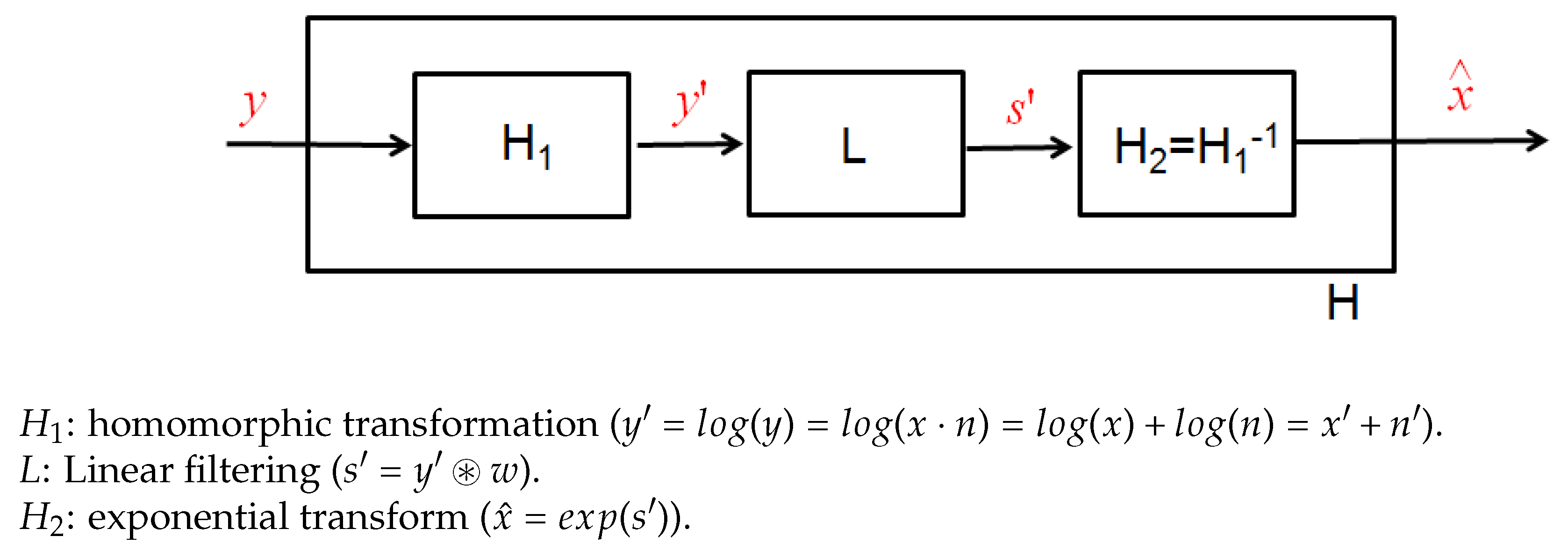
The signal
y faces, at first, a homomorphic transformation, given by the logarithm function, which aims to convert the multiplicative speckle noise to an additive noise
n′. Thus, we obtain a signal
y′ defined as a summation between a noise-free signal
x′ and a noise quantity
n′ in the logarithmic domain. Next,
y′ undergoes into a linear filtering
L, described as a convolution with the Wiener kernel
w, in order to achieve a filtered output
s′. Finally, the latter returns to the initial domain using the exponential transform. The procedure is sketched in
Figure 1.
Let us focus on the linear filtering step (L) in the frequency domain. In the filtering part, the Wiener kernel
W is given by the following formula [
10]:
where
and
denote respectively the power density spectrum of the image and noise. It should be noted that the dependence on the frequency variable has been neglected.
It is possible to retrieve the power spectrum of the noise for the implementation of WF, starting from its Auto-Correlation Function (ACF), as in [
15]. Let us first consider the input noise of Equation (
1). It follows an exponential distribution with mean and variance equal to one. After the transformation of
, the noise changes its distribution, and its mean value becomes:
where
is the Euler constant.
Exploiting the mean value given in Equation (
3), it is possible to write down the auto-correlation function of the noise
n′ as:
where the expectation is calculated using the joint Probability Distribution Function (PDF)
of the noise sample in the pixels
and
.
By making the assumption of decorrelation between noise samples commonly adopted in the literature as for example in [
2,
6,
7], the auto-correlation function becomes the Dirac delta function, whose value in zero is provided by:
The latter is calculated in closed form according to [
16] and [
17], and it represents the ACF of the noise after the transformation of operator
. Since its mean is different from zero, in order to apply the WF, the contribution of the mean has to be eliminated. For this reason, the power spectrum of the noise
n′ is calculated by applying a Fourier Transform (FT) to the ACF after removing the square mean of
n′.
The power spectrum of the unknown image
can be estimated using an iterative procedure as presented in [
18].
Several more sophisticated techniques for the estimation of the power spectrum exist in the literature based on the
-divergence, as [
19], or based on the
-divergence, as [
20]. However, we considered a simple, yet effective approach in order to maintain a limited computational cost and speed up the algorithm.
Although the classical WF is a very fast filtering algorithm, it does not take into account the local characteristics of the image. Thus, the idea is to provide the local information to WF, keeping its good performances in terms of velocity. For that, we propose to modify the Wiener kernel by introducing the contextual information as:
where
is a vector containing K linearly-spaced elements (or weights). The first value of the
vector
is assigned equal to one. It corresponds to the behavior of the classical WF. When
increases, the filter tends to impose a stronger regularization. The idea is to link the values of the
vector with the characteristics of the observed scene. It can be understood that large values of
should correspond to homogeneous areas, and accordingly, the solution of WF in these areas is highly regularized. However, a slight regularization with small values of
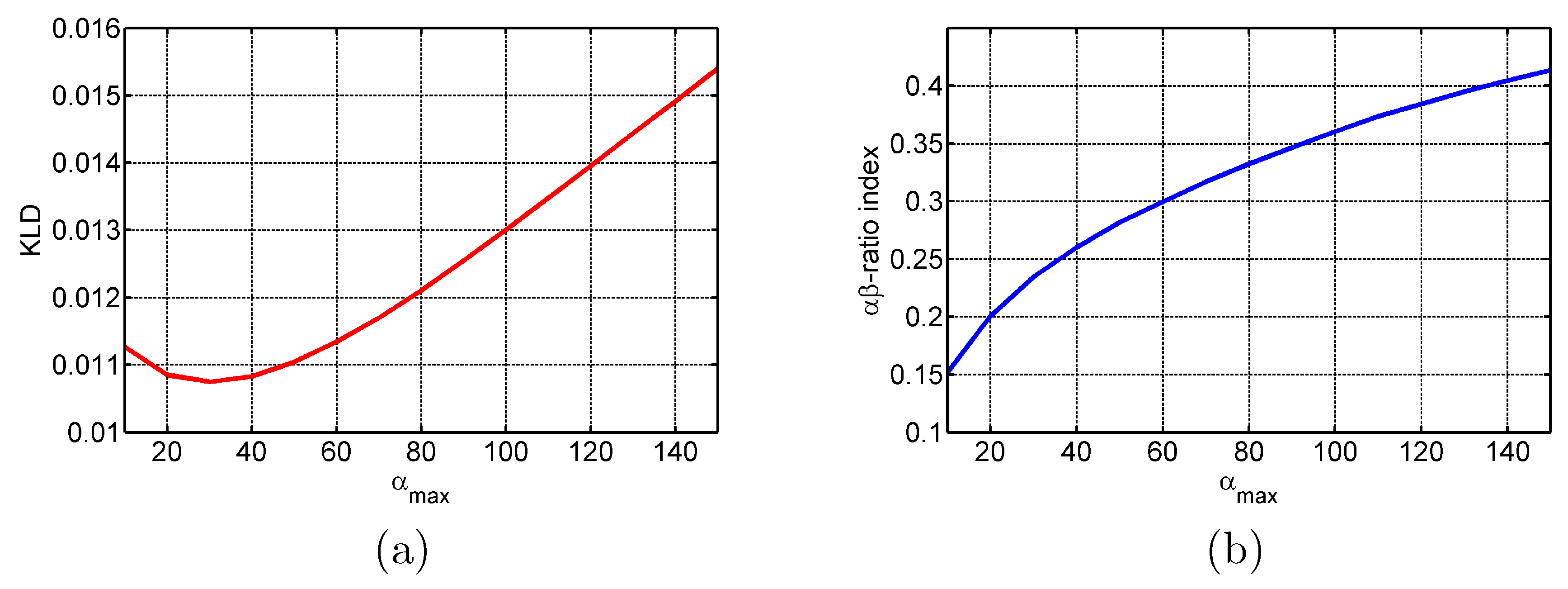
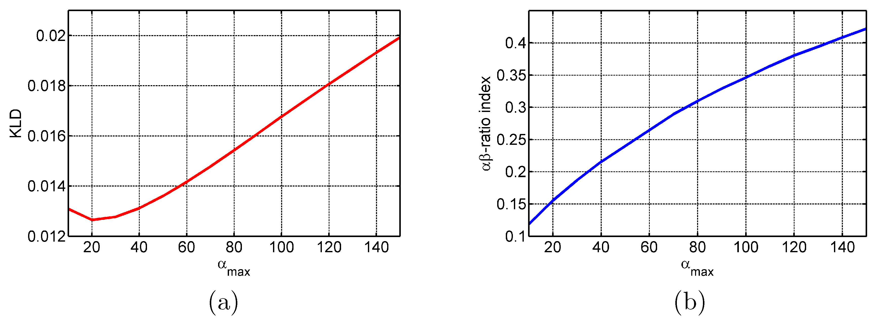
should be applied in the presence of edges. Moreover, the maximum value
is a specific input parameter that must be tuned for each test case in order to reach the highest performance of the filter.
In this framework, it is mandatory to estimate for each pixel the contextual information in order to use the optimal value of
. To this aim, we refer to the the Markovian Random Field theory (MRF). In particular, we adopt the Hyper-Parameter map
. This map is used to provide an index of spatial correlation between neighboring pixels [
21]. Hence, considering a local-central pixel
p and 8-connexity neighboring system
, the estimated hyper-parameter
of this pixel can be calculated in closed form as:
where
and
denote respectively the values of the central pixel
p and the neighboring pixel
q. Clearly,
and
are not a priori known (incomplete data problem), and they need to be estimated. For this reason, we used the filtered solutions, as will be specified in the following.
Based on Equation (
7), if a pixel belongs to a homogeneous area, then
will be small. On the contrary, if a pixel belongs to an edge,
will be large. Such a feature of
can be used to improve the efficiency of WF. The map provides the information about the probability that two pixels have the same values.
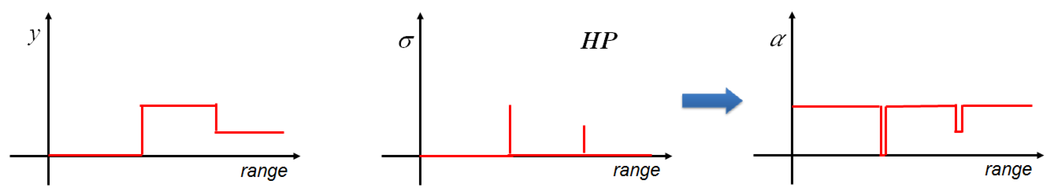
Once the hyper-parameter map is estimated, we define an
, which is simply an inversion of the
procedure. The
parameter is given by the following formula:
Figure 2 illustrates both
and
processes for a given image profile characterized by flat areas (homogeneous areas) and edges. It can be seen that
identifies those flat areas and those edges. From this, we can notice the process with the
parameter, which is presented as an inversion of
.
Hence, the provides for each pixel the optimal value of . In other words, it allows automatically selecting which is the best Wiener kernel to be applied for the specific pixel.
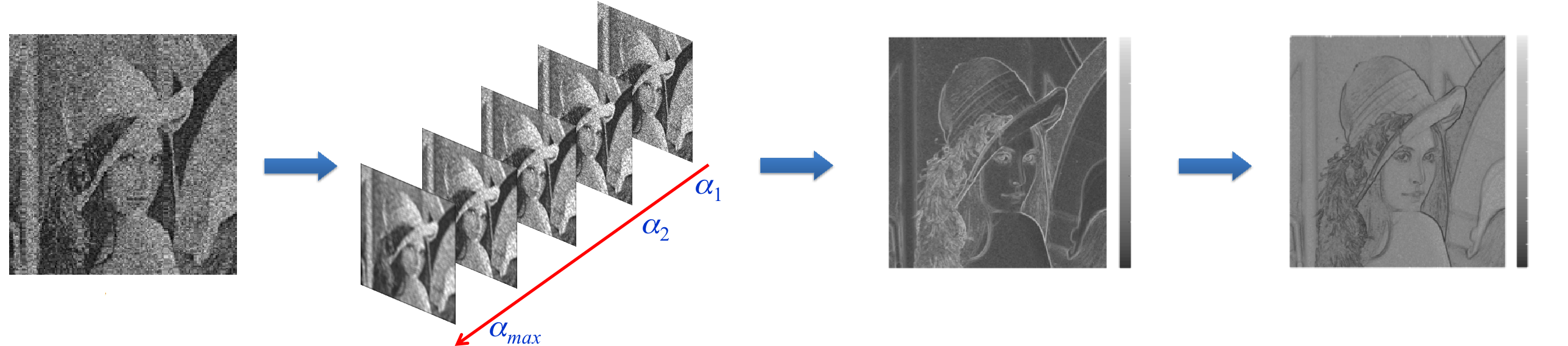
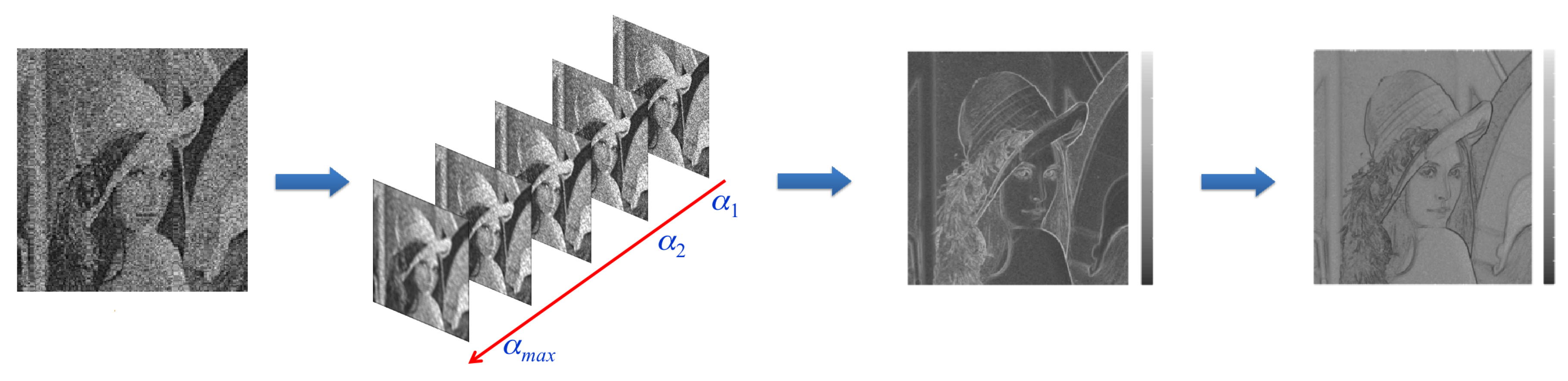
The processing steps of the proposed framework are illustrated in
Figure 3 by referring to the well-known Lena picture. The image is affected by speckle noise. The first step involves the homomorphic transformation of the noisy image. Then, in the second step, we apply the Wiener filtering based on the modified kernel
W′ using
K different parameters of vector
. Hence, this results in the generation of
K filtered images. For each obtained filtered image, we estimate the
using Equation (
7), and we merge them by averaging them in order to achieve a single
image. Then, the
is obtained by inverting the merged
output. Finally, we construct our final filtered output image by selecting each pixel from one of the
K solutions based on the
value presented in the
.
Algorithm 1 describes the steps to proceed with our proposed methodology, called the Enhanced Wiener Filter (EWF) framework [
22], starting from a noisy image and a specific input parameter, which is the maximum value of the
vector
. It should be noted that this latter must be tuned for each test case in order to reach the highest performance of the filter. The program was coded (
Supplementary Materials) in MATLAB R2018a [
23] environment, on an AMD Ryzen Threadripper 1950X 16-Core
-GHz processor with Linux Debian as the operating system. The GPU used in this paper was a GeForce GTX 1080 Ti work station characterized by 12 GB of memory and 3584 CUDA Cores.
As is clear from Algorithm 1, the methodology was designed using simple functions well suited for GPU processing such as FFT and matrix products. This helps in maintaining the high efficiency. The idea is to provide the GPU large amounts of data and ask it to perform relatively simple operations. Other implementations could be adopted, but at the cost of the processing time.
| Algorithm 1 Enhanced Wiener filter framework. |
- 1:
Apply the homomorphic transformation to the noisy image y (). - 2:
Compute the power spectrum Y′ of the degraded image y′. - 3:
Estimate the power density spectrum of the noise-free using the iterative procedure of [ 18]. - 4:
Create the vector. - 5:
forKdo - 6:
for each value , compute the correspondent defined in Equation ( 6). - 7:
Compute . - 8:
Apply the inverse Fourier transform function for the (). - 9:
Apply the exponential function to in order to obtain the filtered solutions in the initial temporal domain. - 10:
Estimate from based on Equation ( 7). - 11:
end for - 12:
Merge the obtained K hyper-parameter maps in a single . - 13:
Obtain the image presented in Equation ( 8). - 14:
Construct the final filtered output by selecting each pixel from one of the K solutions based on the value presented in .
|


