Abstract
As an active microwave sensor, synthetic aperture radar (SAR) has the characteristic of all-day and all-weather earth observation, which has become one of the most important means for high-resolution earth observation and global resource management. Ship detection in SAR images is also playing an increasingly important role in ocean observation and disaster relief. Nowadays, both traditional feature extraction methods and deep learning (DL) methods almost focus on improving ship detection accuracy, and the detection speed is neglected. However, the speed of SAR ship detection is extraordinarily significant, especially in real-time maritime rescue and emergency military decision-making. In order to solve this problem, this paper proposes a novel approach for high-speed ship detection in SAR images based on a grid convolutional neural network (G-CNN). This method improves the detection speed by meshing the input image, inspired by the basic thought of you only look once (YOLO), and using depthwise separable convolution. G-CNN is a brand new network structure proposed by us and it is mainly composed of a backbone convolutional neural network (B-CNN) and a detection convolutional neural network (D-CNN). First, SAR images to be detected are divided into grid cells and each grid cell is responsible for detection of specific ships. Then, the whole image is input into B-CNN to extract features. Finally, ship detection is completed in D-CNN under three scales. We experimented on an open SAR Ship Detection Dataset (SSDD) used by many other scholars and then validated the migration ability of G-CNN on two SAR images from RadarSat-1 and Gaofen-3. The experimental results show that the detection speed of our proposed method is faster than the existing other methods, such as faster-regions convolutional neural network (Faster R-CNN), single shot multi-box detector (SSD), and YOLO, under the same hardware environment with NVIDIA GTX1080 graphics processing unit (GPU) and the detection accuracy is kept within an acceptable range. Our proposed G-CNN ship detection system has great application values in real-time maritime disaster rescue and emergency military strategy formulation.
1. Introduction
As an active means of aerospace and aeronautical remote sensing, synthetic aperture radar based on microwave imaging technology has the characteristic of all-day and all-weather earth observation [1], which has a wide range of applications in environmental protection, disaster detection, ocean observation, resource exploration, and geological mapping [2]. The technology of ship target detection in synthetic aperture radar (SAR) images is of great significance for ocean surveillance and disaster relief. On the civil side, ship detection in designated sea areas and docks is conducive to shipwreck rescue and environmental protection; on the military side, traffic control and detection of other countries’ illegal ships can also be achieved. However, there are no rather mature theories and methods for target detection in SAR images up to now because the following obstacles still exist in the automatic recognition of ships in SAR images: (1) different from optical images, it is difficult to interpret SAR images intuitively; (2) due to the special imaging mechanism of SAR and the existence of speckle noise, subjective error in artificial interpretation is inevitable.
In 1978, the United States first acquired SAR surface ship targets from the Seasat-1 satellite, which opened up the exploration of ship detection technology in SAR images. Since the 1980s, more and more marine workers and governments have actively participated in the research of SAR ship detection algorithms [3,4,5,6,7,8,9,10,11,12,13,14,15,16,17,18,19,20,21,22,23,24,25,26,27,28,29,30,31,32,33,34,35,36,37,38,39,40,41,42,43]. According to our investigation, the methods of SAR ship detection are mainly divided into two categories—traditional methods and modern deep learning (DL) methods.
The remarkable characteristic of traditional methods is artificial feature extraction. The most basic method is to extract features of ships in SAR images, such as gray level, contrast ratio, texture, shape, and spatial relationship by the histogram of oriented gradient (HOG), local binary pattern (LBP), scale-invariant feature transform (SIFT), and Haar-like (Haar), to distinguish sea surface, dock, island, and so on. The representatives of these feature extraction methods are constant false alarm ratio (CFAR) and various improved CFAR detection algorithms. Among them, the most widely used ones are: (1) the two-parameter CFAR detection algorithm based on Gauss distribution proposed by Lincoln Laboratory [3]; (2) CFAR detection based on Weibull distribution by Kuttikkad [4]; and (3) optimal CFAR detection proposed by Anastassopoulos [5]. When using a traditional CFAR detection algorithm to detect target ships, it is necessary to fit the statistical distribution of background clutter according to pixels in SAR images, and then calculate the detection threshold to complete the ship detection. However, in practical application, the distribution of sea clutter is easily affected by sea wave and ocean current, which makes it difficult to select an appropriate statistical distribution to fit background clutter. In addition, due to a large number of calculations in solving the parameters of the above distribution, the processing speed of the algorithm cannot meet the actual needs. Another typical traditional method is template-based detection [6,7], which considers the characteristics of the target and background and estimates the backscattering characteristics of the small area around the target. However, the setting of template parameters comes from experience, lacks the necessary theoretical support, and its migration ability is weak. To sum up, these traditional ship detection methods will fall into a huge dilemma of feature engineering, which is not flexible and intelligent enough, and the speed of detection also is slow.
The remarkable characteristic of modern deep learning methods is automatic feature extraction [8,9]. Nowadays, more and more scholars are beginning to study the target detection algorithm based on data-driven and artificial intelligence (AI) methods [10,11,12,13,14,15,16,17,18,19,37,38,39,40,41,42,43]. A region-convolutional neural network (R-CNN) [10] applied DL to target detection for the first time. The traditional features (such as SIFT, HOG, etc.) are replaced by features extracted from deep convolution networks. However, the biggest disadvantage of R-CNN is the large number of calculations, resulting in very slow detection speed. Therefore, Fast R-CNN [11] was proposed to solve this problem by getting a region of interest (ROI) in feature maps. However, it still occupies a long time in the ROI extraction process. Ultimately, Faster R-CNN [12] emerged to make the detection speed faster by a region proposal network (RPN). From the emergence of these methods, we can conclude that speed is the primary factor, excepting accuracy.
However, nowadays, both traditional feature extraction methods and deep learning methods are almost focusing on improving ship detection accuracy [16,17,18,37,38,39,40,41,42], and the detection speed is neglected. Probably a simple explanation to this fact comes from the consideration of actual operational situations. Since the images which are dealt with are focused SAR images, the overall time required to get the images from the down-link station, focus, and then process them, in the fastest case cannot be below some minutes (most often, tens of minutes up to some hours). Consequently, adding to this computational budget a few milliseconds is in most cases a very minor concern. On the contrary, it is easy to realize that the issue of precision and accuracy is much more important to the end of efficient detection performances. However, the speed of ship detection is extraordinarily significant, especially in real-time maritime rescue and emergency military decision-making. Therefore, improving the speed of ship detection in SAR images is one of the key technologies in object detection nowadays.
In general, the practical application of ship detection in SAR images consists of two stages: (1) SAR image acquisition from aircraft or satellite; and (2) SAR image interpretation. In the first stage, the SAR imaging algorithm, such as range doppler (RD), chirp scaling (CS), back projection (BP), and so on, is mainly studied, which may take a long time to complete SAR imaging of an area. Once SAR images have been acquired, in the second stage, researchers in the field of image processing will interpret them to restore the real information of the area in a relatively short time compared with the first stage. In fact, current research [3,4,5,6,7,16,17,18,37,38,39,40,41,42,43] on image target detection are carried out on the premise that images have been obtained without considering the imaging process. For the second stage, it is meaningful and valuable to realize high-speed SAR ship detection in practical applications.
Therefore, in order to improve the detection speed of the second stage, this paper presents a high-speed ship detection method in SAR images based on a grid convolutional neural network (G-CNN). The inspiration for this method originates from you only look once (YOLO) [13,14,15]. G-CNN is mainly composed of a backbone convolutional neural network (B-CNN) and a detection convolutional neural network (D-CNN). First, SAR images are divided into grid cells and each grid cell is responsible for the detection of specific ships. Then, the whole image is input into B-CNN to extract features. Finally, ship detection is completed in D-CNN under three scales. This model based on mesh partition assigns ship detection tasks to each grid cell, which increases the detection speed. We experimented on an open SAR Ship Detection Dataset (SSDD) [16,17,18] to establish the ship detection model. In addition, in order to verify the applicability of G-CNN, we also detected ships in two SAR images from RadarSat-1 and Gaofen-3. The experimental results show that the detection speed of our proposed method is faster than most of the existing methods, such as the faster-regions convolutional neural network (Faster R-CNN), single shot multi-box detector (SSD) [19], and YOLO, under the same hardware environment with NVIDIA GTX1080 graphics processing unit (GPU), meanwhile the detection speed is almost maintained within an acceptable range. This method based on G-CNN has great application values in real-time maritime disaster rescue and emergency military strategy formulation.
The main contributions of our work are as follows:
- The detection speed of our proposed method is faster than the existing other methods.
- We established a brand new network structure G-CNN.
2. Methodology
2.1. Dataset
The first important factor of ship detection based on deep learning methods is to build a huge and representative dataset. Therefore, in order to fully consider the various conditions of ships in the ocean, we used the open SSDD [18] for experiments which has been used by many other scholars. Additionally, real ships have been correctly labeled by Li et al. [16,17,18].
There are 1160 SAR images in the SSDD from RadarSat-2, TerraSAR-X, and Sentinel-1 in Yantai, China and Visakhapatnam, India. The size of each image sample was about 500 × 500. The image annotation process is shown in Figure 1. LabelImg [20], software used for image annotation in the deep learning field, was applied to get parameters (x,y,w,h) of real ships where (x, y) was the coordinate of the upper left corner of the rectangular box, w is the width, and h is the height. For example, (x,y,w,h) of 0724.jpg is (152,141,332,220) in Figure 1c. Finally, all real ship information of the 1160 SAR images was obtained. More details can be found in reference [18].
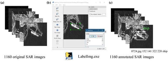
Figure 1.
Image annotation process. (a) 1160 original synthetic aperture radar (SAR) images in the SAR Ship Detection Dataset (SSDD); (b) LabelImg software; (c) 1160 annotated SAR images.
There are 2358 ships in the SSDD with different sizes and there are 2.03 ships in each image on average. There are at most 13 ships and at least one ship in an image. This dataset includes a variety of polarization modes, resolutions, and ship backgrounds, which can be used to verify the correctness of the proposed method. Detailed descriptions of the SSDD are shown in Table 1.

Table 1.
Detailed descriptions of the SSDD. H: Horizontal; V: Vertical.
Moreover, SAR images are formed by coherent processing of echoes from the continuous radar pulses, so SAR images are affected by speckle noise. In order to decrease negative effects by some bad samples with large speckle noise, we preprocessed these SAR images and constructed an enhanced SSDD named ESSDD by an adaptive refined lee filter [21]. We adopted the gradient operators corresponding to the 7 × 7 window to process images. Figure 2 is the detection template and edge direction window, including vertical, horizontal, 45°, and 135° directions.
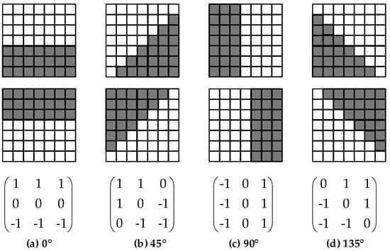
Figure 2.
The detection template and edge direction window of the refined lee filter. (a) 0°; (b) 45°; (c) 90°; (d) 135°.
The image before and after refined lee filtering is shown in Figure 3. From Figure 3, on the one hand, some speckles are restrained, and on the other hand, the basic features of ships are well preserved. Although image preprocessing can reduce the negative impact of noise, it may also degrade the performance of small ship detection. For example, as is shown in Figure 3d, the refined lee filter may smooth out some small ships from the original image. The effect of the size of the filter window on the detection performance will be discussed in Section 3.4.
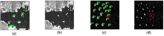
Figure 3.
Refined lee filter. (a,c) Two original images in the SSDD; (b,d) two filtered images in the ESSDD. The ground truth is marked in green and the red circle indicates that the ship may be miss-detected.
2.2. G-CNN
G-CNN is mainly composed of B-CNN and D-CNN as shown in Figure 4. First, the SAR image to be detected was resized to 416 × 416. Then the features of the ship were extracted by B-CNN in 1024 feature maps with a scale of 52 × 52. Finally, the output of B-CNN was connected to D-CNN to complete ship detection. B-CNN is the backbone of G-CNN, which is used to extract ship features. There are some network structures that can be used as the backbone of a target detector, such as visual geometry group-16 (VGG-16) [22], GoogLeNet [23], and so on. However, these network structures have more parameters and consume more computer memory, which will increase detection time. Therefore, we use a lightweight network MobileNet [24] to extract features. MobileNet is an efficient model for mobile and embedded devices. Based on streamlined architecture, MobileNet uses depthwise separable convolution (dw) to construct lightweight deep neural networks, which can greatly reduce the amounts of parameters and calculations.
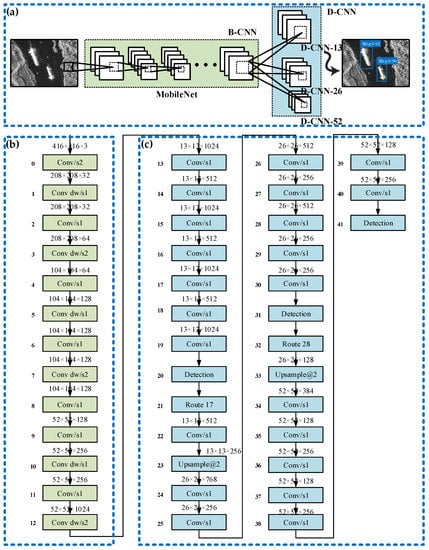
Figure 4.
The grid convolutional neural network (G-CNN) ship detection system. (a) Overall framework; (b) backbone convolutional neural network (B-CNN); (c) detection convolutional neural network (D-CNN).
D-CNN detects ships of different sizes at three scales 13 × 13, 26 × 26, and 52 × 52. We named these three detection scales as D-CNN-13, D-CNN-26, and D-CNN-52. D-CNN-13 was applied to the smallest 13 × 13 feature map (with the largest receptive field), which is suitable for detecting larger ships. D-CNN-26 was applied to the medium 26 × 26 feature map (medium receptive field), which is suitable for detecting medium-sized ships. D-CNN-52 was applied to the larger 52 × 52 feature map (smaller sensing field), which is suitable for detecting smaller objects.
Figure 5 is the diagram of depthwise separable convolution. Depthwise separable convolution divides the traditional convolution operation into two steps: (1) assuming that the original convolution is 3 × 3, depthwise separable convolution operates on the input M feature maps with 3 × 3 convolution kernels, and generates M results without summing them; (2) then, N convolution kernels of 1 × 1 are used to perform a normal convolution operation on the M results generated before, and the sum is used to generate N results. Compared with VGG-16, the accuracy of MobileNet is slightly lower, but better than GoogLeNet. MobileNet reduces the amount of computation and parameters by two times which can achieve high speed and efficient ship detection [24].
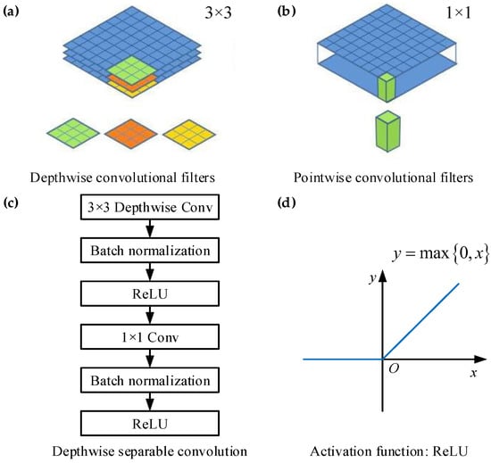
Figure 5.
Depthwise separable convolution. (a) Depthwise convolutional filters; (b) pointwise convolutional filters; (c) depthwise separable convolution; (d) activation function: Rectified linear unit (ReLU).
Batch normalization (BN) in Figure 5c can accelerate the convergence speed of the network [25], whose function is to normalize the mean and variance of input data x. Algorithm 1 [25] of batch normalization transform is as follows. More details can be found in reference [25].
| Algorithm 1 [25]. Batch Normalizing Transform, applied to activation x over a batch. |
| Input: Values of x over a batch: Parameters to be learned: |
| Output: |
Rectified linear unit (ReLU) [26] in Figure 5c is the activation function whose function image is shown in Figure 5d. ReLU can not only overcome gradient disappearance but also speed up training, which has been widely used in the field of deep learning.
ReLU is defined by:
2.3. Model
Figure 6 is the general process of ship detection based on deep learning. As is shown in Figure 6, a dataset was needed first to build a detection model in the deep learning field.
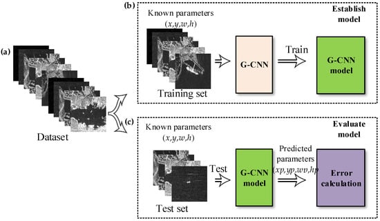
Figure 6.
General process of ship detection based on deep learning. (a) Dataset; (b) establish model; (c) evaluate model.
Moreover, the dataset must have been correctly labeled. Additionally, the dataset was divided into: (1) a training set which was used to establish a detection model; (2) a test set which was used to evaluate the detection model. According to the parameters of the known real ships in the training set, G-CNN fits these parameters by iteration many times to minimize the error. Finally, the ship detection model was obtained by training. Afterwards, the test set was used to evaluate the performance of the detection model. In other words, by calculating the error between the predicted parameters (xp,yp,wp,hp) and the known parameters (x,y,w,h).
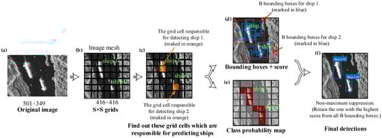
Figure 7.
G-CNN ship detection model. (a) Original image; (b) S × S grids; (c) find out these grid cells which are responsible for predicting ships; (d) bounding boxes + score; (e) class probability map; (f) final detections.
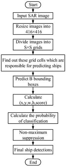
Figure 8.
G-CNN ship detection flow chart.
The entire algorithm of ship detection is as follows.
Step 1: Input SAR images.
Step 2: Resize images into 416 × 416.
The size of each image sample in the SSDD is about 500 × 500. However, these 1160 SAR images are not all the same size, such as 416 × 323, 467 × 391, 480 × 481, 498 × 377, 501 × 349, and so on. In the field of deep learning, every pixel of an image is a feature. For an n × n image, its feature vector is (x11, x12, …, x1n, x21, x22, …, x2n, …, xn1, xn2, …, xnn) whose dimension is n2. Therefore, in order to obtain the feature vector of images with the same dimension, we resized images into 416 × 416 by image resampling as is shown in Figure 7a,b. In particular, G-CNN has two down-sampling steps and each sampling step is 2, the maximum step of the network (layer input size divided by output) is 22 = 4. As a result, images whose size just satisfies a multiple of 4 all can be input into the network besides 416 × 416. The following research in Section 3.3 shows that images with a 416 × 416 size have higher accuracy than others, so we choose 416 × 416 images as the input of G-CNN.
Step 3: Divide images into S × S grids.
Our G-CNN system divides the SAR image into S × S grid cells, like a mesh structure as shown in Figure 7b. We also set S = 7 as a good tradeoff between speed and accuracy. More details can be found in reference [13].
Step 4: Find out these grid cells which are responsible for predicting ships.
As is shown in Figure 7c, the trained detection model can automatically find the center of a ship. If the center of a ship falls into a grid cell, that grid cell is responsible for detecting that ship. If a grid cell contains a ship, then Pr(ship) = 1, else Pr(ship) = 0.
Step 5: Predict B bounding boxes.
Each grid cell predicts B bounding boxes and confidence scores for those boxes. The value of B can be dynamically adjusted to achieve optimal performance. As is shown in Figure 7d, we set B = 9 as a good tradeoff between speed and accuracy, which means that G-CNN produces 9 predicted bounding boxes (marked in blue) for ship 1 and ship 2, respectively. In addition, the size of these 9 boundary boxes are different because they are predicted in different layers.
Step 6: Calculate predictive parameters (x,y,w,h,score).
Each bounding box contains five predictive parameters (x,y,w,h,score).
The score is defined by:
where IoU is intersection over union.
Intersection over union (IoU) is defined by:
where G is the actual position of ships (Ground truth bounding box), and P is the predicted position (Predicted bounding box).
IoU is used to measure the correlation between reality and prediction. Obviously, the larger the value is, the better detection performance is. When IoU = 1, the detection performance is the best, but generally speaking, it has been a very good result when IoU > 0.5 in the actual detection.
Therefore, according to the definitions of Pr(ship) and IoU, the value range of score is [0,1], which reflects how confident the model is that the box contains a ship and also how accurate it thinks the box is that it predicts.
Step 7: Calculate the probability of classification.
As is shown in Figure 7e, in the field of deep learning, generally, after the target is detected, the detection system also needs to classify the target such as bird, cat, dog, and so on in the PASCAL VOC dataset [27]. Because we only need to detect one type of target in the SSDD, the target is recognized as a ship directly once detected. In short, conditional probability Pr(ship|target) = Pr(ship).
Step 8: Non-maximum suppression [28].
For each ship, G-CNN generates 9 predicted boxes, the box with the highest score is retained, and the rest is suppressed.
Step 9: Final ship detection results.
2.4. Anchor Box
The concept of the anchor box was first proposed in Faster R-CNN by Ren [12], which is widely used in other excellent target recognition models afterward, such as YOLO and SSD. An anchor box is proposed to solve the shortcoming that a grid cell detects only one ship.
For example, for the case in Figure 9b, the two ships (marked by blue circles) are situated in the same grid cell G. From Section 2.3, only the highest score prediction box was retained (non-maximum suppression) which means that only one ship could be detected at last. Obviously, if ships are very small and densely distributed, they may appear in the same grid cell, and as a result, many ships will be missed, which will inevitably reduce the accuracy of detection. To solve this problem, we can set up two anchor boxes shown in Figure 9c. According to the previous method, the detection tasks of ship 1 and ship 2 are assigned to the grid cell G. Now, we further assigned the detection task of ship 1 to anchor box 1 and that of ship 2 to anchor box 2, according to the center of the ship. Therefore, the grid cell G can detect two ships at the same time. Certainly, this problem can also be solved by dividing the meshes more finely (increase the value of S) but the method of the anchor box is more effective [12].
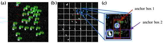
Figure 9.
Anchor box. (a) Ground truth; (b) image mesh; (c) the grid cell responsible for predicting ships.
In the G-CNN ship detection system, we set 9 anchor boxes which can detect 9 ships in the same grid cell at the same time. The size of the anchor box can be obtained by the K-means algorithm. If we use standard K-means with Euclidean distance, larger boxes generate more error than smaller boxes. However, what we really want are priors that lead to good IoU scores, which are independent of the size of the box. Thus, for our distance metric, we use [14]:
The cluster centroids were significantly different than hand-picked anchor boxes. There were fewer short, wide boxes and taller, thin boxes. The results of K-means is shown in Figure 10 and the size of each anchor box for three scales are shown in Table 2. More details can be found in reference [14].
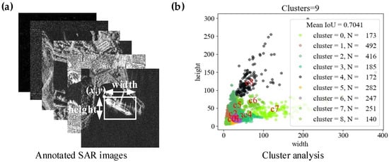
Figure 10.
The results of K-means. (a) Annotated SAR images; (b) cluster analysis.
Table 2.
Anchor boxes of D-CNN-13, D-CNN-26, and D-CNN-52.
2.5. Evaluation Indicator
Recall is defined by:
Precision is defined by:
In SAR ship detection, TP means that ships are correctly detected, FP means miss-detection, and FN means false alarm.
Empirical studies of detection performance have shown a tendency for precision to decline as recall increases [29]. Obviously, we need to use recall and precision to measure the performance of ship detection. We can also use another one parameter to describe the performance of target detection, which is mAP (mean average precision).
Mean average precision (mAP) is defined by:
where P is precision, R is recall, P(R) is a function with R as an independent variable and P as a dependent variable. Mean average precision (mAP) measures the performance of object detection for several classes such as bird, cat, dog, and so on in the PASCAL VOC dataset [27]. If there is only one class to detect, such as ship in the SSDD, mAP can be simplified to AP (average precision) [30]. In the following description, we will use AP to measure the performance of our detector.
3. Experiments and Results
Our experimental platform was a personal computer with Intel(R) i7-8700 CPU @3.20GHz processor, 16G memory, and NVIDIA GTX1080 graphics card with 8G memory.
3.1. Establishment of Training Model
We randomly divided the dataset into a training set, validation set, and test set according to the ratio of 7:2:1, where the validation set was used to adjust the model’s hyperparameters to avoid over-fitting [9]. Then, the G-CNN network was established based on the Keras framework, a compact and easy-to-learn high-level Python (a programming language similar to MATLAB) library for deep learning [31]. The adaptive moment estimation (ADAM) [32] algorithm similar to stochastic gradient descent (SGD) [33] was used to update the weights and biases in the network, with the advantages of efficient calculation and less memory. Because of the memory limitation of the graphics card, we set batch size = 8 which means that every 8 training samples were sent into the network to complete parameter updating. The batch is a part of the training data sent into the network each time, and batch size is the number of training samples in each batch [34]. In the field of deep learning, all training data can be sent to the network for parameter updating once, but this method reduces the convergence speed of the algorithm [34], so we can only send partial training samples at a time to perform parameter iteration. We set the learning rate of the first 100 iterations to 0.001. In addition, we also set up an additional mechanism to automatically adjust the learning rate, by which the learning rate will automatically be reduced when the loss of the verification set does not decrease any more beyond three times. To avoid over-fitting, we limited the capacity of the network by early stopping [35]. In this way, the training will be forcibly suspended ultimately, if the performance of the model on the verification set starts to decline continuously.
3.2. Feature Maps
In the field of deep learning, features of the ship are extracted automatically by CNN without manual involvement. There are fewer reports visualizing the feature maps [10,11,12,13,14,15,16,17,18,19,20] because the detection system based on deep learning is a black-box model. In other words, the feature extracted by the convolution neural network is abstract and difficult to explain [8]. Therefore, in order to fill the vacancy, we tried to visualize the trained model to explain the process of feature extraction in our proposed G-CNN. From Figure 4b in Section 2.2, the outputs of 2-layer were 208 × 208 × 64 feature maps, where 208 × 208 was the size of the feature map and 64 was the number of feature maps. Additionally, the feature maps were 104 × 104 × 128 for 6-layer and 52 × 52 × 256 for 10-layer. We choose two feature maps from each layer for visualization, respectively, shown in Figure 11b–d.
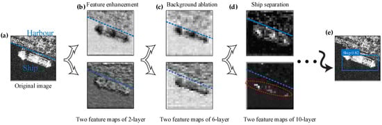
Figure 11.
The process of feature extraction. (a) Origin image; (b) two feature maps of 2-layer; (c) two feature maps of 6-layer; (d) two feature maps of 10-layer; (e) detection results.
From Figure 11b–d, the features of the ship were enhanced such as the contrast, edge, and shape in 2-layer. Additionally, in 6-layer, the background begins to fade, and the ship’s features were retained. Finally, the harbor disappears, and the ship is completely separated from the harbor in 10-layer. With the deepening of layers, the extracted ship features will become more and more abstract, which can extract potential features and make it easier to detect ships. More details can be found in reference [36].
3.3. Results of G-CNN
We trained on the SSDD and ESSDD, and finally got the ship detection model. Then we carried out actual ship detection on the test set. We set score = 0.3 (score∈[0,1]) as the detection threshold, which means that if the probability of a bounding box containing a ship is greater than or equal to 30%, it is retained. The value of the score needs to be set reasonably as a good tradeoff between false alarm and miss-detection according to the actual situation. We also set IoU = 0.5 as another detection threshold.
In addition, it should be noted that image preprocessing (32 s per image), which will certainly increase training time, was to establish more accurate models avoiding the negative impact of bad samples in the training process. However, when actual ship detection was carried out in the test process, images were not preprocessed, so the detection process does not contain the time of image preprocessing as is shown in Figure 12. Thus:
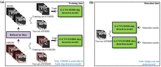
Figure 12.
Explanation of training time and detection time. (a) Training time; (b) detection time.
There were 183 real ships in the test set. The ship test results between the SSDD and ESSDD are shown in Table 3. The precision and recall (P-R) curve of SSDD and ESSDD is shown in Figure 13. From Table 3, our enhanced dataset ESSDD by refined lee filter has better performance than the origin dataset SSDD. The AP of ship detection on ESSDD reaches 90.16%, which is an acceptable range in practical applications. The test time per image on the SSDD and ESSDD is about 21 ms.
Table 3.
The ship test results of SSDD and ESSDD. AP: average precision.
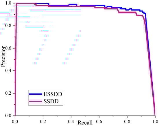
Figure 13.
The P-R curve of SSDD and ESSDD. P: precision; R: recall.
The ship detection results of some samples are shown in Figure 14. From Figure 14c, G-CNN mistook the coast for a ship (marked in yellow). One possible reason may be the high similarity between the coast and the ship. From Figure 14g, real ships are so small and densely distributed and one ship was miss-detected (marked in red). However, for these eight backgrounds, the G-CNN ship detection system can detect almost all ground truth ships, which fully confirms the feasibility of our proposed method.
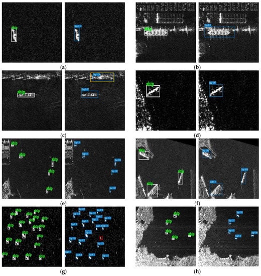
Figure 14.
The ship detection results of some samples. (a–h) Various backgrounds. The ground truth is marked in green, the predicted boxes are marked in blue, miss-detection is marked in red, and false alarm is marked in yellow.
In addition, we compared the effects of different B-CNNs on detection accuracy and time shown in Figure 15. From Figure 15, the AP of VGG-16 and GoogLeNet is greater than MobileNet. However, the AP gap between them is not rather big. Meanwhile, MobileNet takes significantly less time than VGG-16 and GoogLeNet, which fully verifies that MobileNet is a lightweight network authentically and can be used to reduce the detection time of ships.
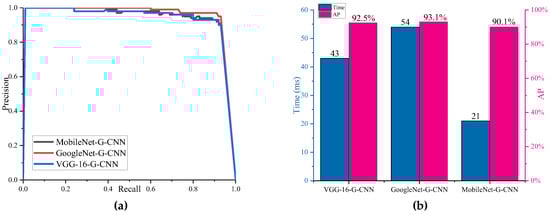
Figure 15.
Different B-CNNs. (a) P-R curve; (b) AP and detection time.
In order to further improve the detection efficiency, we also tried to use only one scale or two scales to detect ships. The AP and detection time of different scales are shown in Table 4. From Table 4, when only one scale was used, it took the least time but the AP was too poor to meet the practical application requirements. Additionally, when two scales were used, AP had been improved meanwhile the detection time had increased. However, if we used three scales, the accuracy was greatly improved and the detection time was acceptable. Therefore, these three scales together constitute D-CNN to improve the detection accuracy of ships in our G-CNN ship detection system.
Table 4.
The AP and detection time of different scales.
Finally, we also studied the influence of different input scale images on the test results. We resized SAR images to be detected to three input sizes 320 × 320, 416 × 416, and 608 × 608. We named these G-CNNs as G-CNN-320, G-CNN-416, and G-CNN-608, separately. The AP and detection time of ship detection are shown in Figure 16. From Figure 16, we can find that the smaller the size of the image input into the network is, the less the detection time will be. G-CNN-416 has the highest detection accuracy, which may be related to the original size of the image in the dataset. Therefore, we chose G-CNN-416 as the final ship detection model.
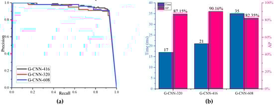
Figure 16.
Input of different sized images. (a) P-R curve; (b) AP and detection time.
3.4. Results of Different Methods
The ship detection results for the same dataset are shown in Figure 17. From Figure 17, these four methods have excellent performance for those simple samples and G-CNN has almost a similar detection accuracy compared to others. In addition, from the last sample in Figure 17, the detection performance of G-CNN may be lower than that of Faster R-CNN and SSD for ships with smaller size and dense distribution. One possible reason is the role of a pre-processing refined lee filter. On the one hand, a refined lee filter can reduce the negative impact of high noise, but on the other hand, it may also smooth out some small ships.
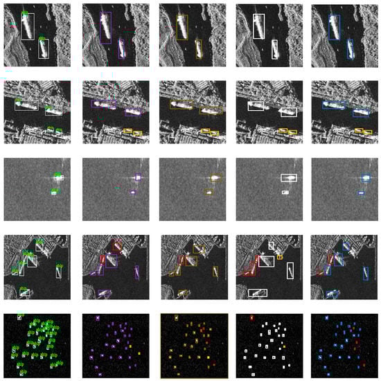
Figure 17.
The ship detection results of different methods. (a) Ground truth; (b) faster-regions convolutional neural network (Faster R-CNN); (c) you only look once (YOLO); (d) single shot multi-box detector (SSD); (e) G-CNN. The miss-detection is marked in red and the false alarm is marked in yellow.
Therefore, we also studied the effect of a pre-processing refined lee filter on high-noise samples and small ship samples as is shown in Figure 18. From Figure 18, the detection performance of G-CNN with a refined lee filter for high-noise samples was superior to that of G-CNN without a refined lee filter. In the second high-noise image, a ship with distinct features was missed meanwhile a false alarm appeared. The false alarm rate of G-CNN with a refined lee filter was less than that of G-CNN without a refined lee filter for those small ship images. Finally, we still chose G-CNN with a refined lee filter as the ship detection model to improve accuracy (from 87.48% to 90.16% shown in Table 3) because the number of high-noise images (19.91% of 1160) is more than that of small ship images (2.8% of 1160). We also tried to adjust the size of the filter window, but the improvement of detection performance was not obvious for the whole dataset. In fact, small target detection has become an important branch of deep learning object detection, which is being studied by many other scholars. Given that the primary task of this paper was to improve the detection speed, we have not carried out a detailed study of small target detection.
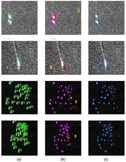
Figure 18.
The effect of a pre-processing refined lee filter on high noise samples and small ship samples. (a) Ground truth; (b) G-CNN without refined lee filter; (c) G-CNN with refined lee filter. The miss-detection is marked in red and the false alarm is marked in yellow.
In addition, we also studied the impact of models built from the SSDD and ESSDD on AP by different methods, respectively. From Equation (8), since the detection time between SSDD and ESSDD was equal, we omitted the comparison of time. The results are shown in Figure 19. From Figure 19a, although a refined lee filter may have a negative impact on small ship detection, the overall performance of the detection model based on ESSDD is better than that of SSDD, coming from a small proportion of small ship samples (2.8%) in the whole dataset. From Figure 19b,c, our G-CNN detection accuracy was slightly lower than other methods, but the gap was small. More importantly, the G-CNN ship detection system can sacrifice a little precision to increase the detection speed several times, which is a great improvement. More details will be discussed in Section 4.2.
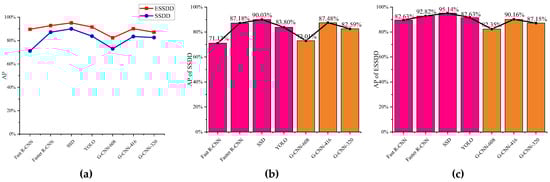
Figure 19.
The impact of models built from the SSDD and ESSDD on AP by different methods. (a) AP of the SSDD and ESSDD; (b) AP of the SSDD; (c) AP of the ESSDD.
3.5. Actual Ship Detection for RadarSat-1 and Gaofen-3
The model of our G-CNN ship detection system was obtained based on the training of the SSDD and ESSDD. In order to verify the wide practicability of the G-CNN ship detection system, we validated two SAR images from RadarSat-1 and Gaofen-3. Detailed descriptions of these two SAR images are shown in Table 5.
Table 5.
Detailed descriptions of two SAR images from RadarSat-1 and Gaofen-3.
We divided the two big SAR images into 64 sub-images, and then we resized the 64 sub-images into 416 × 416. Lastly, these 64 sub-images were inputted into the G-CNN ship detection system. Because the acquisition time of the two SAR images was different from the current time, we drew support from Google Earth to identify some islands and docks whose locations may not change with time, by human eye observation. Additionally, the Association for Information Systems (AIS) system was used to judge the possible berthing position of ships and exclude positions where the ships were impossible to appear. By the above two means, we could not get the real ship information of these two SAR images strictly but tried to get the information relatively close to the real situation. In fact, because Google Earth images change as time goes on, there were certain difficulties making Google Earth images acquire a close temporal connection with the SAR images. The detection results are shown in Table 6 and Figure 20. From the test results, the performance of Image 2 was inferior to that of Image 1, because the ships in Image 2 were too dense and the background was more complex. In short, most ships were accurately detected which shows that our G-CNN ship detection system has good migration ability and practical value.
Table 6.
The ship detection results of RadarSat-1 and Gaofen-3. TP: ships are correctly detected; FN: false alarm; FP: miss-detection.
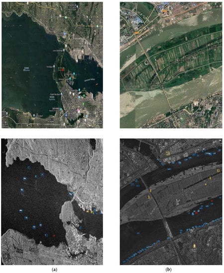
Figure 20.
The ship detection results of RadarSat-1 and Gaofen-3. (a) Image 1; (b) Image 2. Correct ship detection is marked in blue, the miss-detection is marked in red, and the false alarm is marked in yellow.
4. Discussion
In Section 3, we emphatically verified the effectiveness and practicability of the proposed method. In this section, we will focus on introducing the detection speed of our G-CNN system.
4.1. Complexity Analysis
The other methods, such as Faster R-CNN, SSD, and YOLO, adopt standard convolution to complete image feature extraction. Therefore, in order to reduce the amount of calculation and improve the detection speed, depthwise separable convolution [24] is used in G-CNN. The comparison of the computational complexity of standard convolution and depthwise separable convolution is shown in Figure 21.
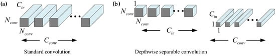
Figure 21.
Comparison of standard convolution and depthwise separable convolution. (a) Standard convolution; (b) depthwise separable convolution.
Assume that the size of the input image is Nin × Nin. The number of channels is Cin. The size of the convolution core is Nconv × Nconv × Cin and the number is Cconv. Additionally, the size of output feature maps is Cconv × Nin × Nin, so the amount of standard convolution required calculation (Amountstandard) is:
When we use depthwise separable convolution, the amount of required calculation (Amountdepthwise) is:
Thus, we get the ratio of the computational complexity of two convolutions:
From Equation (11), depthwise separable convolution effectively reduces the amount of computation compared to standard convolution under the same computational effects (ratio < 1). Additionally, their calculation ratio is only related to the number and size of used convolution kernels.
The time complexity of standard convolution is as follows:
where M is the edge length of the output feature map for each convolution kernel, K is the edge length of each convolution kernel, Cin is the channel number for each convolution kernel (number of input channels), and Cout is the number of convolution kernels in current convolution layer (number of output channels).
The time complexity of depthwise separable convolution is as follows:
From Equations (12) and (13), depthwise separable convolution used in G-CNN essentially transforms continuous multiplication into continuous addition which reduces the redundancy of the model. Therefore, the number of operations is less, and the number of parameters is also reduced. Ultimately, the speed of ship detection in SAR images can be significantly improved.
4.2. Detection Time
We used other methods, such as Faster R-CNN, SSD, and YOLO, for comparison, under the same hardware environment with NVIDIA GTX1080 GPU. The detection time of our proposed G-CNN method is the least as shown in Figure 22. Our G-CNN ship detection system needs 21 ms to complete the detection of an image with a 416 × 416 size. If we need faster speed, we can adopt G-CNN-320 but the accuracy will reduce a little. Therefore, our method achieves high-speed SAR ship detection, really and truly. Moreover, from Figure 19 and Figure 22, our G-CNN ship detection system can sacrifice a little precision to increase the detection speed several times, which is a great improvement.
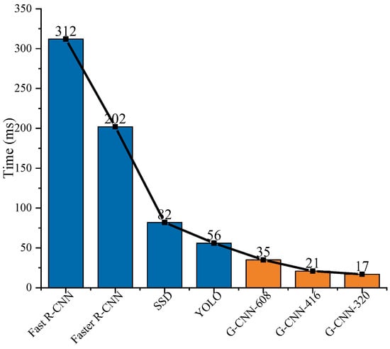
Figure 22.
The ship detection time of different approaches.
Our G-CNN ship detection system can save tens or even hundreds of milliseconds compared with the other methods. The increase of speed is not obvious enough in terms of two stages of practical application of SAR ship detection, which is rather small with respect to the typical times required for complete processing of a SAR image, from sensing by the satellite sensor to ship identification. However, it is remarkable for only the second stage without regard to the process from satellite acquisition to imaging (the first stage). In general, millisecond level time saving is meaningful and valuable in the field of image processing. For example, G-CNN only needs 24.36 s to detect 1160 SAR images in total while Fast R-CNN takes 6.032 min, which is a significant improvement for an ordinary computer in the field of image recognition. In fact, some other methods, such as Fast R-CNN, Faster R-CNN, YOLO, SSD, and so on, also only consider the second stage from 312 ms to 56 ms shown in Figure 22. In addition, under the condition of the same detection speed, our G-CNN can use hardware with slightly poor performance, which will bring greater economic benefits.
Finally, we compared the references with a similar hardware environment with NVIDIA GTX1080 graphics card and the contrasting results of detection time are shown in Figure 23. From Figure 23, the detection speed of our G-CNN ship detection system was faster than the methods in most references. When we chose G-CNN-416, the detection speed was the fastest. In particular, the detection time of traditional feature extraction methods reached the second level, so we ignored their comparison. Moreover, it should be noted that reference [43] only takes 11 ms to complete the detection of an image. However, the graphics card they use is NVIDIA TITAN X, whose performance is better than NVIDIA GTX1080 we used, so it was not convenient to make a reasonable comparison.
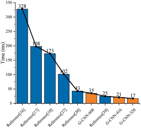
Figure 23.
The ship detection time of different references.
5. Conclusions
Aiming at the situation that the speed of SAR ship detection is neglected at present, we proposed a novel approach for high-speed ship detection in SAR images based on G-CNN in this paper. This G-CNN ship detection system mainly consists of B-CNN and D-CNN. The network structure of B-CNN comes from MobileNet, which is used to extract the ship’s features. Additionally, we visualized the process of feature extraction which fills the vacancy in the work of other scholars. D-CNN completes SAR ship detection under three scales D-CNN-13, D-CNN-26, and D-CNN-52. We confirmed the validity of the proposed method on a public SSDD and then constructed an enhanced ESSDD through refined lee filtering to improve accuracy. The ship detection accuracy of our G-CNN ship detection system is maintained within an acceptable range for practical application. More importantly, our method is superior to other existing methods in ship detection speed, under a similar hardware environment with NVIDIA GTX1080 GPU. Our proposed method realizes the high-speed ship detection in SAR images with only 21 ms detection time per image, authentically. The proposed method can satisfy real-time SAR ship detection and is of great value in maritime distress rescue and emergency military strategy formulation.
Future works: Our G-CNN SAR ship detection system has a slightly lower performance for small and dense ships. Therefore, further improvement is needed to solve this problem.
Author Contributions
T.Z. conducted experiments and paper writing. X.Z. provided technical guidance and paper review.
Funding
This work was supported in part by the National Natural Science Foundation of China under Grants 61571099 and in part by the National Key R&D Program of China under Grant 2017YFB0502700.
Acknowledgments
We thank all reviewers for their comments towards improving our manuscript. We thank Canadian Space Agency (CSA) and China National Space Administration (CNSA) for providing SAR images. The authors would also like to thank Durga Kumar for his linguistic assistance during the preparation of this manuscript.
Conflicts of Interest
The authors declare no conflict of interest.
References
- Schwartz, G.; Alvarez, M.; Varfis, A.; Kourti, N. Elimination of false positives in vessels detection and identification by remote sensing. In Proceedings of the 2002 IEEE International Geoscience and Remote Sensing Symposium (IGARSS), Toronto, ON, Canada, 24–28 June 2002; pp. 116–118. [Google Scholar]
- Sempreviva, A.M.; Barthelmie, R.J.; Pryor, S.C. Review of Methodologies for Offshore Wind Resource Assessment in European Seas. Surv. Geophys. 2008, 29, 471–497. [Google Scholar] [CrossRef]
- Raj, N.; Sethunadh, R.; Aparna, P.R. Object detection in SAR image based on bandlet transform. J. Vis. Commun. Image Represent. 2016, 40, 376–383. [Google Scholar] [CrossRef]
- Kuttikkad, S.; Chellappa, R. Non-gaussian CFAR techniques for target detection in high resolution SAR images. In Proceedings of the IEEE International Conference on Image Processing (ICIP-94.), Austin, TX, USA, 13–16 November 1994. [Google Scholar]
- Anastassopoulos, V.; Lampropoulos, G.A. Optimal CFAR detection in Weibull clutter. IEEE Trans. Aerosp. Electron. Syst. 1995, 31, 52–64. [Google Scholar] [CrossRef]
- Zhu, J.; Qiu, X.; Pan, Z.; Zhang, Y.; Lei, B. Projection Shape Template-Based Ship Target Recognition in TerraSAR-X Images. IEEE Geosci. Remote Sens. Lett. 2017, 14, 222–226. [Google Scholar] [CrossRef]
- Wang, C.; Bi, F.; Chen, L.; Chen, J. A novel threshold template algorithm for ship detection in high-resolution SAR images. In Proceedings of the IEEE Geoscience and Remote Sensing Symposium, Beijing, China, 10–15 July 2016. [Google Scholar]
- Lecun, Y.; Bengio, Y.; Hinton, G. Deep learning. Nature 2015, 521, 436. [Google Scholar] [CrossRef] [PubMed]
- Krizhevsky, A.; Sutskever, I.; Hinton, G.E. ImageNet classification with deep convolutional neural networks. In Proceedings of the International Conference on Neural Information Processing Systems, Lake Tahoe, NV, USA, 3–6 December 2012. [Google Scholar]
- Girshick, R.; Donahue, J.; Darrell, T.; Malik, J. Rich Feature Hierarchies for Accurate Object Detection and Semantic Segmentation. In Proceedings of the 2014 IEEE Conference on Computer Vision and Pattern Recognition, Columbus, OH, USA, 23–28 June 2014; pp. 580–587. [Google Scholar]
- Girshick, R. Fast R-CNN. In Proceedings of the 2015 IEEE International Conference on Computer Vision (ICCV), Santiago, Chile, 7–13 December 2015; pp. 1440–1448. [Google Scholar]
- Ren, S.; He, K.; Girshick, R.; Sun, J. Faster R-CNN: Towards Real-Time Object Detection with Region Proposal Networks. IEEE Trans. Pattern Anal. Mach. Intell. 2017, 39, 1137–1149. [Google Scholar] [CrossRef] [PubMed]
- Redmon, J.; Divvala, S.; Girshick, R.; Farhadi, A. You Only Look Once: Unified, Real-Time Object Detection. In Proceedings of the 2016 IEEE Conference on Computer Vision and Pattern Recognition (CVPR), Las Vegas, NV, USA, 27–30 June 2016. [Google Scholar]
- Redmon, J.; Farhadi, A. YOLO9000: Better, Faster, Stronger. In Proceedings of the 2017 IEEE Conference on Computer Vision and Pattern Recognition (CVPR), Honolulu, HI, USA, 21–26 July 2017; pp. 6517–6525. [Google Scholar]
- Joseph, R.; Ali, F. YOLOv3: An Incremental Improvement. Available online: https://pjreddie.com/media/files/papers/YOLOv3.pdf (accessed on 1 April 2019).
- Li, J.; Qu, C.; Peng, S.; Jiang, Y. Ship Detection in SAR images Based on Generative Adversarial Network and Online Hard Examples Mining. J. Electron. Inf. Technol. 2019, 41, 143–149. [Google Scholar]
- Li, J.; Qu, C.; Peng, S.; Deng, B. Ship detection in SAR images based on convolutional neural network. Syst. Eng. Electron. 2018, 40, 1953–1959. [Google Scholar]
- Li, J.; Qu, C.; Shao, J. Ship detection in SAR images based on an improved faster R-CNN. In Proceedings of the SAR Big Data Era: Models, Methods, Applications (BIGSARDATA), Beijing, China, 13–14 November 2017. [Google Scholar]
- Liu, W.; Anguelov, D.; Erhan, D.; Szegedy, C.; Reed, S.; Fu, C.Y.; Berg, A.C. SSD: Single Shot MultiBox Detector. In Proceedings of the European Conference on Computer Vision, Amsterdam, The Netherlands, 11–14 October 2016; pp. 21–37. [Google Scholar]
- Github. Available online: https://github.com/tzutalin/labelImg (accessed on 7 May 2019).
- Lopes, A.; Touzi, R.; Nezry, E. Adaptive speckle filters and scene heterogeneity. IEEE Trans. Geosci. Remote Sens. 1990, 28, 992–1000. [Google Scholar] [CrossRef]
- Simonyan, K.; Zisserman, A. Very Deep Convolutional Networks for Large-Scale Image Recongnition. Available online: http://vc.cs.nthu.edu.tw/home/paper/codfiles/melu/201604250548/VGG.pdf (accessed on 1 April 2019).
- Szegedy, C.; Liu, W.; Jia, Y.; Sermanet, P.; Reed, S.; Anguelov, D.; Erhan, D.; Vanhoucke, V.; Rabinovich, A. Going Deeper with Convolutions. In Proceedings of the 2015 IEEE Conference on Computer Vision and Pattern Recognition (CVPR), Boston, MA, USA, 7–12 June 2015. [Google Scholar]
- Howard, A.G.; Zhu, M.; Chen, B.; Kalenichenko, D.; Wang, W.; Weyand, T.; Andreetto, M.; Adam, H. MobileNets: Efficient Convolutional Neural Networks for Mobile Vision Applications. 2017. Available online: https://arxiv.org/pdf/1704.04861.pdf (accessed on 1 April 2019).
- Ioffe, S.; Szegedy, C. Batch normalization: Accelerating deep network training by reducing internal covariate shift. In Proceedings of the International Conference on Machine Learning, Lille, France, 6–11 July 2015. [Google Scholar]
- Jarrett, K.; Kavukcuoglu, K.; LeCun, Y. What is the best multi-stage architecture for object recognition? In Proceedings of the 2009 IEEE 12th International Conference on Computer Vision, Kyoto, Japan, 29 September–2 October 2009; pp. 2146–2153. [Google Scholar]
- Everingham, M.; Eslami, S.A.; Van Gool, L.; Williams, C.K.; Winn, J.; Zisserman, A. The Pascal Visual Object Classes Challenge: A Retrospective. Int. J. Comput. Vis. 2015, 111, 98–136. [Google Scholar] [CrossRef]
- Hosang, J.; Benenson, R.; Schiele, B. Learning Non-maximum Suppression. In Proceedings of the 2017 IEEE Conference on Computer Vision and Pattern Recognition, Honolulu, HI, USA, 21–26 July 2017; pp. 6469–6477. [Google Scholar]
- Buckland, M.; Gey, F. The Relationship between Recall and Precision. J. Am. Soc. Inf. Sci. 1994, 45, 12–19. [Google Scholar] [CrossRef]
- Liu, L.; Tamer Özsu, M. Mean Average Precision; Springer: New York, NY, USA, 2009. [Google Scholar]
- Manaswi, N.K. Understanding and Working with Keras. In Deep Learning with Applications Using Python; Apress: Berkeley, CA, USA, 2018. [Google Scholar]
- Kingma, D.; Ba, J. Adam: A Method for Stochastic Optimization. arXiv 2014, arXiv:1412.6980. [Google Scholar]
- Ketkar, N. Deep Learning with Python, Chapter 8, Stochastic Gradient Descent. Available online: https://link.springer.com/content/pdf/10.1007/978-1-4842-2766-4_8.pdf (accessed on 3 May 2019).
- You, Y.; Gitman, I.; Ginsburg, B. Scaling SGD Batch Size to 32K for ImageNet Training. 2017. Available online: https://arxiv.org/abs/1708.03888v1 (accessed on 1 April 2019).
- Yao, Y.; Rosasco, L.; Caponnetto, A. On Early Stopping in Gradient Descent Learning. Constr. Approx. 2007, 26, 289–315. [Google Scholar] [CrossRef]
- Zeiler, M.D.; Fergus, R. Visualizing and Understanding Convolutional Networks. 2013. Available online: https://arxiv.org/abs/1311.2901 (accessed on 3 May 2019).
- Gui, Y.; Li, X.; Xue, L. A Multilayer Fusion Light-Head Detector for SAR Ship Detection. Sensors 2019, 19, 1124. [Google Scholar] [CrossRef]
- Wang, Y.; Chao, W.; Hong, Z. Combining a single shot multibox detector with transfer learning for ship detection using sentinel-1 SAR images. Remote Sens. Lett. 2018, 9, 780–788. [Google Scholar] [CrossRef]
- Wang, J.; Lu, C.; Jiang, W. Simultaneous Ship Detection and Orientation Estimation in SAR Images Based on Attention Module and Angle Regression. Sensors 2018, 18, 2851. [Google Scholar] [CrossRef] [PubMed]
- Lin, H.; Chen, H.; Wang, H.; Yin, J.; Yang, J. Ship Detection for PolSAR Images via Task-Driven Discriminative Dictionary Learning. Remote Sens. 2019, 11, 769. [Google Scholar] [CrossRef]
- Zhang, S.; Wu, R.; Xu, K.; Wang, J.; Sun, W. R-CNN-Based Ship Detection from High Resolution Remote Sensing Imagery. Remote Sens. 2019, 11, 631. [Google Scholar] [CrossRef]
- Wang, Y.; Wang, C.; Zhang, H.; Dong, Y.; Wei, S. Automatic Ship Detection Based on RetinaNet Using Multi-Resolution Gaofen-3 Imagery. Remote Sens. 2019, 11, 531. [Google Scholar] [CrossRef]
- Chang, Y.-L.; Anagaw, A.; Chang, L.; Wang, Y.C.; Hsiao, C.-Y.; Lee, W.-H. Ship Detection Based on YOLOv2 for SAR Imagery. Remote Sens. 2019, 11, 786. [Google Scholar] [CrossRef]
© 2019 by the authors. Licensee MDPI, Basel, Switzerland. This article is an open access article distributed under the terms and conditions of the Creative Commons Attribution (CC BY) license (http://creativecommons.org/licenses/by/4.0/).