Article

Interaction of Seasonal Sun-Angle and Savanna Phenology Observed and Modelled using MODIS

School of Life Sciences, University of Technology Sydney, Ultimo, NSW 2007, Australia
*
Author to whom correspondence should be addressed.
Remote Sens. 2019, 11(12), 1398; https://doi.org/10.3390/rs11121398
Submission received: 19 May 2019 / Revised: 4 June 2019 / Accepted: 7 June 2019 / Published: 12 June 2019
(This article belongs to the Special Issue Land Surface Phenology )

Abstract

:
Remote sensing of phenology usually works at the regional and global scales, which imposes considerable variations in the solar zenith angle (SZA) across space and time. Variations in SZA alters the shape and profile of the surface reflectance and vegetation index (VI) time series, but this effect on remote-sensing-derived vegetation phenology has not been adequately evaluated. The objective of this study is to understand the behaviour of VIs response to SZA, and to further improve the interpretation of satellite observed vegetation dynamics, across space and time. In this study, the sensitivity of two widely used VIs—the normalised difference vegetation index (NDVI) and the enhanced vegetation index (EVI)—to SZA was investigated at four northern Australian savanna sites, over a latitudinal distance of 9.8° (~1100 km). Complete time series of surface reflectances, as acquired with different SZA configurations, were simulated using Bidirectional Reflectance Distribution Function (BRDF) parameters provided by MODerate Resolution Imaging Spectroradiometer (MODIS). The sun-angle dependency of the four phenological transition dates were assessed. Results showed that while NDVI was very sensitive to SZA, such sensitivity was nearly absent for EVI. A negative correlation was also observed between NDVI sensitivity to SZA and vegetation cover, with sensitivity declining to the same level as EVI when vegetation cover was high. Different sun-angle configurations resulted in considerable variations in the shape and magnitude of the phenological profiles. The sensitivity of VIs to SZA was generally greater during the dry season (with only active trees present) than in the wet season (with both active trees and grasses), thus, the sun-angle effect on VIs was phenophase-dependent. The sun-angle effect on NDVI time series resulted in considerable differences in the phenological metrics across different sun-angle configurations. Across four sites, the sun-angle effect caused 15.5 days, 21.6 days, and 20.5 days differences in the start, peak, and the end of the growing season derived from NDVI time series, with seasonally varying SZA at local solar noon, as compared to those metrics derived from NDVI time series with fixed SZA. In comparison, those differences in the start, peak, and end of the growing season for EVI were significantly smaller, with only 4.8 days, 4.9 days, and 3 days, respectively. Our results suggest the potential importance of considering the seasonal SZA effect on VI time series prior to the retrieval of phenological metrics.

Graphical Abstract

1. Introduction

Phenology is the study and analysis of the life cycles of flora and fauna and their interactions with climate and other seasonal environmental drivers [1]. Vegetation dynamics and the phenological metrics derived from ground or remote sensing observations for describing these dynamics, e.g., leaf flush or onset of growing season, are key indicators of ecosystem responses to climate variability and change [2]. Vegetation phenology represents a key attribute of an ecosystem and plays an important role in regulating terrestrial carbon and water cycles [3,4]. Remote sensing, with its synoptic characteristics across large temporal and spatial scales, provide an unparalleled way for the detection and mapping of vegetation phenology across space, thereby complementing the restricted coverage afforded by ground-based plots. Remote sensing examines broader scale phenomena that allow retrievals of whole-system phenological metrics, such as the timing and magnitudes of greening, peak activity, and the drying phases of the growing season [5]. Nevertheless, although satellite remote sensing can cover the entire Earth, continuously across space, observations from current polar-orbiting satellites still have the challenge of sampling continuously across time. Hence calibrating time-limited satellite observations with space-limited ground observations is an important issue in remote sensing of phenology studies.
Spaceborne optical sensors such as NOAA-AVHRR and NASA-MODIS offer a global perspective on the seasonal and inter-annual changes in vegetation cover and photosynthetic activity [6], yet uncertainties remain when using satellite-derived surface reflectance, for monitoring vegetation phenology. As suggested by Pinter et al. [7], an ideal time series of vegetation index should simultaneously retain maximum sensitivity to the real dynamics in vegetation’s biophysical and functional properties, and should be relatively unaffected by solar angle, atmospheric turbidity, topography, and viewing direction. Remote sensing observations, however, are often acquired at variable view and solar geometric configurations. The sun-view geometry, including view zenith angle, view direction, and solar zenith angle (SZA) can introduce significant intra- and inter-annual variations in surface reflectances and spectral vegetation indices that are not associated with canopy photosynthetic activity [8,9,10]. Consequently, correcting optical remote sensing data for the artefacts of sun-view geometry is essential to isolate the true response of global vegetation to climate, and to improve the monitoring of vegetation dynamics and productivity, from space [11].
Previous studies using remote sensing for deriving vegetation phenology have primarily used observations taken at the satellite overpass time (e.g., AVHRR, MOD/MYD13 or MOD/MYD09) without correction of both solar- and view-angle effects [12,13,14], or have been only partially corrected for the view-angle effect (e.g., MCD43 Nadir Bidirectional Reflectance Distribution Function (BRDF), Adjusted Reflectances (NBAR)) [5]. MODIS NBAR normalises surface reflectances to the nadir view, but sun-angle still varies seasonally at the local solar noon, at any given site [15,16]. Both field measurements and remote sensing data have shown that surface reflectances and vegetation indices are solar-angle-dependent [17,18,19], and using observations without proper correction of the sun-angle effect for deriving phenological metrics can introduce artefacts that do not reflect real, ground-level vegetation dynamics.
The spectral behaviour of vegetation canopies with the solar zenith angle is complex and dependent on numerous internal and external factors. These include the effects of absorption and scattering in the atmosphere and surface anisotropy [20], canopy architecture [21], and reflectance properties of the underlying soil background [17]. For example, measurements of tall-grass prairie [18] and alfalfa [21], show a dependency of NDVI (Normalised Difference Vegetation Index) on the solar zenith angle, but contrasted responses were found between intermediate biomass and high biomass sites [19]. It has also been found that NDVI of the canopy vegetation component (zero reflecting soil) was nearly invariant to solar zenith angle, as the soil component contribution drove the overall canopy anisotropic behaviour [17]. Several studies have also noticed that seasonal variations in illumination geometry, introduced spurious seasonality of vegetation indices, and the length of the growing season can be severely biased, simply due to the BRDF effects [22,23]. Bhandari et al. found that NDVI normalised to a standard view-illumination geometry was more effective in capturing phenology and disturbances in forest communities, than NDVI with varied sun/view angles [9].
In this study, MODIS observations were utilised to investigate the interactions of seasonal sun-angle and tropical savanna phenology across the North Australian Tropical Transect (NATT). This 1100 km length (9.8°) transect encompasses a transition from coastal mesic Eucalyptus dominated forests and woodlands to inland xeric Acacia dominated woodlands, shrublands, and grasslands, which provide large-scale variations in climate conditions, canopy structure, and solar zenith angle.
The overall goal of this study was to gain a better understanding of sun-angle influences on vegetation indices and phenological metrics for an improved monitoring of vegetation dynamics, using remote sensing observations. Specifically, the objectives of this study were: (1) simulate complete time series of surface reflectances with varying solar zenith angle using a semi-empirical BRDF model; (2) understand the sun-angle effect on the Normalised Difference Vegetation Index (NDVI) and the Enhanced Vegetation Index (EVI) as a function of the vegetation structural classes and phenological phases; and (3) investigate the uncertainties resulting from sun-angle variations on the derived key land surface phenological metrics.

2. Materials and Methods

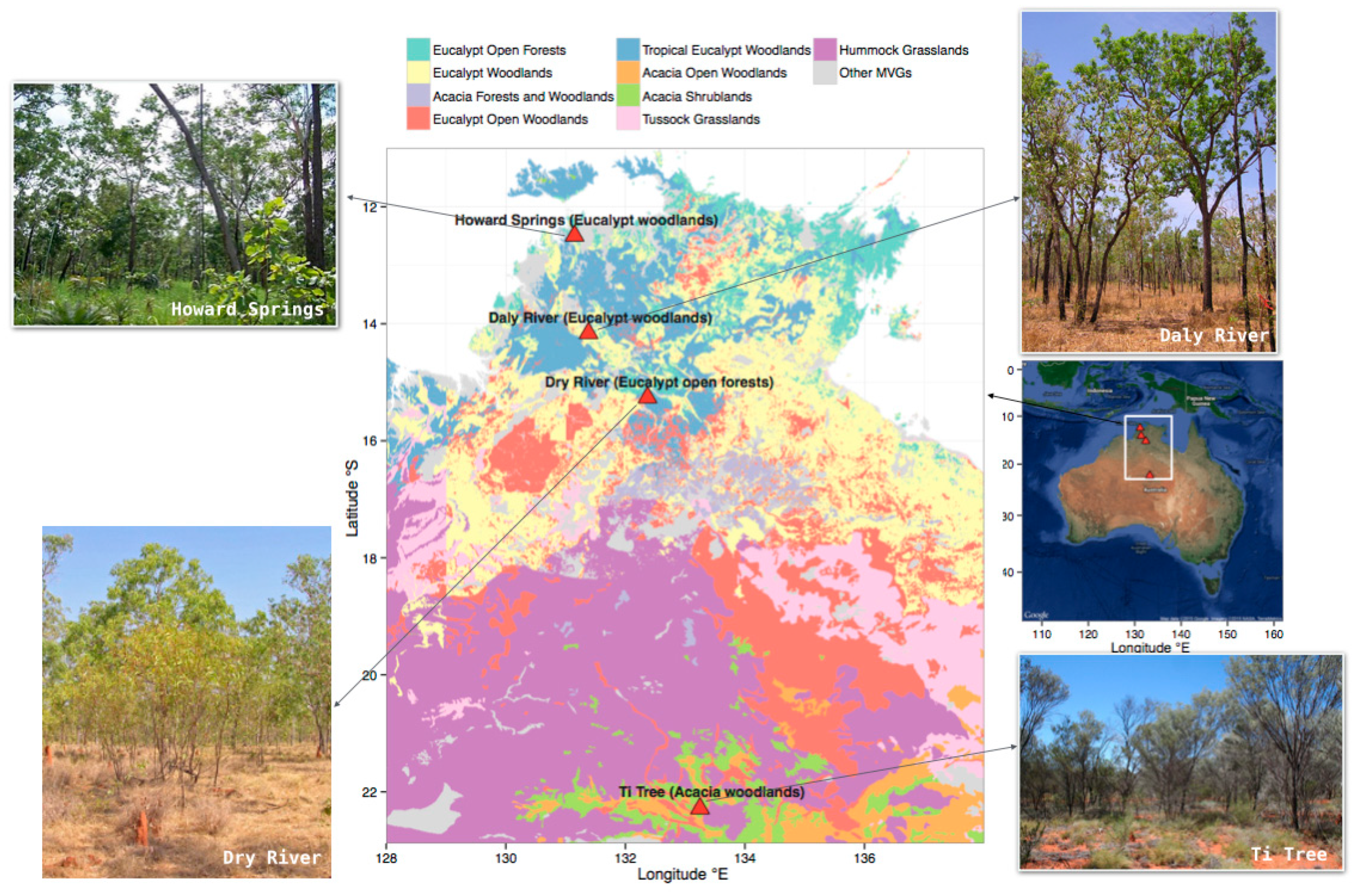
2.1. Study Area and Local Sites

The NATT is a sub-continental scale ecological rainfall gradient conceptualised in the mid-1990s, as part of the International Geosphere Biosphere Programme (IGBP) [24], to study global savannas (Figure 1). The vegetation of the entire transect follows a wet–dry savanna gradient that transitions from Eucalyptus-dominated forests and woodlands in the northern areas to Acacia-dominated woodlands and shrublands in the south. Mean annual precipitation decreases from over 1,700 mm in the northern mesic tropics to about 300 mm in the xeric southern region. Soils range from Kandosols (Palexeralfs in U.S. Taxonomy) and affiliated types at the northern humid end [25] to black cracking clay soils or sandy soils at the southern arid end [26]. Over the past few years, several satellite-/tower-based phenology studies have been performed at site- and regional-scales, over NATT [14,27,28].
Within this extensive transect study area, four well-characterised local sites were selected, representing different savanna vegetation structures/functional classes and rainfall regimes (Figure 1 and Table 1), to investigate the sun-angle effect on remote-sensing-derived phenology. These sites include three Eucalyptus woodland sites—Howard Springs, Daly River and Dry River [25], and an Acacia woodland site—Ti Tree [29,30].

2.2. BRDF Model

The surface reflectance can be described using a BRDF, which is a function of the solar zenith angle, view zenith angle, and both solar azimuth angle and view azimuth angle, with respect to a reference direction [31]. This anisotropy is strongly affected by solar illumination angle [18] as well as the canopy structural geometry and wavelength [18]. BRDF can be used to standardise surface reflectance observations with varying sun-view geometries to a common geometry [32].
In this study, a well-tested semi-empirical BRDF model, the RossThick-LiSparse Reciprocal model (hereafter, RTLS model), was implemented to simulate MODIS surface reflectances as acquired at varying solar zenith angles [33]. The theoretical basis of the semi-empirical BRDF model is that the land surface reflectance can be modelled as a sum of three kernels representing basic scattering types—isotropic scattering, radiative transfer-type volumetric scattering (similar to that from horizontally homogeneous leaf canopies), and geometric-optical surface scattering (similar to that from scenes containing three-dimensional objects that cast shadows and are mutually obscured from view at off-nadir angles) [31,34,35]. In this study, the three kernels of the BRDF model, which quantify intrinsic surface properties at any given site and within an eight-day period, were inverted from the MODIS observations (combined Terra and Aqua) [15].

2.3. Vegetation Indices

NDVI and EVI are widely used as proxies of canopy “greenness”, an integrative composite property of the green leaf area, canopy structure, and leaf chlorophyll content [36]. Both NDVI and EVI have been used for deriving vegetation phenological metrics at regional to global scales [5,37,38,39,40]. Vegetation Indices (VIs) are robust and seamless biophysical measures, computed identically across all pixels in time and space, regardless of the biome type, land cover condition and soil type [41]. EVI was used as an optimised version of NDVI that effectively reduces soil background influences and atmospheric noise variations [6]. The equations defining NDVI [42] and EVI are:
NDVI = ρ nir ρ red ρ nir + ρ red
EVI = 2.5 ρ nir ρ red ρ nir + 6 ρ red 7.5 ρ blue + 1
where ρnir, ρred and ρblue are reflectances of the near infrared (841–876 nm), red (620–670 nm), and blue (459–479 nm) bands of the MODIS sensor, respectively.

2.4. MOD09A1

We used 9 years (Jan 2010–Dec 2018) of 8-day 500 m Surface Reflectance products (MOD09A1, C006, tiles h30v10 and h30v11) [32] obtained through the online Data Pool at the NASA Land Processes Distributed Active Archive Centre (LP DAAC), the USGS/Earth Resources Observation and Science (EROS) Centre (https://lpdaac.usgs.gov/data_access). Solar zenith angle when the Terra overpassed (~10:30AM, termed as SZA-Terra for further reference) were extracted for each local site. The SZA-Terra was then used as an input variable to the RTLS BRDF model, together with the BRDF model parameters from MCD43A1, for simulating surface reflectance and calculating Vis, as when sun-angle was at the Terra overpassing time and when the view-angle was at nadir.

2.5. MCD43A1

We obtained 9 years (Jan 201–Dec 2018) of daily 500 m BRDF/Albedo Model Parameters product (MCD43A1 C006, tiles h30v10 and h30v11). The MCD43A1 product supplies the weighting parameters associated with the semi-empirical RTLS BRDF model that best describes the anisotropy of each pixel at any given 8-day period [15]. Combined data from the MODIS instruments onboard the Aqua and Terra satellites were used. A 3 × 3 MCD43A1 500 m pixel window (2.25 km2) was used to extract the time series of the BRDF parameters for each local site. Within the extracted time series, only good quality data with full BRDF model inversion were selected, according to the QA layer of MCD43A1.
A normalisation of the directional effect consists of putting the measurements in a standard observation geometry [32]. To focus on the effect of seasonal variations in SZA on surface reflectances and VIs, view zenith angle was normalised to zero (i.e., nadir view) and solar zenith angle was either varied at the Terra overpass time (SZA-Terra), local solar noon (this is the same configuration as the MCD43A4 NBAR product, termed as SZA-Local Solar Noon (SZA-LSN)), or was fixed at 0°, 15°, 35° and 45° (termed as SZA-0, SZA-15, SZA-30, SZA-45, respectively) to capture the widest possible range in SZA over the NATT study area.

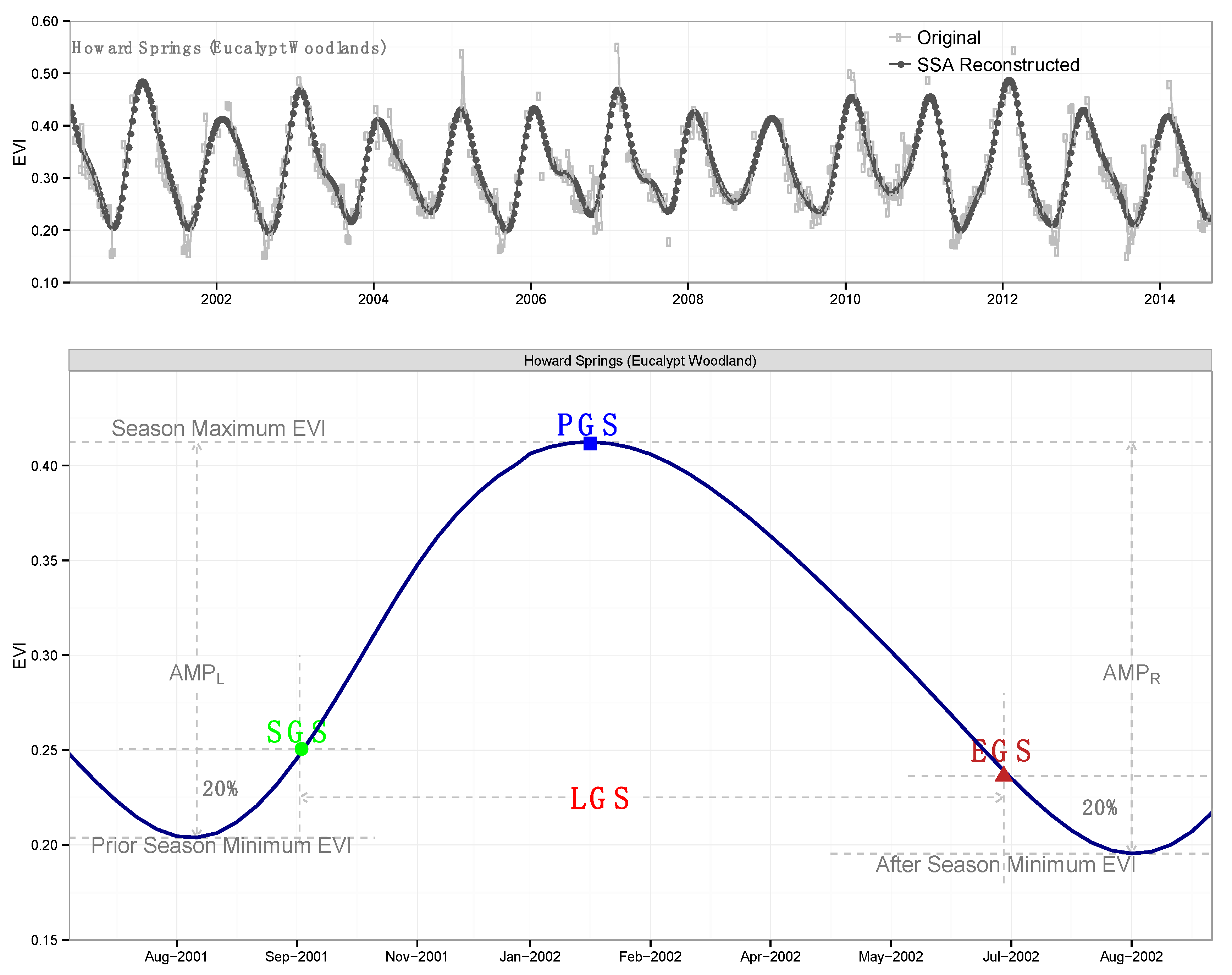
2.6. The Phenological Metrics Extraction Method

Figure 2 diagrams the method for extracting phenological metrics from the VI time series. Four phenological metrics, including the start of growing season (SGS), the peak of growing season (PGS), the end of growing season (EGS), and the length of growing season (LGS), were extracted from the time series of MODIS VI, using an algorithm based on Singular Spectrum Analysis (SSA-Pheno) [14]. The SSA-Pheno algorithm has been tested over Australia, across a wide-range of vegetation structural classes and rainfall regimes, and has demonstrated robustness and reliability in extracting phenological metrics from the noisy MODIS time series [14,43]. Technical description of the SSA-Pheno can be found in [14,43]. Here, we briefly introduce the concept of this algorithm and the main parameters used. The SSA (Singular Spectrum Analysis) is a data-adaptive method that has been found to be well-suited to the analysis of nonlinear dynamics in geophysical datasets. The fundamental concept of SSA is to embed a time series into a high-dimensional Euclidean space and identify the sub-space corresponding to the component of the interest from which a reconstructed time series is generated. SSA implementation requires two important parameters to be determined—the window length L and the selection of the leading components N. In testing our dataset, an optimised L of 46 composite periods (46 × 8 / 365 ≈ 1 year) was found to best capture the periodicity and reduce most of the high frequency random noise. We selected four leading components (N = 4) to reconstruct the VI time series, with the first component contributing information on the long-term trend and the remaining components contributing the periodicities of declining frequency, which are important for retrievals of the phenological metrics. Lastly, the SSA-reconstructed 8-day VI time series was interpolated to daily values using local polynomial regression, before being used to derive the phenological metrics.
In this study, SGS was defined as when VI reached the value equal to the minimum value prior to the growing season plus 20% of the seasonal amplitude, during the greenup phase. Similarly, EGS was defined as when VI reaches the value equal to the minimum value after greening season plus 20% of amplitude, during the browndown phase. LGS was calculated as the difference between EGS and SGS. Phenological metrics were only extracted when consecutive gaps within the time series of VIs were less than six for any given site/year.

2.7. Statistics

To evaluate the difference among phenological metrics derived from time series of VIs with different sun-angle configurations, the root mean squared error (RMSE) was calculated. The equation to calculate RMSE is:
RMSE = t = 1 n ( x 0 x ) 2 n
Data processing, statistical analysis, and visualisation were conducted in open source R scientific computation environment (Version 3.3.3) and associated packages contributed by the R user community (http://cran.r-project.org) [44].

3. Results

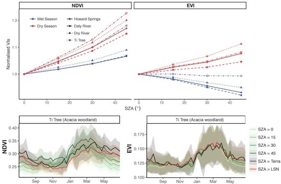
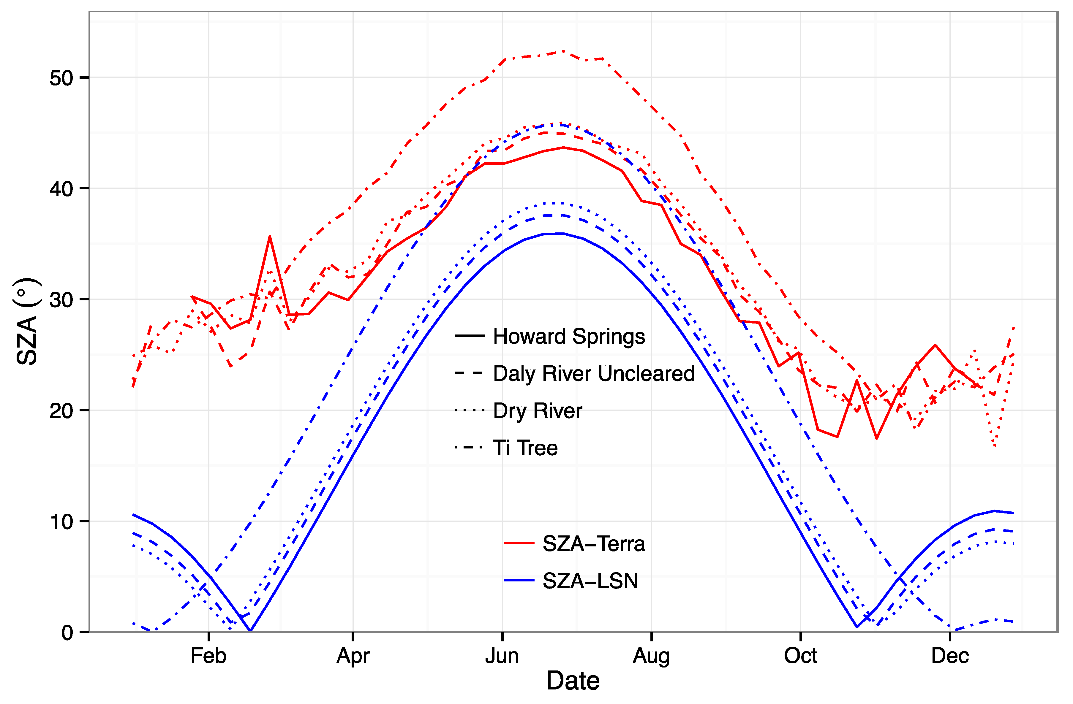
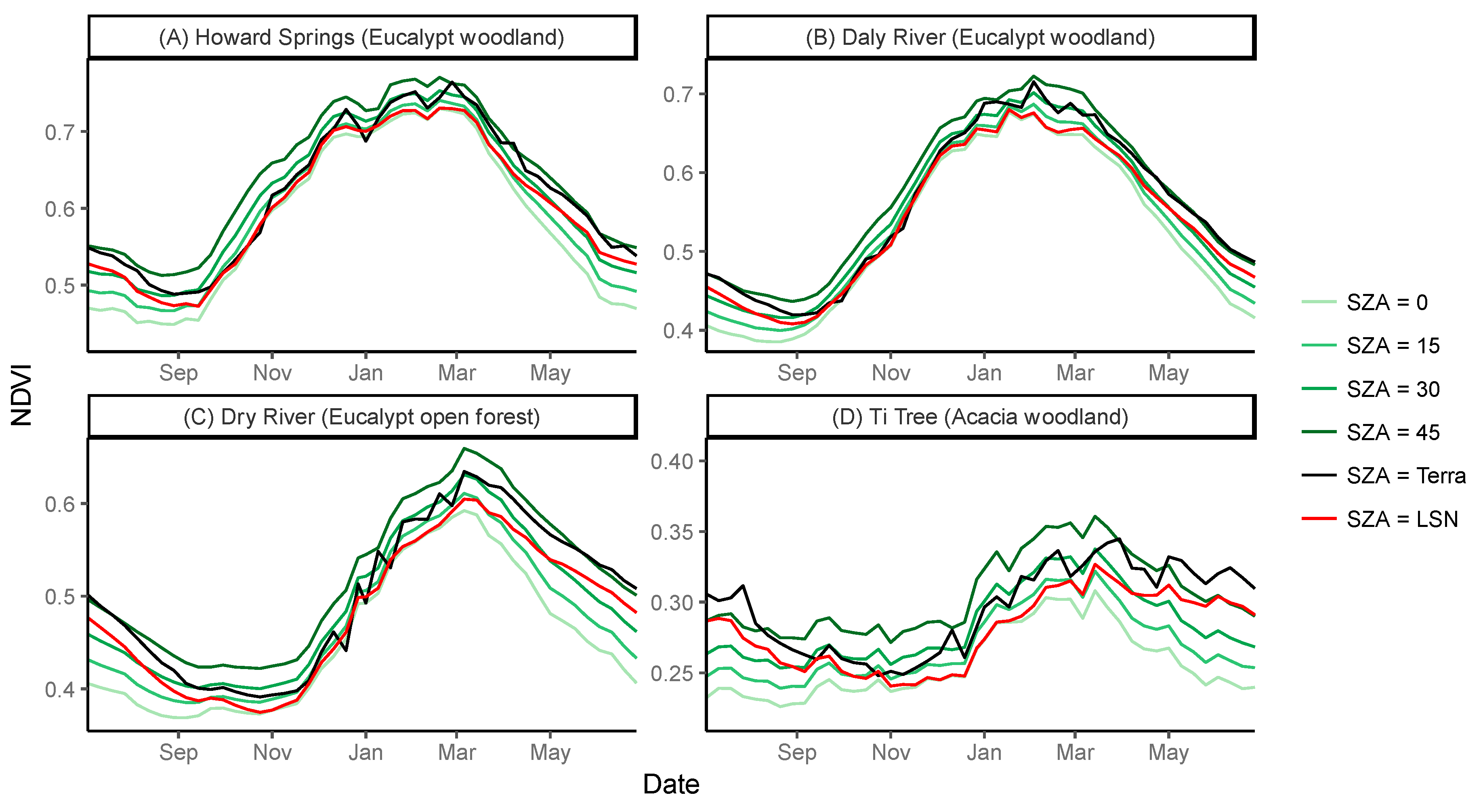
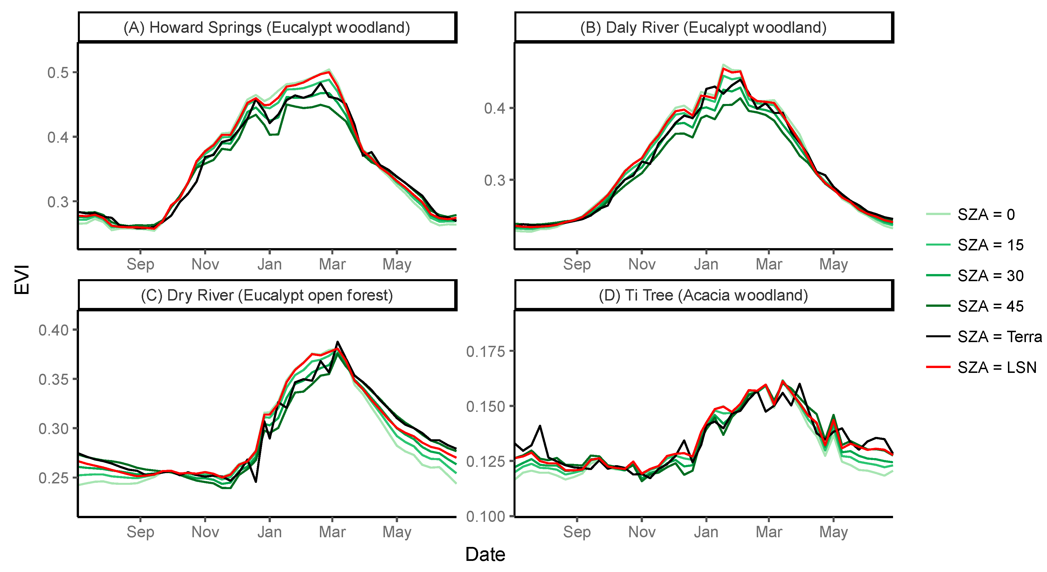
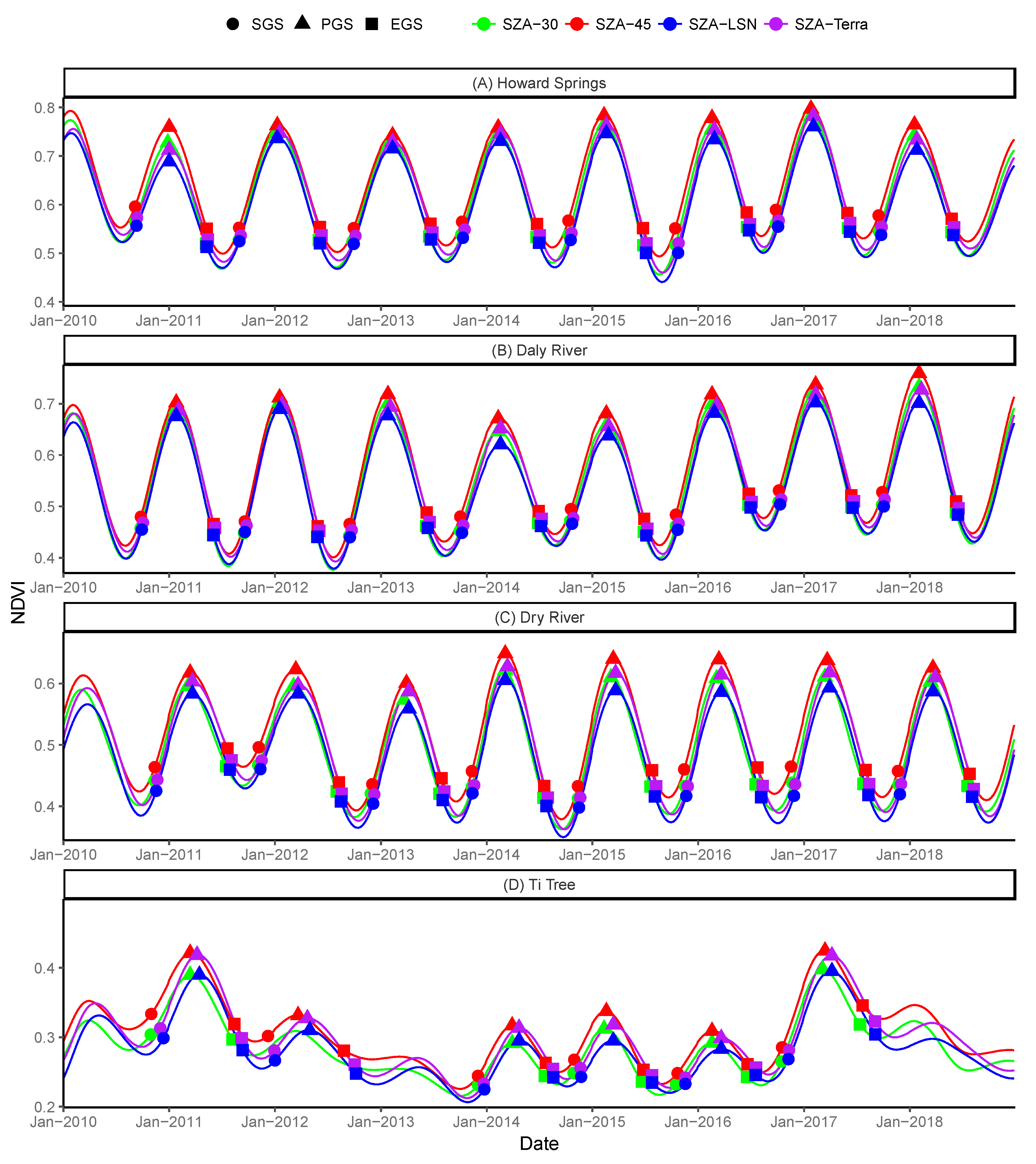
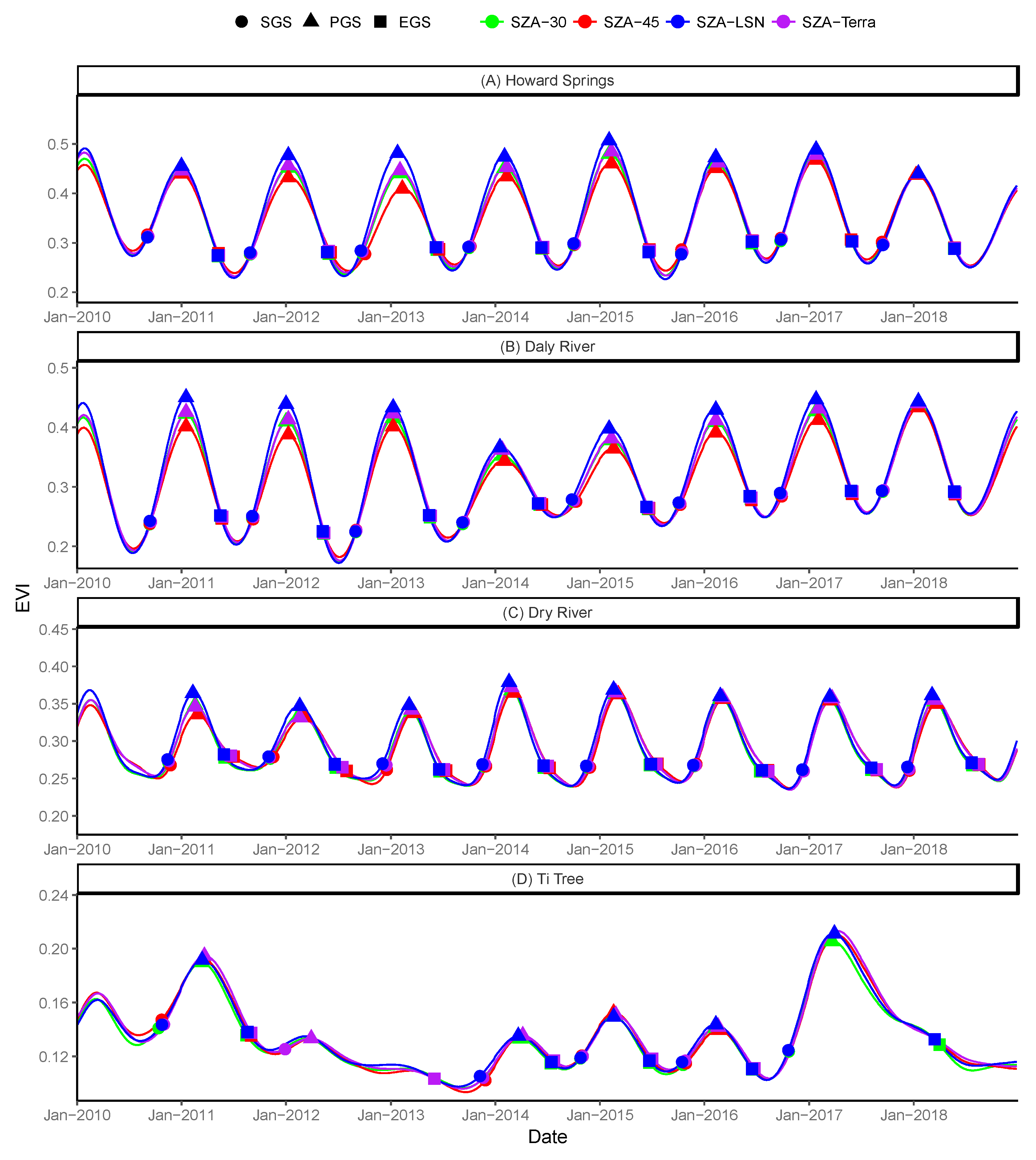
3.1. Seasonal Profiles of NDVI and EVI Normalised to Different Sun-Angles

Solar zenith angle (SZA) exhibited a seasonal cycle that also varied across sites (Figure 3). The range of seasonal variations in SZA increased with latitude, with the SZA-Terra ranging from about 17–44°, at Northern Howard Springs (12.5 °S) to about 18–52° at Southern Ti Tree (22.3 °S) (Figure 3). Seasonal dynamic ranges of SZA was enhanced by SZA-LSN, varying from about 0–36° at Howard Springs to about 0–46° at Ti Tree, all much larger than the observation range that the Terra satellite experiences (Figure 3).
Figure 4 and Figure 5 show the time series comparisons among mean seasonal profiles of NDVI or EVI, normalised to different SZAs at a nadir view. Differences in sun-angle configuration resulted in considerable differences in both the shape and magnitude of the phenological profiles, particularly during the browndown phase (peak to dry season) (Figure 4 and Figure 5). Differences among NDVIs were generally greater than the differences among EVIs, and the differences in the magnitude of sun-angle effect on time series of VIs were different across sites and vegetation types (Figure 4 and Figure 5). The sun-angle effect was larger at the Southern Dry River and Ti Tree sites where vegetation cover was sparser and seasonal variation in the sun-angle was larger as compared to the northern sites (Figure 4 and Figure 5).

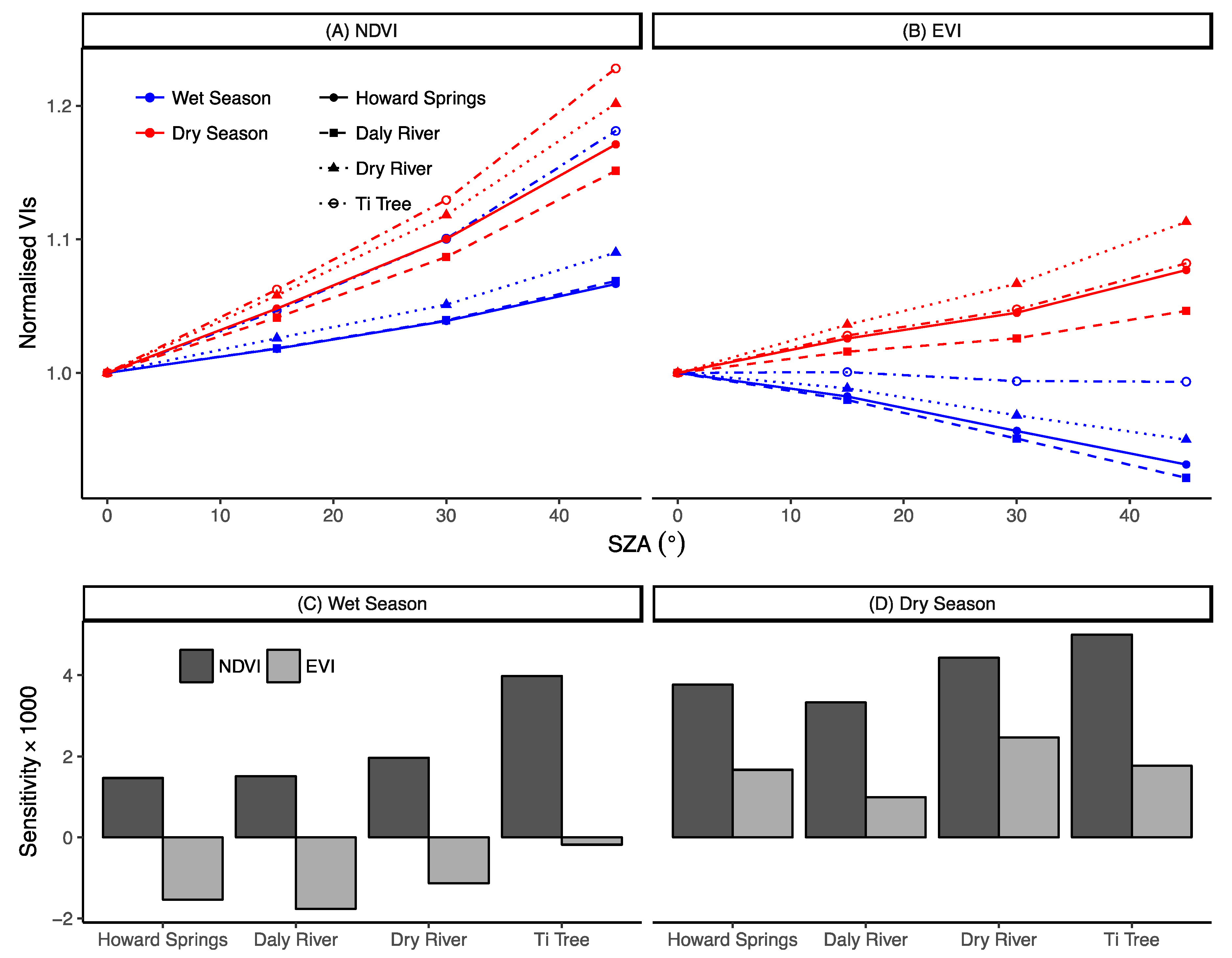
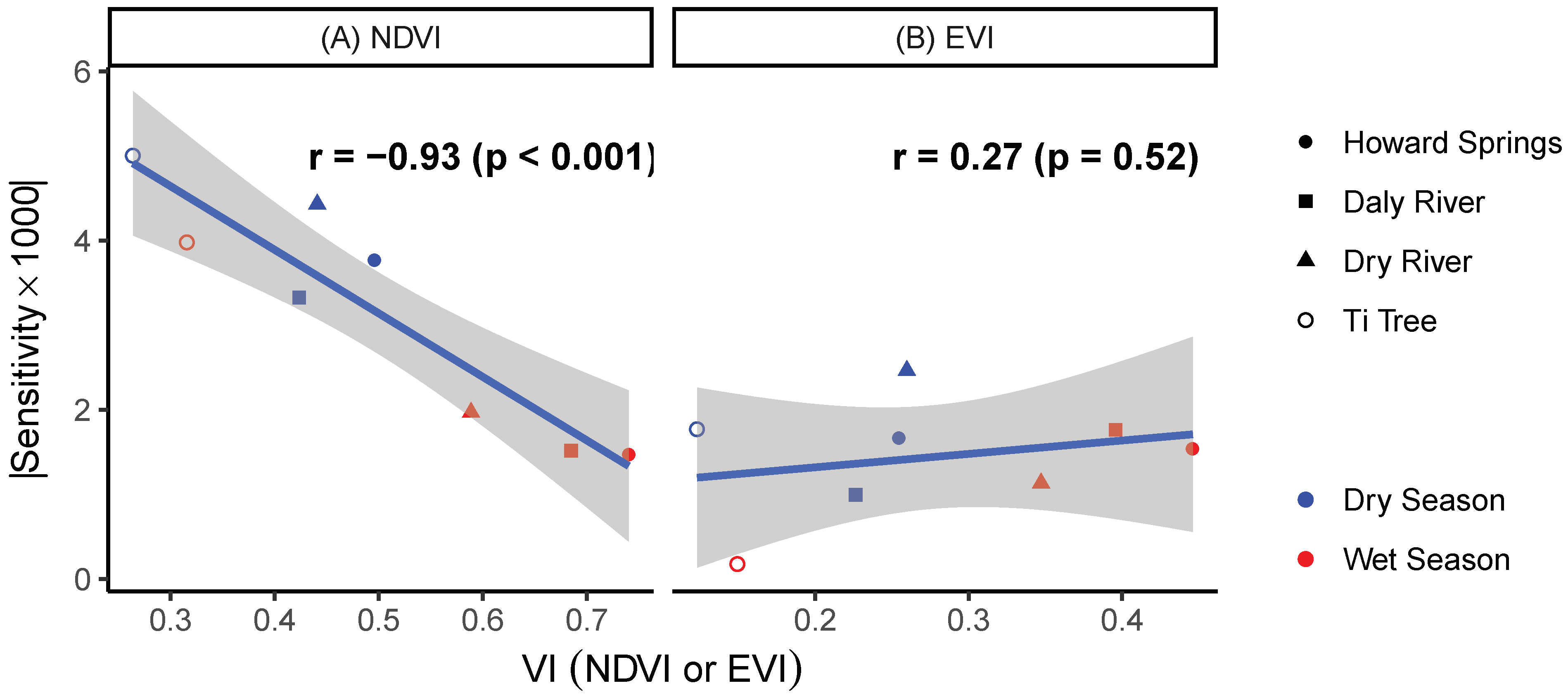
3.2. Variations in the Sensitivity of NDVI and EVI to Sun-Angle across Sites and Phenophases

To investigate the sensitivity of NDVI and EVI to sun-angle at any given date, VIs fixed at four sun-angles (all nadir view), VISZA-0, VISZA-15, VISZA-30 and VISZA-45, were plotted with respect to the sun-angle. Due to the seasonal variations in the quantity of greenness, the four VIs were normalised by VISZA-0 at any given site/date to focus on the slope (sensitivity) and percentage change relative to VISZA-0. There were considerable differences in the sensitivity of VIs to the sun-angle across sites, between the wet season (February) and the dry season (July), and between NDVI and EVI (Figure 6). First, sensitivity of VIs to sun-angle was generally larger during the dry season than during the wet season (except for EVI at the Daly River site) (Figure 6). Additionally, the dynamic range of the sensitivity of VIs to sun-angle was larger at Howard Springs, Daly River, and Dry River sites than at the Ti Tree site (Figure 6). Except for the wet season at Howard Springs and the Daly River sites, where the sensitivity of NDVI and EVI to SZA was similar, for the other sites, the sensitivity of NDVI to sun-angle was generally greater than the sensitivity of EVI during both the wet and dry seasons (Figure 6C,D).
Furthermore, only positive responses of NDVI to sun-angle variations were observed, while EVI exhibited both positive and negative responses (Figure 6C,D). During the dry season (with only evergreen trees present), EVI across all sites increased with increases in SZA, while during the wet season (with both trees and green grass present), EVI decreased with increasing SZA (Figure 6B). We further examined the relationship between VI sensitivity to SZA (in absolute values) as a measure of the overall sensitivity regardless of signs and vegetation cover (measured by NDVI or EVI), across sites and seasons (Figure 7). A strong negative correlation between NDVI sensitivity to SZA (in absolute value) and vegetation cover was observed (r = −0.93, p-value < 0.0001), while no significant correlation between EVI sensitivity to SZA (in absolute value) and EVI-level was observed (r = 0.27, p-value = 0.52) (Figure 7). On average, NDVI and EVI sensitivities to SZA were 0.0031 ± 0.0014 and 0.0003 ± 0.0007, per degree change in the SZA across site/season (Figure 7). It is also worth noting that only when vegetation cover approached very high levels (NDVI > 0.6), as during the wet season, did the NDVI sensitivity to SZA decline to low levels, comparable to those of EVI (Figure 7).

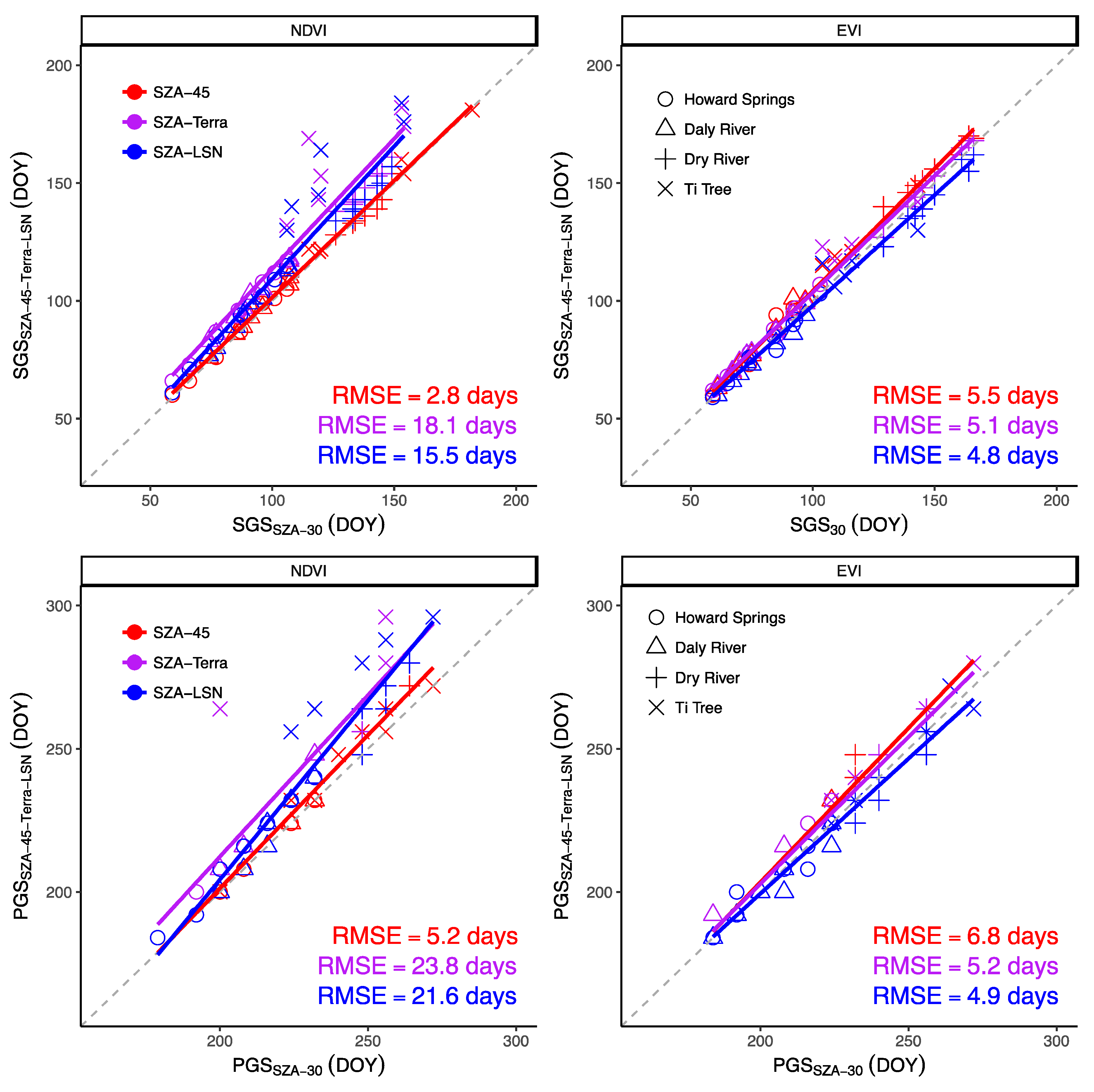
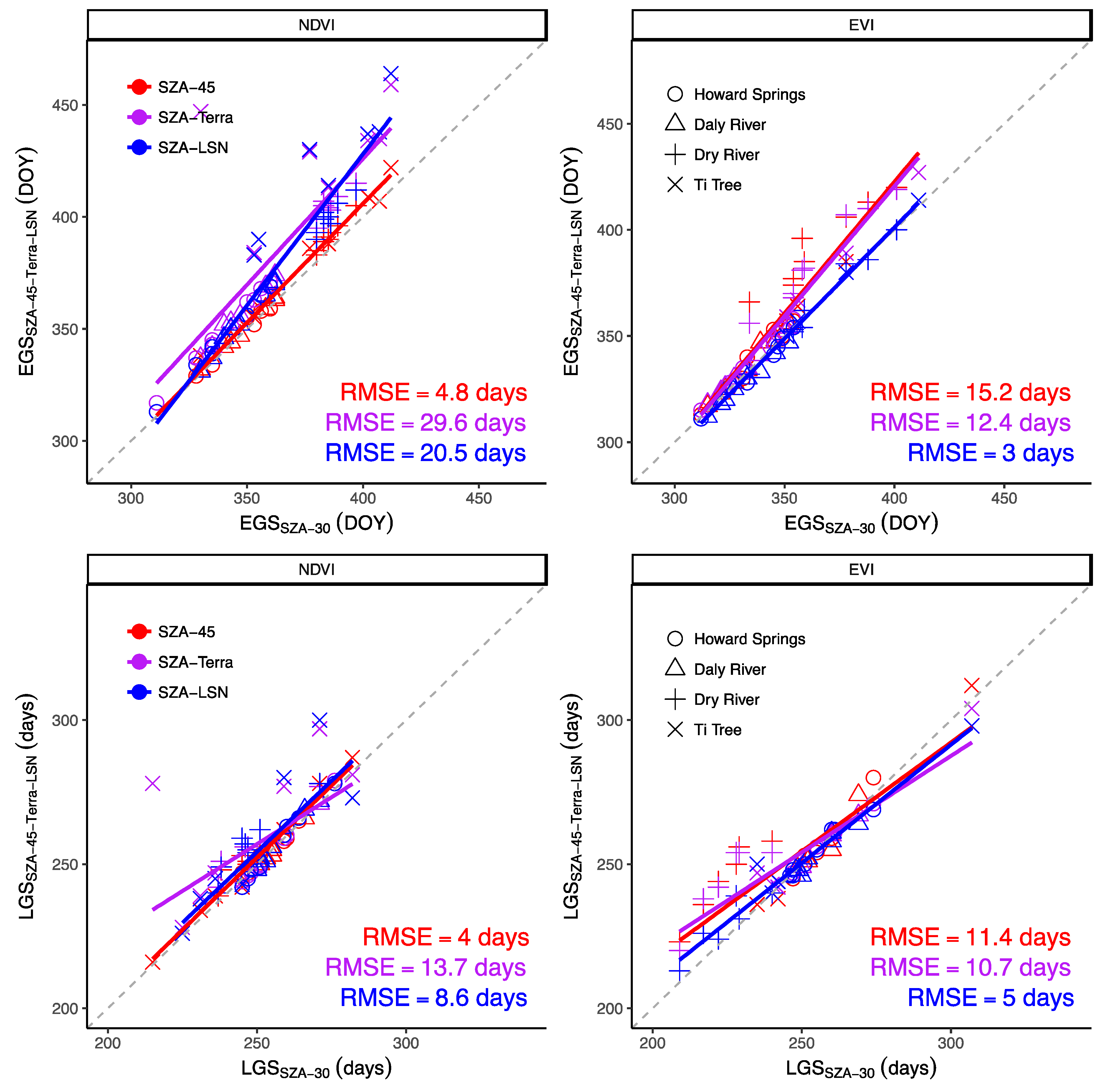
3.3. Impacts of the Sun-Angle on Phenological Metrics Derived from Time Series of VIs

Figure 8 and Figure 9 show the original and SSA-reconstructed time series of NDVI and EVI with different sun-angle configurations at the four NATT sites. Phenological transition dates extracted using SSA-Pheno algorithm were indicated on each plot. It can be seen that seasonal variations in sun-angle had a large impact on the derived phenological metrics and the impact was generally larger on the metrics derived from NDVI than the metrics derived from EVI (Figure 8 and Figure 9). Overall, the differences among metrics derived from the different VIs were relatively small at the Howard Springs and the Daly River sites (Figure 8A,B and Figure 9A,B) and increased at the Dry River site, and the differences were most pronounced at the Ti Tree site (Figure 8C,D and Figure 9C,D).
Figure 10 and Figure 11 show the cross-site comparisons among phenological metrics derived from VISZA-Terra, VISZA-LSN, VISZA-30 and VISZA-45, at the four NATT sites. Despite the use of a consistent phenological metrics retrieval algorithm, there were considerable differences among the metrics derived from Vis, with varying SZA (SZA-Terra and SZA-LSN) and metrics derived from VIs with fixed SZAs (Figure 10 and Figure 11). Varying sun-angle resulted in positive biases (i.e., delay) in NDVI-based phenological metrics, yet the impact of the varying sun-angle EVI-based metrics was more complex with both positive and negative biases observed across sites (Figure 10 and Figure 11). Phenological metrics derived from VISZA-Terra and VISZA-LSN exhibited discrepancies similar to those derived from VISZA-30 (Figure 10). Across the four sites, the sun-angle effects caused 15.5-day, 21.6-day and 20.5-day differences, respectively, in the start, peak, and end dates of growing season derived from NDVISZA-LSN, as compared to those derived from NDVISZA-30. In comparison, those differences, respectively, in the start, peak, and end dates of the growing season derived from EVISZA-LSN, as compared to EVISZA-30 were considerably smaller and were only less than 5 days.

4. Discussion

One of the objectives of this study was to evaluate the sensitivities of two commonly used vegetation indices—NDVI and EVI—to seasonal variations in the sun-angle. Considerable variations in the sensitivity of NDVI and EVI were found across the different phenological stages. At any given site/date, NDVI increased with increasing sun-angle (Figure 6). However, EVI appears to be largely immune to sun-angle effects (Figure 7). At any given site/date, EVI can both increase or decrease with increases in sun-angle, depending on the phenological stage (wet or dry seasons) (Figure 6). Our findings here over tropical savannas were in line with the previous findings by Middleton [18] in a tall grass prairie, which also found that at intermediate biomass sites (0.5 < LAI < 2.0), NDVI increased with solar zenith angle. Similar monotonic increases in NDVI with solar zenith angle have also been reported elsewhere, for alfalfa [21,45] and the Amazon tropical forest [46].
Our finding that NDVI was more sensitive to SZA variations at the southern xeric sites with sparse vegetation cover than at the northern humid dense vegetated woodland was consistent with previous studies which showed the trend of decrease in sensitivity of NDVI to SZA, as leaf area increased [47]. This assumption was further corroborated by the analysis between NDVI sensitivity to SZA with regard to vegetation cover, with two interesting observations—(1) a strong negative correlation and (2) an NDVI sensitivity decline to the same low levels as the EVI, when vegetation cover was high (Figure 7). This could be explained by the fact that under dense vegetation canopies, the influence of soil-induced effect was minimal [47]. Additionally, the saturation of NDVI in high biomass areas might also explain the declined sensitivity of NDVI to SZA variations [47,48]. Our findings of the EVI being consistently less sensitive than NDVI to SZA variations across most site and seasons (Figure 6) adds more vegetation types to [9], which also found that EVI was more resistant to variations in viewing and illumination geometry, when compared to NDVI in tropical forests.
The positive and negative responses of EVI to sun-angle variations were intriguing, which suggested there might be potential factors, such as vegetation structure and phenological stages that dictated the sign of the EVI response to the sun-angle. For instance, it has been observed that canopy reflectance increased, decreased, or remained invariant with changing solar angles, depending on the reflectance properties of the underlying soil [17]. Our finding of varying response of VIs to sun-angles, across phenophases, might also reflect the relative role of vegetation cover and soil background in determining the sun-angle effect on VIs, especially for NDVI (Figure 7).
The response patterns of vegetation indices to SZA are different across phenological seasons and across different vegetation structural classes. The different responses of VIs to sun-angles, precluded the use of a simple correction method to remove the sun-angle effect, which implied that knowledge of site-specific canopy and soil attributes at the time of observation are essential for a full-correction of the sun-angle effect on surface reflectances [17,18]. In addition, a standard SZA has to be predefined for real-time normalisation of the sun-angle to constant illumination conditions, across space and time.
Our results also showed that both the shape and magnitude of the seasonal profiles of NDVI and EVI were significantly altered by sun-angle variations, resulting in considerable differences among phenological metrics derived from VIs with variable SZA configurations. Vegetation indices calculated using MCD43A4 nadir-adjusted (NBAR) surface reflectances have been widely used for deriving phenological metrics at the regional to global scales [5,49]. The NBAR product provides reflectance data adjusted to the nadir view, but SZA remains variable across seasons (local solar noon) [15].
In addition, because different plant functional types (or species) can have unique phenologies and these would affect how seasonal VI profile is coupled with the seasonal sun-angle variation, leading to a stronger or a weaker sun-angle dependency of the retrieved phenological metrics. Future studies might consider not only vegetation structural classes but also functional classes to better understand and disentangle the relative influence of these two on the interaction of seasonal sun-angle and vegetation phenology.
On a global monitoring scale, the sun-angle effect could result in uncertainties in the estimation of several important ecological parameters, such as carbon uptake period, grass curing, and crop/forage productions, particularly at high-latitudes where seasonal variations in solar zenith angle are larger than tropic and sub-tropic regions. As such, the findings from our study should have important ecological implications on studies related to terrestrial carbon cycle, food security and fire management. For example, a previous study noticed that the length of growing season tended to be overestimated in the Southern Hemisphere by pathfinder NDVI, if the BRDF effect was not corrected [22]. To obtain a realistic representation of ground vegetation dynamics using satellite observations, it was, therefore, of great importance that both the sun-angle and view-angle effects on surface reflectances were properly corrected before extracting the phenological metrics from these observations.
However, it must be admitted that having a global near-real-time correction of the sun-angle effect is not as intuitive as having a correction of view-angle effect. This is due to two major reasons. First, the restriction of nadir surface reflectances measurements to a fixed SZA is still not practical for the current polar-orbiting satellites. In this sense, the increasing availability of data streams from new generation geostationary satellites with a refined spatial resolution, has the potential to be used to normalise SZA, as within any given day, observations can be selected according to the hour of the (hence, SZA). Second, an arbitrary sun-angle has to be predefined and one has to assume such an angle is applicable over the entire globe and across seasons. It is obvious that such an assumption would result in half of the planet at any given date being modelled to an unrealistic sun angle that never occurs in reality, and thus, cannot be validated through comparison with ground measurements. Nevertheless, the correction of the sun-angle effect would still be largely possible and valuable for a regional vegetation and crop monitoring scheme.
Previous studies in northern temperate regions generally defined 45° as a standard SZA [18,50]. However, 45° would be too large for tropical areas, as most observations taken by Terra and Aqua were in a situation when SZA was below 45° in the NATT study area (Figure 3), thus, using 45° as standard SZA would result in consistent over-extrapolation of the BRDF model. As a result, a trade-off has to be nonetheless made for normalising SZA across space or time, depending on the research emphasis (e.g., trend in phenology across time at any given location or spatial patterns in phenology over a regional scale).
The selection of a standard SZA brings to mind the question asked by Middleton in 1992: “Which solar zenith angle is best for acquiring surface reflectance measurements in order to monitor vegetation dynamics and to estimate canopy structural and functional variables?” [18]. During the past decades, the launches of Terra, Aqua and NPP satellites and the subsequent release of publicly-available MODIS/VIIRS products, brought about a rich era in the applications of satellite observations in agriculture, ecology, environment and global change studies. However, global products are still lacking for surface reflectances and vegetation indices that have been fully-corrected for the BRDF effect.
In summary, future studies are urgently needed to improve our understanding of the sun-angle effect on vegetation indices and phenological metrics, and to determine whether an optimal method exists for the correction of sun-angle effects at a global scale. This would not only facilitate more meaningful comparisons of vegetation greenness and productivity at a global scale for climate continuity analysis, but would also improve the monitoring of real biological signals that are free from artefacts caused by directional effects.

5. Conclusions

Satellite-based studies of vegetation phenology generally rely on time series of vegetation indices, either without correction of changing viewing and illumination geometries (e.g., MOD09 or MOD13), or only with partial correction of the view-angle effect (e.g., MCD43 NBAR). In this study, the sun-angle effect on NDVI and EVI was examined through a complete simulation of surface reflectances, with multiple sun-angle configurations. The influences of seasonal sun-angle variations on several phenological transition dates were further assessed.
Our results showed that NDVI and EVI are both sensitive to variations in SZA, and NDVI is much more sensitive to SZA than EVI. The sun-angle effects result in considerable differences in both the shape and magnitude of the phenological profiles. Responses of NDVI and EVI to SZA variations are not only dependent on vegetation structural classes, but also exhibit dependencies on phenophases with contrasting responses of VIs to sun-angle variations, across different stages of the growing seasons. Phenological metrics derived from NDVI without the correction of sun-angle effect are biased, as compared to those derived from VIs with a standard sun-view geometry, and such bias is possibly absent for EVI, probably due to an overall smaller sensitivity of EVI to SZA. Furthermore, phenological metrics derived from VIs fixed at different, constant sun-angles, also show discrepancies, suggesting that the selection of a constant SZA for normalisation of the sun-angle effects is relevant for deriving consistent and comparable phenological metrics, across space and time.
One of the priorities of terrestrial remote sensing is to identify the signals of seasonal and inter-annual dynamics of vegetation, in response to climate change and human activities, and distinguish such signals from noise and artefacts caused by external factors. As restrictive nadir VI observations at fixed sun-angles are not currently feasible from sensor measurements onboard the current satellites, the BRDF-model should be used for normalising satellite observations to a standard sun-view geometry, before deriving phenological metrics from the time series of satellite observations.

Author Contributions

Conceptualization, X.M. and A.H.; Formal analysis, X.M. and N.N.T.; Funding acquisition, A.H.; Investigation, X.M. and N.N.T.; Methodology, X.M. and N.N.T.; Supervision, A.H.; Visualization, X.M.; Writing—original draft, X.M., A.H. and N.N.T.; Writing—review and editing, X.M.

Funding

This research was funded by the AusCover Facility of the Australian Terrestrial Ecosystem Research Network (TERN) (http://www.tern.org.au).

Acknowledgments

This work was finished within the framework of the TERN—AusCover Land Surface Phenology product (http://www.auscover.org.au/purl/modis-phenology-uts) as developed by the Ecosystem Dynamics, Health and Resilience Research Group of the University of Technology Sydney (CI Huete).

Conflicts of Interest

The authors declare no conflict of interest.

References

  1. White, M.; Thornton, P. A continental phenology model for monitoring vegetation responses to interannual climatic variability. Glob. Biogeochem. Cycles 1997, 11, 217–234. [Google Scholar] [CrossRef]
  2. Running, S.; Hunt, E. Generalization of a forest ecosystem process model for other biomes, BIOME-BGC, and an application for global-scale models. In Scaling Physiological Processes from Leaf to Globe; Ehleringer, J., Field, C., Eds.; Academic Press: San Diego, CA, USA, 1993; pp. 141–158. [Google Scholar]
  3. Piao, S.; Fang, J.; Zhou, L.; Ciais, P.; Zhu, B. Variations in satellite-derived phenology in China’s temperate vegetation. Glob. Chang. Biol. 2006, 12, 672–685. [Google Scholar] [CrossRef]
  4. Richardson, A.; Anderson, R.; Altaf, A.; Barr, A.; Bohrer, B.; Chen, G.; Chen, J.M.; Ciais, P.; Davis, K.J.; Desai, A.R.; et al. Terrestrial biosphere models need better representation of vegetation phenology: Results from the North American Carbon Program Site Synthesis. Glob. Chang. Biol. 2012, 18, 566–584. [Google Scholar] [CrossRef]
  5. Zhang, X.; Friedl, M.; Schaaf, C.; Strahler, A.; Hodges, H.; Gao, F.; Reed, B.; Huete, A. Monitoring vegetation phenology using MODIS. Remote Sens. Environ. 2003, 84, 471–475. [Google Scholar] [CrossRef]
  6. Huete, A.; Didan, K.; Miura, T.; Rodriguez, E.; Gao, X.; Ferreira, L. Overview of the radiometric and biophysical performance of the MODIS vegetation indices. Remote Sens. Environ. 2002, 83, 195–213. [Google Scholar] [CrossRef]
  7. Pinter, P.; Zipoli, G.; Maracchi, G.; Reginato, R. Influence of topography and sensor view angles on NIR red ratio and greenness vegetation indices of wheat. Int. J. Remote Sens. 1987, 8, 953–957. [Google Scholar] [CrossRef]
  8. Moura, Y.; Galvão, L.; Santos dos, J.; Roberts, D.; Breuning, F. Use of MISR/Terra data to study intra- and inter-annual EVI variations in the dry season of tropical forest. Remote Sens. Environ. 2012, 127, 260–270. [Google Scholar] [CrossRef]
  9. Bhandari, S.; Phinn, S.; Gill, T. Assessing viewing and illumination geometry effects on the MODIS vegetation index (MOD13Q1) time series: Implication for monitoring phenology and disturbances in forest communities in Queensland, Australia. Int. J. Remote Sens. 2011, 32, 7513–7538. [Google Scholar] [CrossRef]
  10. Sims, D.; Rahman, A.; Vermote, E.; Jiang, Z. Seasonal and inter-annual variation in view angle effects on MODIS vegetation indices at three forest sites. Remote Sens. Environ. 2011, 115, 3112–3120. [Google Scholar] [CrossRef]
  11. Maignan, F.; Breon, F.; Lacaze, R. Bidirectional reflectance of Earth targets: Evaluation of analytical models using a large set of spaceborne measurements with emphasis on the Hot Spot. Remote Sens. Environ. 2004, 90, 210–220. [Google Scholar] [CrossRef]
  12. Reed, B.; Brown, J.; VanderZee, D.; Loveland, T.; Merchant, J.; Ohlen, D. Measuring phenological variability from satellite imagery. J. Veg. Sci. 1994, 5, 703–714. [Google Scholar] [CrossRef]
  13. Beck, P.; Atzberger, C.; Høgda, K.; Johansen, B.; Skidmore, A. Improved monitoring of vegetation dynamics at very high latitudes: A new method using MODIS NDVI. Remote Sens. Environ. 2006, 100, 321–334. [Google Scholar] [CrossRef]
  14. Ma, X.; Huete, A.; Yu, Q.; Restrepo-Coupe, N.; Davies, K.; Broich, M.; Ratana, P.; Beringer, J.; Hutley, L.B.; Cleverly, J.; et al. Spatial patterns and temporal dynamics in savanna vegetation phenology across the North Australian Tropical Transect. Remote Sens. Environ. 2013, 139, 97–115. [Google Scholar] [CrossRef]
  15. Schaaf, C.; Gao, F.; Strahler, A.; Lucht, W.; Li, X.; Tsang, T.; Strugnell, N.C.; Zhang, X.; Jin, Y.; Muller, J.; et al. First operational BRDF, albedo nadir reflectance products from MODIS. Remote Sens. Environ. 2002, 83, 135–148. [Google Scholar] [CrossRef] [Green Version]
  16. Wang, Z.; Schaaf, C.; Sun, Q.; Shuai, Y.; Román, M. Capturing rapid land surface dynamics within collection V006 MODIS BRDF/NBAR/Albedo (MCD43) products. Remote Sens. Environ. 2018, 207, 50–64. [Google Scholar] [CrossRef]
  17. Huete, A. Soil and sun angle interactions on partial canopy spectra. Int. J. Remote Sens. 1987, 8, 1307–1317. [Google Scholar] [CrossRef]
  18. Middleton, E. Quantifying reflectance anisotropy of photosynthetically active radiation in grasslands. J. Geophys. Res. Biogeosci. 1992, 97, 18935–18946. [Google Scholar] [CrossRef]
  19. Morton, D.; Nagol, J.; Carabajal, C.; Rosette, J.; Palace, M.; Cook, B.; Vermote, E.F.; Harding, D.J.; North, P.R.J. Amazon forests maintain consistent canopy structure and greenness during the dry season. Nature 2014, 506, 221–224. [Google Scholar] [CrossRef]
  20. Gutman, G. On the use of long-term global data of land reflectances and vegetation indices derived from the advanced very high resolution radiometer. J. Geophys. Res. Biogeosci. 1999, 104, 6241–6255. [Google Scholar] [CrossRef]
  21. Pinter, P. Solar angle independence in the relationship between absorbed PAR and remotely sensed data for alfalfa. Remote Sens. Environ. 1993, 46, 19–25. [Google Scholar] [CrossRef]
  22. Los, S.; North, P.; Grey, W.; Barnsley, M. A method to convert AVHRR Normalized Difference Vegetation Index time series to a standard viewing and illumination geometry. Remote Sens. Environ. 2005, 99, 400–411. [Google Scholar] [CrossRef]
  23. Nagol, J.; Vermote, E.; Prince, S. Quantification of impact of orbital drift on inter-annual trends in AVHRR NDVI data. Remote Sens. 2014, 6, 6680–6687. [Google Scholar] [CrossRef]
  24. Koch, G.; Vitousek, P.; Steffen, W.; Walker, B. Terrestrial transects for global change research. Vegetatio 1995, 121, 53–65. [Google Scholar] [CrossRef]
  25. Beringer, J.; Hutley, L.; Hacker, J.; Neininger, B.; Paw, U. Patterns and processes of carbon, water and energy cycles across northern Australian landscapes: From point to region. Agric. For. Meteorol. 2011, 151, 1409–1416. [Google Scholar] [CrossRef]
  26. Walker, B.; Steffen, W.; Canadell, J.; Ingram, J. The Terrestrial Biosphere and Global Change: Implications for Natural and Managed Ecosystems Synthesis Volume; IGBP Book Series No. 4; Cambridge University Press: Cambridge, UK, 1999. [Google Scholar]
  27. Moore, C.; Beringer, J.; Evans, B.; Hutley, L.; McHugh, I.; Tapper, N. The contribution of trees and grasses to productivity of an Australian tropical savannas. Biogeosciences 2016, 13, 2387–2403. [Google Scholar] [CrossRef]
  28. Wang, C.; Beringer, J.; Hutley, L.; Cleverly, J.; Li, J.; Liu, Q.; Sun, Y. Phenology dynamics of dryland ecosystems along North Australian Tropical Transect revealed by satellite solar-induced chlorophyll fluorescence. Geophys. Res. Lett. 2019. [Google Scholar] [CrossRef]
  29. Eamus, D.; Cleverly, J.; Boulain, N.; Grant, N.; Faux, R.; Villalobos-Vega, R. Carbon and water fluxes in an arid-zone Acacia savanna woodland: An analyses of seasonal patterns and responses to rainfall events. Agric. For. Meteorol. 2013, 182–183, 225–238. [Google Scholar] [CrossRef]
  30. Cleverly, J.; Boulain, N.; Villalobos-Vega, R.; Grant, N.; Faux, R.; Wood, C.; Cook, P.G.; Yu, Q.; Leigh, A.; Eamus, D. Dynamics of component carbon fluxes in a semi-arid Acacia woodland, central Australia. J. Geophys. Res. Biogeosci. 2013, 118, 1168–1185. [Google Scholar] [CrossRef]
  31. Roujean, J.; Leroy, M.; Deschamps, P. A bidirectional reflectance model of the Earth’s surface for the correction of remote sensing data. J. Geophys. Res. Biogeosci. 1992, 97, 20455–20468. [Google Scholar] [CrossRef]
  32. Vermote, E.; Justice, C.; Breon, F. Towards a generalized approach for correction of the BRDF effect in MODIS directional reflectance. IEEE Trans. Geosci. Remote Sens. 2009, 47, 898–908. [Google Scholar] [CrossRef]
  33. Lucht, W.; Schaaf, C.; Strahler, A. An algorithm for the retrieval of albedo from space using semiempirical BRDF models. IEEE Trans. Geosci. Remote Sens. 2000, 38, 977–998. [Google Scholar] [CrossRef] [Green Version]
  34. Strahler, A.; Muller, J.; Lucht, W.; Schaaf, C. MODIS BRDF/albedo Product: Algorithm Theoretical Basis Document Version 5.0. Available online: https://modis.gsfc.nasa.gov/data/atbd/atbd_mod09.pdf (accessed on 10 June 2019).
  35. Li, X.; Strahler, A. geometric-optical bidirectional reflectance modeling of the discrete crown vegetation canopy. IEEE Trans. Geosci. Remote Sens. 1992, 30, 276–292. [Google Scholar] [CrossRef]
  36. Myneni, R.; Hall, F.; Sellers, P.; Marshak, A. The interpretation of spectral vegetation indices. IEEE Trans. Geosci. Remote Sens. 1995, 33, 481–486. [Google Scholar] [CrossRef]
  37. De Beurs, K.; Henebry, G. Land surface phenology and temperature variation in the International Geosphere-Biosphere Program high-latitude transects. Glob. Chang. Biol. 2005, 11, 779–790. [Google Scholar] [CrossRef]
  38. Jeganathan, C.; Dash, J.; Atkinson, P. Remote sensed trends in the phenology of northern high latitude terrestrial vegetation, controlling for land cover change and vegetation type. Remote Sens. Environ. 2014, 143, 154–170. [Google Scholar] [CrossRef]
  39. Broich, M.; Huete, A.; Paget, M.; Ma, X.; Tulbure, M.; Restrepo-Coupe, N.; Evans, B.; Beringer, J.; Devadas, R.; Davies, K.; et al. A spatially explicit land surface phenology data product for science, monitoring and natural resources management applications. Environ. Model. Softw. 2015, 64, 191–204. [Google Scholar] [CrossRef]
  40. Zhang, X.; Liu, L.; Jayavelu, S.; Wang, J.; Moon, M.; Moon, M.; Henebry, G.M.; Friedl, M.A.; Schaaf, C.B. Generation and evaluation of the VIIRS land surface phenology product. Remote Sens. Environ. 2018, 216, 212–229. [Google Scholar] [CrossRef]
  41. Huete, A.; Glenn, E. Remote sensing of ecosystem structure and function. In Advances in Environmental Remote Sensing: Sensors, Algorithms, and Applications; Taylor and Francis Gropu: Boca Raton, FL, USA, 2011; pp. 291–320. [Google Scholar]
  42. Rouse, J.; Haas, R.; Schell, J.; Deering, D. Monitoring vegetation systems in the Great Plains with ERTS. In Third Earth Resources Technology Satellite-1 Symposium. Technical Presentations, Section A, Vol. I; Freden, S.C., Mercanti, E.P., Becker, M., Eds.; NASA SP-351; National Aeronautics and Space Administration: Washington, DC, USA, 1973; pp. 309–317. [Google Scholar]
  43. Ma, X.; Huete, A.; Moran, M.; Ponce-Campos, G.; Eamus, D. Abrupt shifts in phenology and vegetation productivity under climate extremes. J. Geophys. Res. Biogeosci. 2015, 120, 2036–2052. [Google Scholar] [CrossRef]
  44. R Core Team. R: A Language and Environment for Statistical Computing; R Foundation for Statistical Computing: Vienna, Austria, 2017. [Google Scholar]
  45. Walter-Shea, E.; Privette, J.; Cornell, D. Relations between directional spectral vegetation indices and leaf area and absorbed radiation in alfalfa. Remote Sens. Environ. 1997, 61, 162–177. [Google Scholar] [CrossRef]
  46. Galvão, L.; Ponzoni, F.; Epiphanio, J.; Rudorff, B.; Formaggio, A. Sun and view angle effects on NDVI determination of land cover types in the Brazilian Amazon region with hyperspectral data. Int. J. Remote Sens. 2004, 25, 1861–1879. [Google Scholar] [CrossRef]
  47. Huete, A.; Liu, H.; van Leeuwen, W. The use of vegetation indices in forested regions: Issues of linearity and saturation. In Proceedings of the 1997 IEEE International Geoscience and Remote Sensing Symposium, Singapore, 3–8 August 1997; pp. 1966–1968. [Google Scholar] [CrossRef]
  48. Liu, G.; Liu, H.; Yin, Y. Global patterns of NDVI-indicated vegetation extremes and their sensitivity to climate extremes. Environ. Res. Lett. 2013, 8, 025009. [Google Scholar] [CrossRef] [Green Version]
  49. De Beurs, K.; Wright, C.; Henebry, G. Dual scale trend analysis for evaluating climatic and anthropogenic effects on the vegetated land surface in Russia and Kazakhstan. Environ. Res. Lett. 2009, 4, 045012. [Google Scholar] [CrossRef]
  50. Bréon, F.; Vermote, E. Correction of MODIS surface reflectance time series for BRDF effects. Remote Sens. Environ. 2012, 125, 1–9. [Google Scholar] [CrossRef]
Figure 1. Spatial extent of the North Australian Tropical Transect (NATT) study area. The red triangles indicate the locations of the four local sites. Background is the map of the Australian Major Vegetation Groups (MVGs, V4.1), provided by the Australian National Vegetation Information System. Central-right panel shows the locations of the study area over the Australian continent (image source: Google Earth). Photographs show the ground-view of each flux tower site (image credit: www.OzFlux.com). Top-left—wet season at Howard Springs; bottom-left—dry season at Daly River; top-right—dry season at Dry River; bottom-right—woodland floor and understorey at Ti Tree.
Remotesensing 11 01398 g001
Figure 2. Diagram of the Singular Spectrum Analysis (SSA)-Pheno algorithm for deriving phenological metrics. The top panel shows the original MODIS VI time series and SSA-reconstructed VI time series for Howard Springs (Eucalypt woodland) from 2000 to 2014. The bottom panel shows the diagram for extracting phenological metrics using a VI profile of Howard Springs in 2001–2002. Phenological transition dates, including the start of growing season (SGS), the peak of growing season (PGS), the end of growing season (EGS), as well as the length of growing season (LGS) are labelled on the graph. SGS is defined as the timing when the enhanced vegetation index (EVI) passes the 20% threshold of the seasonal amplitude during the greenup phase (seasonal maximum EVI–prior season minimum EVI), and EGS is defined as the timing when EVI passes the 20% threshold of the seasonal amplitude during the browndown phase (seasonal maximum EVI–after season minimum EVI).
Remotesensing 11 01398 g002
Figure 3. Seasonal variations in solar zenith angle for the Terra satellite (MODIS sensor onboard) overpassing time (~10:30am local time) and the local solar noon at four NATT sites.
Remotesensing 11 01398 g003
Figure 4. Mean seasonal profile of Bidirectional Reflectance Distribution Function (BRDF)-corrected normalised difference vegetation index (NDVI) from 2010 to 2018, including NDVISZA-Terra, NDVISZA-LSN, NDVISZA-0, NDVISZA-15, NDVISZA-30 and NDVISZA-45 at 4 NATT flux tower sites. All NDVIs have been adjusted to the nadir view. The shaded area indicates the 95% confidence interval of the mean.
Remotesensing 11 01398 g004
Figure 5. Mean seasonal profile of BRDF-corrected EVI from 2010 to 2018, including EVISZA-Terra, EVISZA-LSN, EVISZA-0, EVISZA-15, EVISZA-30 and EVISZA-45 at 4 NATT flux tower sites. All EVIs have been adjusted to the nadir view. The shaded area indicates the 95% confidence interval of the mean.
Remotesensing 11 01398 g005
Figure 6. Sensitivity of vegetation indices to sun-angle variations. (A) Changes in NDVI with variations in sun-angle during the wet season (February) and the dry season (July), at four NATT sites. (B) Changes in EVI with variations in sun-angle during the wet season and dry season, at four NATT sites. (C) Comparison of the sensitivity of NDVI and EVI to changes in the sun-angle during the wet season, at four sites. (D) Comparison of the sensitivity of NDVI and EVI to changes in sun-angle during the dry season, at four sites. For each site, four VIs were simulated using the BRDF model by fixing the sun-angle at 0°, 15°, 30° and 45°. All NDVIs and EVIs have been adjusted to the nadir view. For comparison among sites, values have been normalised by VISZA-0 for each site. Sensitivity is defined as change in VI per degree change of solar zenith angle (SZA).
Remotesensing 11 01398 g006
Figure 7. Sensitivity of vegetation indices to sun-angle variations, in absolute values, as a function of vegetation greenness. (A) Changes in NDVI sensitivity to SZA variation as a function of NDVI across four sites and across wet and dry seasons. (B) Changes in EVI sensitivity to SZA variation as a function of EVI across four sites and across wet and dry seasons. Sensitivity of VI to SZA is computed as the slope in the relationship between the change in rescaled VI (VI / VISZA-0) to the unit change in SZA (refer to Figure 6) and hence sensitivity is comparable between NDVI and EVI (i.e., a higher sensitivity means a higher percentage of change in VI, relative to VISZA-0).
Remotesensing 11 01398 g007
Figure 8. Time series of MODIS NDVI at four NATT sites from 2010 to 2018. The light colour lines are original time series and the dark colour lines are gap-filled and reconstructed time series. Phenological transition dates are indicated on each line, including the start of greening season (SGS, solid circle), the peak of greening season (PGS, solid triangle), and the end of greening season (EGS, solid rectangle). Phenological metrics extracted from NDVI with three different SZA configurations (all at nadir view), with SZA varying according to the Terra overpass time (SZA-Terra) and the local solar noon (SZA-LSN), or fixed at 30° (SZA-30) or 45° (SZA-45).
Remotesensing 11 01398 g008
Figure 9. Time series of MODIS EVI at four NATT sites from 2010 to 2018. The light colour lines are original time series and the dark colour lines are gap-filled and reconstructed time series. Phenological transition dates are indicated on each line, including the start of greening season (SGS, solid circle), the peak of greening season (PGS, solid triangle), and the end of greening season (EGS, solid rectangle). Phenological metrics extracted from EVI with three different SZA configurations (all at nadir view), with SZA varying according to the Terra overpass time (SZA-Terra) and the local solar noon (SZA-LSN), or fixed at 30° (SZA-30) or 45° (SZA-45).
Remotesensing 11 01398 g009
Figure 10. Cross-site relationship between the phenological metrics extracted from NDVI and EVI with different SZA configurations across four NATT sites. SGS—start of greening season; and PGS—peak of greening season. Phenological metrics extracted from the NDVI and EVI with three different SZA configurations (all at nadir view), with SZA varying according to the Terra overpass time (SZA-Terra) and the local solar noon (SZA-LSN), or fixed at 30° (SZA-30) or 45° (SZA-45).
Remotesensing 11 01398 g010
Figure 11. Cross-site relationship between the phenological metrics extracted from NDVI and EVI, with different SZA configurations across four NATT sites. EGS—end of greening season; LGS—length of greening season; And DOY—day of year, started on July 1. Phenological metrics extracted from NDVI and EVI with three different SZA configurations (all at nadir view), with SZA varying according to Terra overpassing time (SZA-Terra) and local solar noon (SZA-LSN), or fixed at 30° (SZA-30) or 45° (SZA-45).
Remotesensing 11 01398 g011
Table 1. Summary of vegetation types and climatology of four local sites in the NATT.
SiteLongitude (°E)Latitude (°S)Elevation (m)MVGOverstoreyUnderstoreyCanopy Height (m) aSoil aMAP ± σ (mm) b
Howard Springs131.15012.49564Eucalypt WoodlandsEucalyptus miniata, Erythrophleum chlorostachys, Terminalia ferdinandianaSorghum spp.18.9red kandosol1722 ± 341
Daly River131.38314.15952Eucalypt WoodlandsT. grandiflora, E. tetrodonta, E. latifoliaSorghum spp., Heteropogon triticeus16.4red kandosol1295 ± 334
Dry River132.37115.259175Eucalypt Open ForestsE. tetrodonta, E. dichromophloia, Corymbia terminalisSorghum. spp., Themeda triandra, Chrysopogon fallax12.3red kandosol1063 ± 277
Ti Tree133.24922.283606Acacia WoodlandsC. opaca, E. victrix, Acacia aneuraPsydrax latifolia, Thyridolepsis michelliana, Eragrostis eriopoda, Eriachne pulchella6.5red kandosol443 ± 222
a cited from OZFlux website: www.ozflux.org.au. b MAP = mean annual precipitation, calculated using BoM (Bureau of Meteorology, Australia) gridded rainfall data for each site using data of 12 hydrological years (1 July 2000–30 June 2012) (Jones et al., 2007).

