Article

Global Earthquake Response with Imaging Geodesy: Recent Examples from the USGS NEIC

1
Department of Earth and Environmental Sciences, University of Iowa, Iowa, IA 52240, USA
2
U.S. Geological Survey National Earthquake Information Center, Golden, CO 80401, USA
*
Author to whom correspondence should be addressed.
Remote Sens. 2019, 11(11), 1357; https://doi.org/10.3390/rs11111357
Submission received: 25 April 2019 / Revised: 16 May 2019 / Accepted: 20 May 2019 / Published: 6 June 2019
(This article belongs to the Special Issue SAR for Natural Hazard )

Abstract

:
The U.S. Geological Survey National Earthquake Information Center leads real-time efforts to provide rapid and accurate assessments of the impacts of global earthquakes, including estimates of ground shaking, ground failure, and the resulting human impacts. These efforts primarily rely on analysis of the seismic wavefield to characterize the source of the earthquake, which in turn informs a suite of disaster response products such as ShakeMap and PAGER. In recent years, the proliferation of rapidly acquired and openly available in-situ and remotely sensed geodetic observations has opened new avenues for responding to earthquakes around the world in the days following significant events. Geodetic observations, particularly from interferometric synthetic aperture radar (InSAR) and satellite optical imagery, provide a means to robustly constrain the dimensions and spatial complexity of earthquakes beyond what is typically possible with seismic observations alone. Here, we document recent cases where geodetic observations contributed important information to earthquake response efforts—from informing and validating seismically-derived source models to independently constraining earthquake impact products—and the conditions under which geodetic observations improve earthquake response products. We use examples from the 2013 Mw7.7 Baluchistan, Pakistan, 2014 Mw6.0 Napa, California, 2015 Mw7.8 Gorkha, Nepal, and 2018 Mw7.5 Palu, Indonesia earthquakes to highlight the varying ways geodetic observations have contributed to earthquake response efforts at the NEIC. We additionally provide a synopsis of the workflows implemented for geodetic earthquake response. As remote sensing geodetic observations become increasingly available and the frequency of satellite acquisitions continues to increase, operational earthquake geodetic imaging stands to make critical contributions to natural disaster response efforts around the world.

Graphical Abstract

1. Introduction

Earthquake monitoring and response are core components of efforts to mitigate the impacts of damaging earthquakes worldwide. The U.S. Geological Survey (USGS) National Earthquake Information Center (NEIC) is a leading institution for detecting, locating, and cataloging global earthquakes in near real-time. Furthermore, the NEIC produces and disseminates a suite of event-specific earthquake response products that include a detailed seismotectonic context, finite fault slip distribution [1], estimated and reported shaking intensities [2,3], expected societal impacts due to shaking [4], estimates of ground failure [5], and aftershock forecast for significant earthquakes [6] (https://earthquake.usgs.gov). These products in turn are used for a variety of applications: improving operational awareness for workers on the ground, guiding levels of humanitarian and economic response, and scientific research.
To a first order, the accuracy of many of NEIC’s earthquake response products is dependent on the accuracy of the initial earthquake source parameters. In regions where strong motion observations are sparse or unavailable, shaking intensities and distributions must be estimated using the hypocenter or a fault rupture model. Earthquake mislocations, ambiguous focal planes, unconstrained earthquake complexity, or other factors may in turn cause inaccuracies in shaking and thus impact products. Geodetic observations, and in particular those from remotely sensed imaging geodesy approaches (interferometric synthetic aperture radar (InSAR) and image cross-correlation (“pixel tracking”)), can provide important spatial constraints on earthquake ruptures to supplement seismological observations. Geodetic observations provide a near-field measurement of surface displacements induced by an earthquake that can substantially reduce mislocation errors, and the spatially dense (meters to tens of meters per pixel) nature of imaging geodesy approaches allows for more direct constraint on earthquake rupture complexity than is commonly possible with seismic observations alone. Critically, the increasing number of open-source imaging platforms (e.g., Landsat-8, Sentinel-1 and 2, commercial imagery released through the International Disaster Charter) combined with the increasing frequency of image acquisitions means that geodetic observations can be acquired for an earthquake within the timescales that are important for earthquake response, typically up to two weeks after the event origin time [7,8,9,10,11]. Since the Sentinel-1a satellite became operational in October 2014, the average time to the first usable post-earthquake remote sensing imaging in events we have assessed is 59 h (~2.5 days), and 45 h (<2 days) for interplate earthquakes (Figure 1 and Table 1).
The purpose of this paper is to demonstrate the advantages and recent successes of incorporating geodetic observations and slip distributions derived from geodetic observations into NEIC earthquake response operations using a set of case studies (Figure 1 and Table 1). We highlight how geodetic observations may be used in different ways to inform earthquake response products, as well as how and under what conditions these observations help to improve the accuracy of shaking impact estimates.

2. Background: Geodesy and Operational Earthquake Response at the NEIC

The USGS NEIC is tasked with providing continuous monitoring and reporting of global earthquakes. The majority of monitored earthquakes are cataloged in the Advanced National Seismic System (ANSS) Comprehensive Catalog (ComCat) [22]. Following any M5.5 or larger earthquake around the globe, or for societally important events, the NEIC produces and disseminates a suite of earthquake response products that include ShakeMap (estimate or measurements of ground shaking induced by the earthquake), Prompt Assessment of Global Earthquakes for Response (PAGER, estimate of expected fatalities and economic losses from exposure to shaking), and estimates of the likelihood of ground failure (GF) in landslides or liquefaction from exposure to shaking. For earthquakes larger than M~7, the NEIC additionally produces and disseminates a teleseismic finite fault model of the earthquake rupture [23]. These response products serve several important purposes, such as providing a probabilistic forecast of the societal impacts of the earthquake. Aid organizations and financial decision-makers, for example, then use these projections to guide humanitarian relief efforts. Following the April 2016 Mw7.8 Pedernales, Ecuador megathrust earthquake, the Inter-American Development Bank (IDB) used projections from the NEIC’s PAGER shaking and exposure estimates to determine the amount of contingent loans (~USD $300 million) to release to Ecuador [24]. Accordingly, NEIC earthquake response products serve to guide actionable response measures that extend beyond event reporting and cataloging.
In regions where strong ground motion measurements are sparse or unavailable, ShakeMap uses available earthquake source parameters, Ground Motion Prediction Equations (GMPEs) and local (soil) amplification to estimate the distribution and intensity of macroseismic shaking [3,25]. The shaking intensity of different geologic materials is approximated by using topographic slope as a proxy for the shear velocity at 30 m depth (Vs30) [26]. ShakeMap represents shaking in terms of perceived shaking and potential damage, estimated peak ground acceleration and velocity, and instrument intensity (Modified Mercalli Intensity, MMI) [27]. PAGER combines the estimated and measured shaking distribution represented in a ShakeMap with estimates of exposed population density and country-specific loss models to forecast ranges of societal impacts of the earthquake. These impacts are represented in three ways. First, PAGER provides probabilities of ranges of expected fatalities based on the effected region’s loss model and exposure of population to shaking. Second, PAGER provides probabilities of expected economic losses using the same criterion. PAGER uses the expected human and economic losses to identify an alert level that highlights the expected response level: Green, no response; Yellow, local response; Orange, regional and national response; Red, international response [4].
NEIC earthquake responses follow a standard workflow after an event detection [1], and the monitoring and response products build off of one another. After an event is detected, an event location and magnitude are reported within ~20 min following origin time for all events >M~2.5 in the United States (smaller in regions that are also monitored by regional seismic networks coordinating with the USGS through ANSS) and >Mw~4.5 internationally. For events exceeding M5.5, the NEIC automatically releases a ShakeMap and PAGER report, with the initial ShakeMap shaking estimates based primarily on the event’s location, magnitude, and mechanism. The initial source parameters are important for the shaking estimates, especially in regions lacking dense and openly available local instrumentation. When an initial fault model is unavailable, ShakeMap approximates fault dimensions with proper distance scaling based on the event magnitude [25,28]. The PAGER and GF models then immediately ingest the shaking estimates produced by ShakeMap. Both ShakeMap and PAGER are revised as the event location, magnitude, and mechanism are updated (e.g., after manual review of the event characteristics or release of the W-phase moment tensor solution). For events >M~7, the NEIC generates a teleseismic finite fault model 1–3 h after origin time. The finite fault model allows for an update to ShakeMap, PAGER, and GF products that includes spatial characteristics of the rupture, such as along-strike and down-dip dimensions, and subsequent revisions of the finite fault model enable further updates to ShakeMap, PAGER, and GF products. In cases where a teleseismic finite fault model is unavailable, ShakeMap and PAGER may be updated with a simpler finite fault source, such as a line source informed by aftershock distributions or other proxies.
The robustness and accuracy of NEIC response products are generally tied to the earthquake source information, including the location, dimensions and spatial complexity of the earthquake. Spatially complex earthquakes, such as those with multiple fault ruptures or longer than expected ruptures, can be difficult to constrain on short time scales with seismic data alone. Similarly, the appropriate rupture plan may be ambiguous, and the spatial characteristics of smaller (<M~7) yet impactful earthquakes may also be difficult to constrain from teleseismic data. Source uncertainties or unconstrained spatial complexity in turn influence the subsequent accuracy of impact products; thus, reducing uncertainties in the shaking source is critical to improving response products in the hours to days following an earthquake.
Geodetic observations, and imaging geodesy observations in particular, have in recent years contributed to the NEIC response workflow in several important ways to reduce uncertainty in the shaking source (Figure 1 and Figure 2) [7,11]. Imaging geodesy approaches provide spatially dense, near source constraints on the earthquake rupture [29,30,31,32,33]. These observations can then be used to infer the causative fault location and geometry, the spatial distribution of subsurface fault slip, and/or faulting complexity, such as fault curvature or the presence of multiple fault ruptures (Figure 2 and Figure 3) [7,32,34,35,36]. Importantly, inversions of static geodetic displacements exclude the temporal parameters that must be inverted for in seismological models, thus reducing the number of unknowns in the inversion and improving the model resolution with respect to the spatial characteristics of the earthquake that are critical inputs to ShakeMap and thus PAGER. Historically, the primary disadvantage of incorporating geodetic observations into operational earthquake response efforts was that observations were acquired too infrequently to be beneficial for response. The infrequency of observations led to either post-event images being acquired several weeks or more after the event origin time, or to image decorrelation due to long temporal baselines. In addition, previous SAR sensors (Envisat, ERS, ALOS) acquired images infrequently, if at all, over intraplate settings. In the U.S., no SAR observation pairs were available to constrain the sources of the 2011 Mw5.7 Prague, Oklahoma or Mw5.8 Mineral, Virginia earthquakes.
Recent instrument launches, such as the Sentinel-1 constellation, now allow for geodetic contributions to operational response efforts on a more systematic basis [9,10]. Since the launch of Sentinel-1a, the average time to the first usable remote sensing image (both optical and SAR) in earthquake response is 59 h (~2.5 days) globally, and 45 h over plate boundary zones (Table 1). Events with first acquisitions greater than 5 days after origin time since 2014 all correspond to instances where an image was acquired <12 h before the earthquake (Table 1). Recognition of this capability has led to several efforts to systematically generate co-seismic displacement maps from a range of geodetic observations, such as those led by the NASA Advanced Rapid Imaging and Analysis (ARIA) [37] project, the Alaska Satellite Facility SARVIEWS program (http://sarviews-hazards.alaska.edu/), and the Centre for Observation and Modelling of Earthquake, Volcanoes, and Tectonics (COMET) Looking Inside the Continents from Space (LiCS) group (https://comet.nerc.ac.uk/COMET-LiCS-portal/).
For smaller earthquakes (<Mw6–7), geodetic observations can provide a location of the earthquake to within the bounds of a source model inverted from the observations, including a depth range estimate, that supplements seismological source estimates. This capability is particularly important in regions where earthquakes are mislocated or where focal depths are difficult to constrain due to limited regional seismic observations [38,39,40,41].
For large (Mw7+) or high-impact/high-interest earthquakes of any magnitude that are described poorly by a scaled point source solution, geodetic observations and their derivative products (fault geometry model, co-seismic slip distribution) can be incorporated into NEIC response operations in three primary ways (Figure 2). First, the observations alone provide a reliable estimate of fault location, earthquake dimensions and along-strike slip extent, and the spatial complexity of the rupture (Figure 2a,b). In the example of the 2013 Mw7.7 Baluchistan, Pakistan earthquake, a line source was extracted from Landsat-8 pixel tracking results that clearly delineated the curved rupture trace. The line source was then incorporated into ShakeMap (Figure 2b). Following the 2016 Mw7.8 Kaikoura, New Zealand earthquake, co-seismic interferograms were combined with field surveys to create a multi-fault rupture model. Second, geodetic observations can be inverted for a simplified fault geometry source (strike, dip, slip direction, down-dip and along-strike dimensions, and fault plane location, Figure 2c,d) that can then be incorporated into shaking models. Figure 2c,d highlights a recent example where we inverted Sentinel-1 and ALOS-2 co-seismic interferograms for a single dipping fault plane associated with the August 2018 Mw6.9 Lombock, Indonesia earthquake. The single fault plane solution is advantageous for small to moderate magnitude earthquakes like the Lombock earthquake because it is rapid to determine (<10 min on a standard desktop computer), and it is a finite source solution for events that are often too small to allow for a reliable teleseismic finite fault model.
Third, geodetic observations can be inverted for a fault model solution with spatially distributed slip (Figure 2e,f). The slip distribution can then be incorporated into NEIC response products or used to verify other input models. In the example of the 2015 Gorkha, Nepal earthquake, a fault model and slip distribution derived from InSAR and GPS observations was used to refine the spatial extent of the teleseismic finite fault model, which was then incorporated as the primary input to ShakeMap and PAGER (Figure 2e,f). Although not currently implemented in ShakeMap, it is anticipated that further improvements to shaking estimate methodologies will be able to take advantage of slip distributions via better distance metrics for empirical predictions and even simulated ground motions.

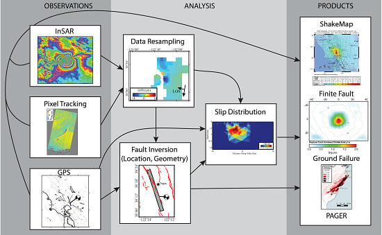
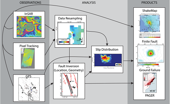
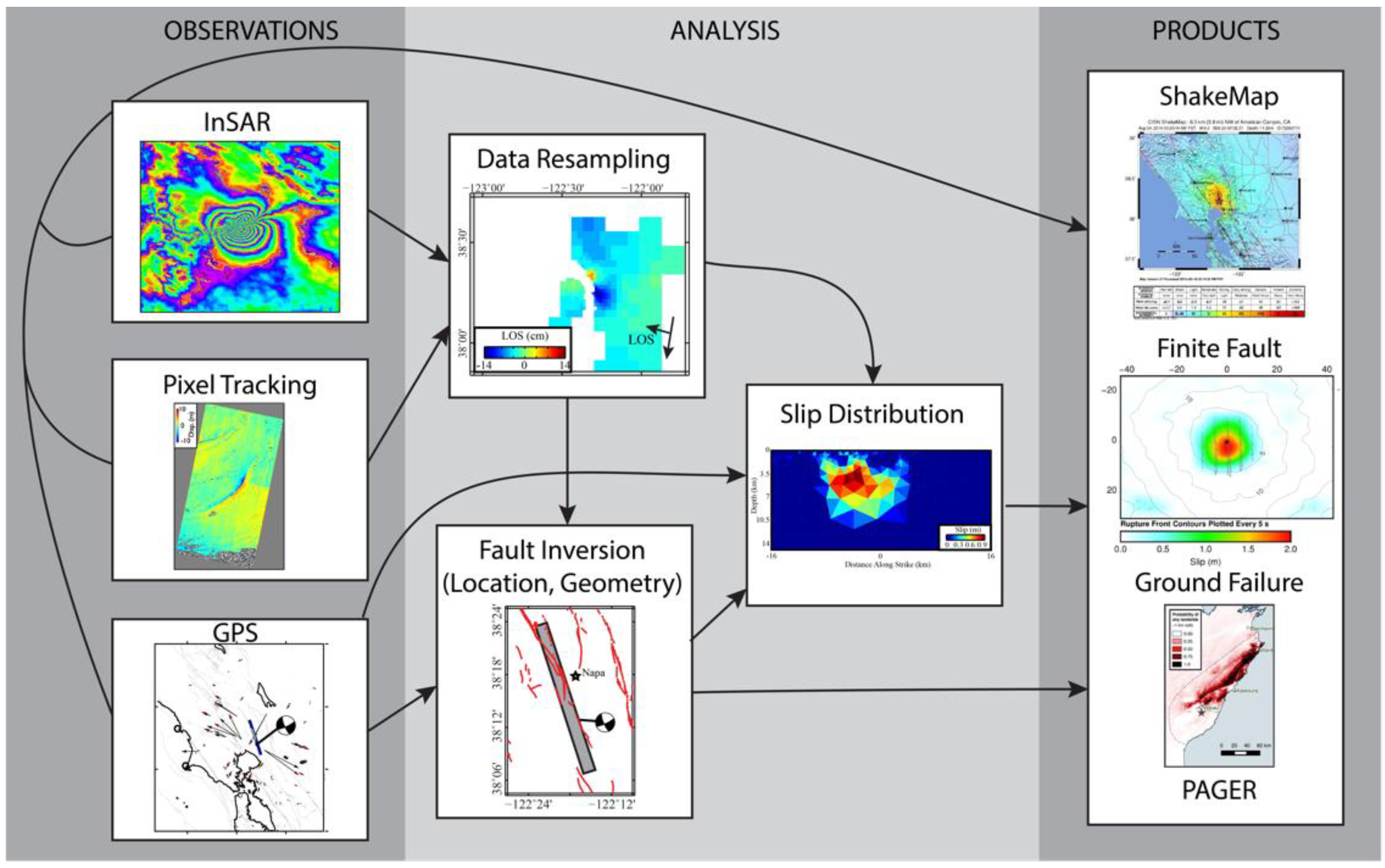
3. Geodetic Response Workflow: Under the Hood

Our workflow for processing and analyzing geodetic observations follows a standard yet opportunistic approach that is updated as necessary depending on available observations and characteristics of the individual earthquakes (Figure 3) [7,8]. Currently, this workflow is not automated. First, we opportunistically collect any available geodetic observations from either continuous GPS stations or satellite imaging platforms. Where GPS observations are available, we extract co-seismic offsets from GPS time series [42] or use rapidly reported co-seismic offsets. We draw GPS time series or offsets from processing facilities (e.g., UNAVCO, the Nevada Geodetic Laboratory [43], ARIA), from network managers such as the Chilean GNSS network [16,44], or from other sources. We generate co-seismic line-of-sight displacements from SAR observations with standard, open source, processing packages (GMTSAR and ISCE) [45,46]. Currently, response with InSAR focuses on processing imagery from the Sentinel-1a/b and ALOS-2 PALSAR-2 sensors, and we expect the forthcoming NISAR L-band mission to continue expanding response capabilities. Prior to Sentinel-1a operations, we used Radarsat-2 and COSMO-SkyMed imagery when available. We have since focused on Sentinel-1 and ALOS-2 imagery because of ease of imagery access and regular image acquisitions. We also generate co-seismic horizontal displacements from optical imagery when feasible using image cross-correlation in the amplitude domain (Figure 2a and Figure 3) (AMPCOR) [47]. Typically, we apply pixel tracking to Landsat-8 panchromatic imagery (15 m spatial resolution) or Sentinel-2 imagery (10 m spatial resolution); however, we also use high-resolution (0.3–0.5 m) commercial optical imagery when available through invocation of the International Disaster Charter.
After deriving surface maps of co-seismic displacement from imaging platforms, we downsample the observations to a computationally tractable number of observations (~103 observations) and estimate the covariance structure of the downsampled dataset [48,49]. Depending on the nature of the earthquake, the full resolution geodetic observations may be used independently, such as a rupture fault trace derived from pixel tracking results (Figure 2a,b and Figure 3). They may additionally be used to manually generate a fault model for distributed slip inversions when there is clear evidence that the earthquake requires greater spatial complexity than a single, planar fault plane. When a fault geometry is not known a-priori or easily parameterized directly from the geodetic observations, we invert the downsampled datasets and/or GPS offsets for the best fitting location (longitude, latitude, and depth) and geometry (strike, dip, rake, and dimensions) of a fault plane with uniform slip using the Neighbourhood Algorithm [50]. Again, this product may be ingested independently into NEIC response products (Figure 2c,d and Figure 3) or used to verify other product inputs. Lastly, after deriving a fault model through manual inspection, from a community dataset (e.g., Slab2.0, SCEC Community Fault Model [51,52], or through an inversion, we invert the available displacements for distributed slip on the fault, with the slip distribution being used to either verify other response products (the teleseismic finite fault model) or inform response products directly (Figure 2e,f and Figure 3) [11,12,13,14]. To derive a slip distribution, we use an approach that iteratively re-discretizes the fault plane with triangles such that the dimensions of individual fault patches reflect the model resolution capability of the inverse problem [53]. This workflow may be repeated several times for a single earthquake as more geodetic observations become available and as the fault model and slip distribution are better refined through additional analysis [7,11] (Figure 3).

4. Case Studies

To date, geodetic observations (GPS, InSAR, and pixel tracking) have contributed to NEIC earthquake response products for a range of earthquakes in different tectonic environments (Figure 1). The nature of contributions of geodesy have varied broadly, from providing independent verification of an earthquake location or teleseismic finite fault model, to independently acting as the source model for shaking and impact products ( Figure 2, Figure 4, Figure 5 and Figure 6). Below, we highlight four case studies where geodetic observations contributed to NEIC earthquake response operations.

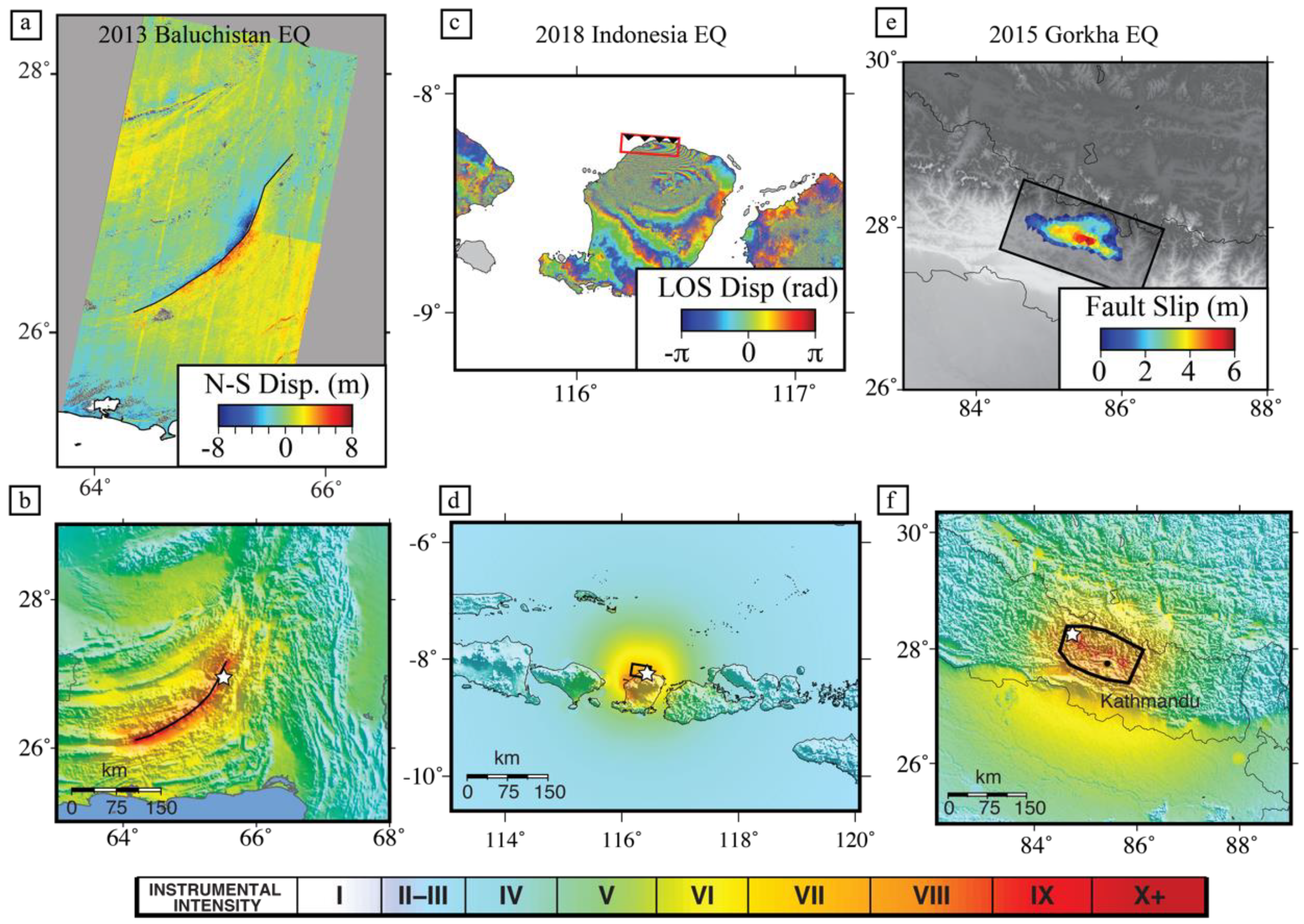
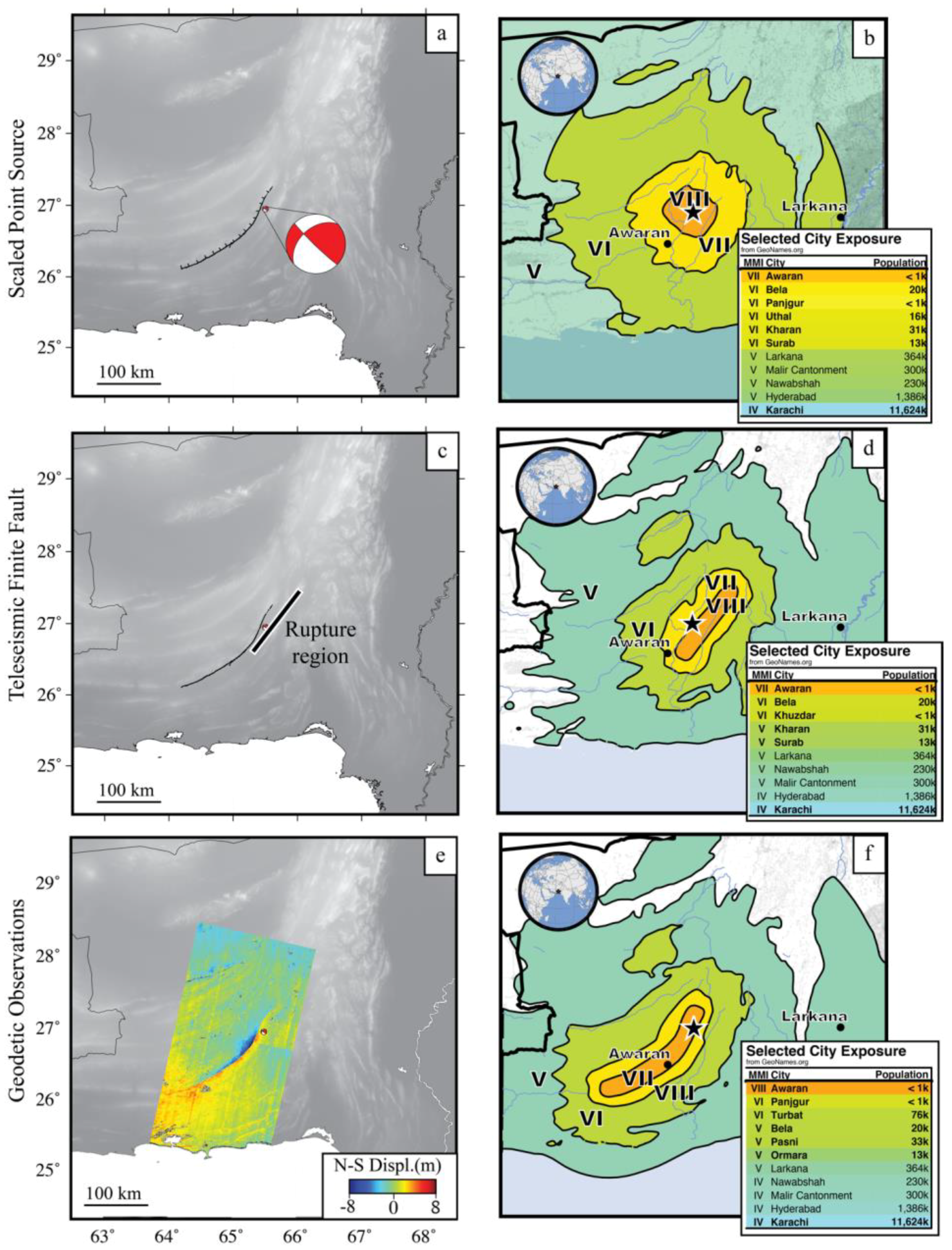
4.1. The 2013 Mw7.7 Baluchistan, Pakistan Earthquake

The 2013 Mw7.7 Baluchistan, Pakistan earthquake (origin time: 24 September 2013, 11:29:47 UTC) was a left-lateral strike slip event that ruptured ~200 km of the Hoshab fault in the Makran accretionary prism of southern Pakistan [13,34,54]. This is the first earthquake for which geodetic imaging observations were directly ingested into NEIC response products in real-time (Figure 4). The earthquake occurred in a relatively sparsely populated region of southern Pakistan, but was notable for the production of large surface displacements exceeding 15 m along portions of the fault in a region where no large upper plate earthquakes were known to have previously occurred [55,56]. Several aspects of this rupture highlight where imaging geodetic observations can provide critical information for earthquake response efforts with respect to the spatial extents of faulting and faulting complexity. First, the earthquake ruptured a single fault with an arcuate fault trace. Rupture initiated in a reach of the fault striking 210° and terminated in a region striking 250°. The USGS W-phase moment tensor solution for the event shows a best-fit strike of 228°. The rupture propagated bilaterally ~150 km to the southwest and ~50 km to the north [13]. The slip was relatively shallow, and likely extended no deeper than ~8 km [13,54]. Second, the earthquake slipped with a primarily left-lateral slip sense and only 4–16% reverse-motion sense on a fault dipping ~60° to the northwest. Moment tensor solutions from different time steps during the rupture suggest that the earthquake retained nearly pure strike–slip motion throughout the rupture duration [54]. The USGS W-phase solution has a best-fit dip of 46° and rake of 6°. Third, the earthquake was initially mislocated ~20 km southeast of the rupture trace [13] at a fixed depth of 15 km.
Figure 4 highlights subsequent iterations of NEIC response products for the Baluchistan earthquake. Here, we illustrate the evolution of response products using PAGER projections population exposure to each Modified Mercalli Intensity (MMI) at selected cities. Initial event response products, released 24 min after origin time, were derived from a scaled point source (Figure 4a–b). The potential accuracy of shaking impacts based on the scaled point source were limited by both the initial mislocation and the lack of information on rupture extent, resulting in an expected broad region of high shaking exposure (MMI VI-VII). Note, however, that the point-source approximation has a larger area of strong shaking about the epicenter than the subsequent finite-fault model ShakeMaps. This is a ramification of ShakeMap’s fault-distance approximation—mentioned earlier—used when the fault is not yet constrained. The average shaking levels are elevated in the epicentral region in an effort to approximate the average overall shaking given the anticipated fault dimensions for the event’s magnitude [28].
The preliminary teleseismic finite fault model, released 1 day after origin time, led to the next major revision of response products. As noted previously, preliminary finite fault models use the event hypocenter, W-phase moment tensor solution, and earthquake scaling relationships to constrain the location and dimensions of the event. In this example, the finite fault model captured the general northeast-southwest trend of the rupture, leading to focusing of high shaking along the same trend and reducing the broader distribution of high shaking predicted by the scaled point source. At the same time, the initial mislocation combined with the as-yet unknown arcuate nature of the rupture led to focusing of high shaking southeast of the mislocated hypocenter along a planar fault. This distribution arose in-part because slip was mapped up-dip of the hypocenter. Moreover, the finite fault model predicted a ~125 km long rupture bilateral rupture that extended expected high shaking exposure toward the northeast (Figure 4c,d).
The first post-event Landsat-8 image was acquired on 26 September 2013, 2 days after origin time (Table 1, Figure 4e,f). Pixel tracking results derived from this acquisition and one on 10 September 2013 revealed many of the rupture characteristics described above, including the arcuate nature of the rupture, the along-strike length of the rupture, and the location of the rupture ~20 km west of the initial hypocenter [13,34,54]. We interpreted a rupture trace from the Landsat-8 pixel tracking results and incorporated this as a line source into ShakeMap, resulting in the final update, released 6.5 days after origin time, of the event products (Figure 4f). This update captured the curved, more westward rupture with predominate moment release southwest of the hypocenter, and resulted in a systematic shift in the location of shaking intensities toward the west/southwest from the teleseismic finite fault model. From the initial scaled point source model to the geodetic model, the overall expected exposure to high shaking (MMI > V) decreased; though, revised impact estimates raised the expected exposure to high shaking in villages such as Awaran (MMI VII to VIII) (Figure 4f).
In many ways, the Baluchistan earthquake highlights an idealized end member example of how geodetic imaging observations can contribute to earthquake response efforts—one in which the observations alone demonstrably improve the accuracy of earthquake response products without the need to model the surface displacement field. The earthquake occurred in a region with few regional seismic observations, which contributed to an initial event mislocation that biased subsequent response products derived from both scaled point sources and teleseismic finite models. Moreover, the earthquake was spatially complex and unusual, rupturing a non-planar fault bilaterally over a distance of ~200 km at relatively shallow depths for a large crustal earthquake. These characteristics are not easily captured by teleseismic finite fault models that include many unknowns that trade-off during an inversion. Accordingly, the geodetic observations provided the most direct constraint on the spatial characteristics of the Baluchistan earthquake without having to undertake any fault source inversions.

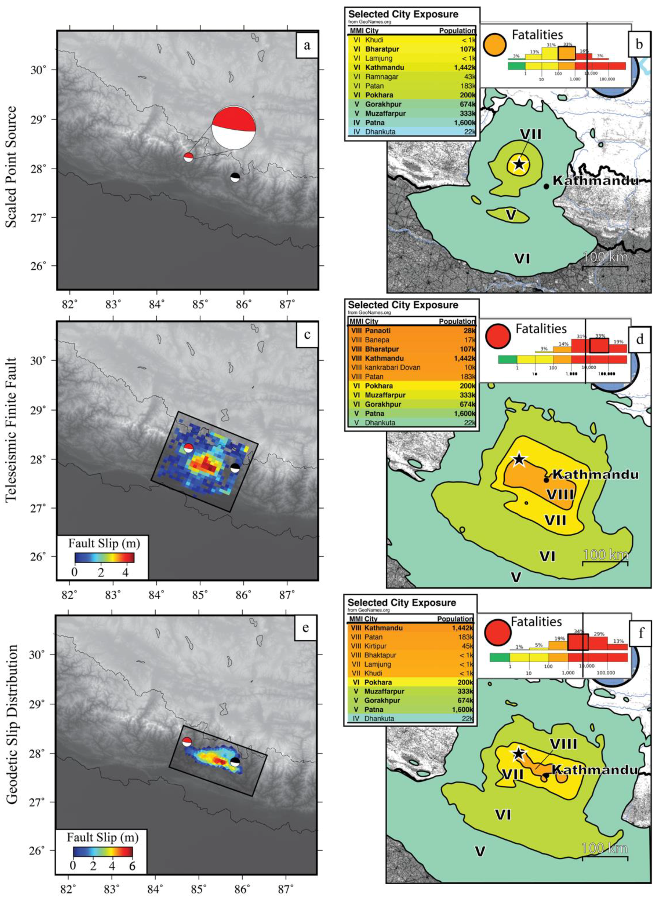
4.2. The 2015 Mw7.8 Gorkha, Nepal Earthquake

The 2015 Mw7.8 Gorkha, Nepal earthquake (origin time: 25 April 2015, 06:11:25) was a thrust-type earthquake that occurred on the Main Himalayan Thrust in central Nepal [11,15,57,58,59]. The earthquake, which originated ~83 km northwest of Kathmandu, rupture unilaterally ~200 km to the east, leading to extensive damage and fatalities (~8,900) from shaking and triggered landslides throughout Nepal (Figure 5). The earthquake was followed on 12 May 2015 by an Mw7.3 aftershock near the Nepalese basecamp of Mt. Everest. Unlike the Baluchistan earthquake, the Gorkha earthquake was entirely blind (buried), so actionable geodetic earthquake source information needed to come from a source model rather than inferred from observations alone. Similarly unlike the Baluchistan earthquake, the preliminary earthquake hypocenter and subsequent teleseismic finite model were accurate when compared to later, more detailed analyses. Accordingly, this case study highlights the importance of rupture finiteness in NEIC response products and how geodetic observations can help to refine teleseismic finite fault models to produce an ultimately more accurate projection of earthquake impacts.
The most noticeable disparity in earthquake response products for the Gorkha earthquake is between those governed by a scaled point source, first released 22 min after origin time, and those governed by a finite source, first released 4 h after origin time (Figure 5). In the preliminary scaled point source solution, PAGER and ShakeMap products focused anticipated shaking around the event hypocenter 83 km northwest of Kathmandu and in west-central Nepal. Understandably, the scaled point source solution did not capture the eastward rupture propagation beneath Kathmandu, and the preliminary response level (“Orange alert”, 10–1000 fatalities) indicated a nation-scale impact and response level event (Figure 5a,b). Following publication of the teleseismic finite fault model that captured the eastward rupture and proximity of slip to Kathmandu, the PAGER alert level rose to “Red” with an anticipated number of fatalities of 10,000–100,000 (Figure 5c,d).
Preliminary co-seismic displacements from GPS of the Gorkha earthquake were provided by the NASA ARIA group on April 27 (origin time +2 days). These were followed by the releases of co-seismic Sentinel-1 interferograms by the COMET research group on 29 April and 30 April (4 and 5 days after origin time), and ALOS-2 ScanSAR interferograms on 28 April (3 days after origin time) and 3 May (8 days after origin time), respectively, by UC San Diego [59]. Each of these data sets (GPS and downsampled interferograms) were inverted simultaneously for both the location and geometry of the causative fault, and the spatial distribution of fault slip (Figure 5e) [11]. This slip distribution constrained the up-dip limit of fault slip to be deeper than that imaged in the teleseismic finite fault model, but largely confirmed the along-strike length of the rupture. The spatial constraints from InSAR were used to re-parameterize the teleseismic finite fault model that was then ingested into ShakeMap. This final iteration, released 9 days after origin time, retained the “Red” alert level, but it condensed the region of highest shaking and changed the highest probability of fatalities to the range (1000–10,000) that ultimately bore true. Although the information gained from geodetic observations did not systematically change the nature of NEIC response products as they did for the Baluchistan earthquake, the geodetic observations served to provide a verification and refinement of an already well-constrained earthquake source model. This feedback relationship in turn led to a more accurate characterization of the human impacts of the Gorkha earthquake.

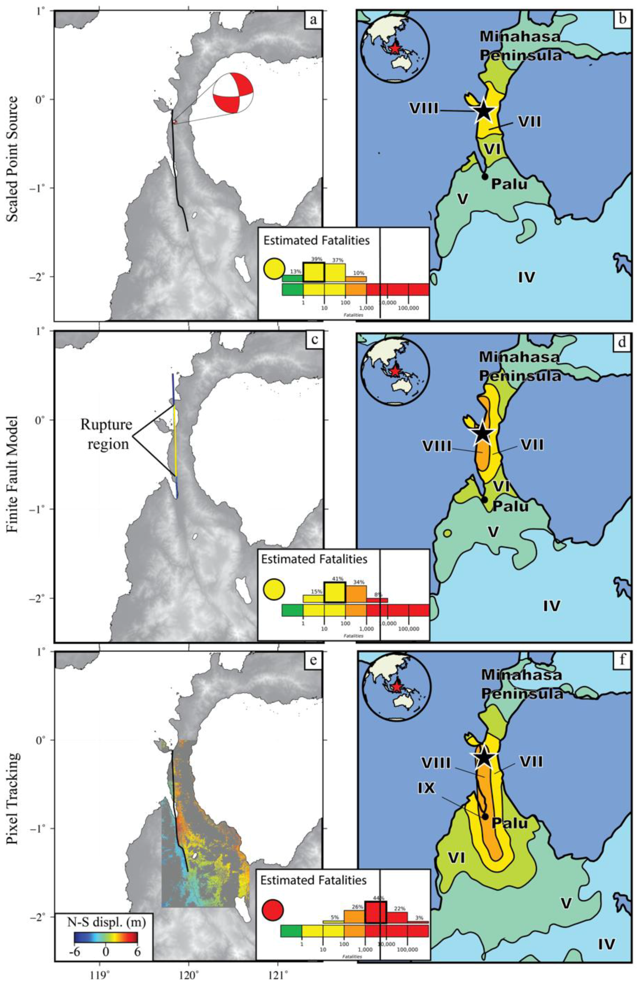
4.3. The 2018 Mw7.5 Palu, Indonesia Earthquake

The 2018 Mw7.5 Palu, Indonesia earthquake (origin time: 28 September 2018, 10:02:45) was a left-lateral strike slip earthquake that occurred on the island of Sulawesi along the Palu-Koro fault (Figure 6) [60,61]. This earthquake was notable for several reasons. First, it ruptured both through the city of Palu (population 282,000) and the southernmost end of Palu Bay where a tsunami was triggered by co-seismic landslides. The earthquake nucleated on the Minahasa Peninsula and propagated unilaterally to the south towards and through Palu (Figure 6). Second, the earthquake rupture propagated at supershear velocities of ~4.1 km/s [60,61]. Rupture velocity can be solved for in teleseismic finite fault models, though teleseismic data is typically fairly insensitive to this parameter, which trades off with other aspects of the fault model. In the NEIC’s rapid fault modeling workflow, rupture velocity is usually allowed to vary over a range of ~1.5–3.5 km/s, from an average starting velocity of 2.5 km/s. This limited range helps to reduce the total number of model parameters in the inversion search space. Rupture velocities that fall outside of this range, such as during a supershear rupture or slow rupturing tsunamigenic earthquakes, can in turn lead to a mischaracterization of the total ruptured fault length while still fitting teleseismic waveforms. For example, the source duration of the Palu earthquake was ~26 s. With a rupture velocity of 2.5 km/s, this would result in a ~65 km long rupture and rupture termination without passing through Palu. In contrast, a rupture velocity of 4.1 km/s would result in a ~107 km rupture that ended after passing past Palu.
As in the Gorkha earthquake case study, the USGS NEIC preliminary location accurately captured the hypocenter of the earthquake. Preliminary shaking and impact estimates from the scaled point source solution, released 20 min after origin time, placed the highest impacts 70–80 km north of Palu on the Minahasa Peninsula, resulting in an “Yellow” alert level and relatively modest expected impacts in the city (Figure 6a,b). The first finite fault model, released ~3 h after origin time, captured the southward propagation of the earthquake, resulting in the expansion of the region of expected high impacts further south (Figure 6c,d). However, the finite fault model did not extend slip as far south as Palu because a fast rupture velocity was not required by the teleseismic data. Impact projections from this model retained the “Yellow” alert level and modest impacts in Palu.
Pixel tracking results from Landsat-8 and Sentinel-2 imagery acquired on 2 October 2018, 3 days, 16 h after origin time, revealed the full ~130 km long extent of the Palu earthquake (Figure 6e) [60,61]. The geodetic imaging results showed that the rupture propagated southward along the Minahasa Peninsula as a blind event before stepping to the west beneath Palu Bay and rupturing directly through Palu. The earthquake ruptured the surface through Palu with offsets of 5–6 m (Figure 6e). The surface rupture then continued south of Palu through a left-stepping bend before terminating 47 km south of Palu (Figure 6e). The pixel tracking results and a later Sentinel-1 interferogram confirmed the northern extent of the rupture constrained in the teleseismic finite fault model. Similar to the Baluchistan earthquake, we extracted a line source from the pixel tracking results that was then incorporated into ShakeMap and released 4.5 days after origin time (Figure 6f). Inclusion of the southern extent of the rupture through Palu increased the PAGER alert level to “Red” since it then captured the expected high shaking exposure in Palu (Figure 6e,f).

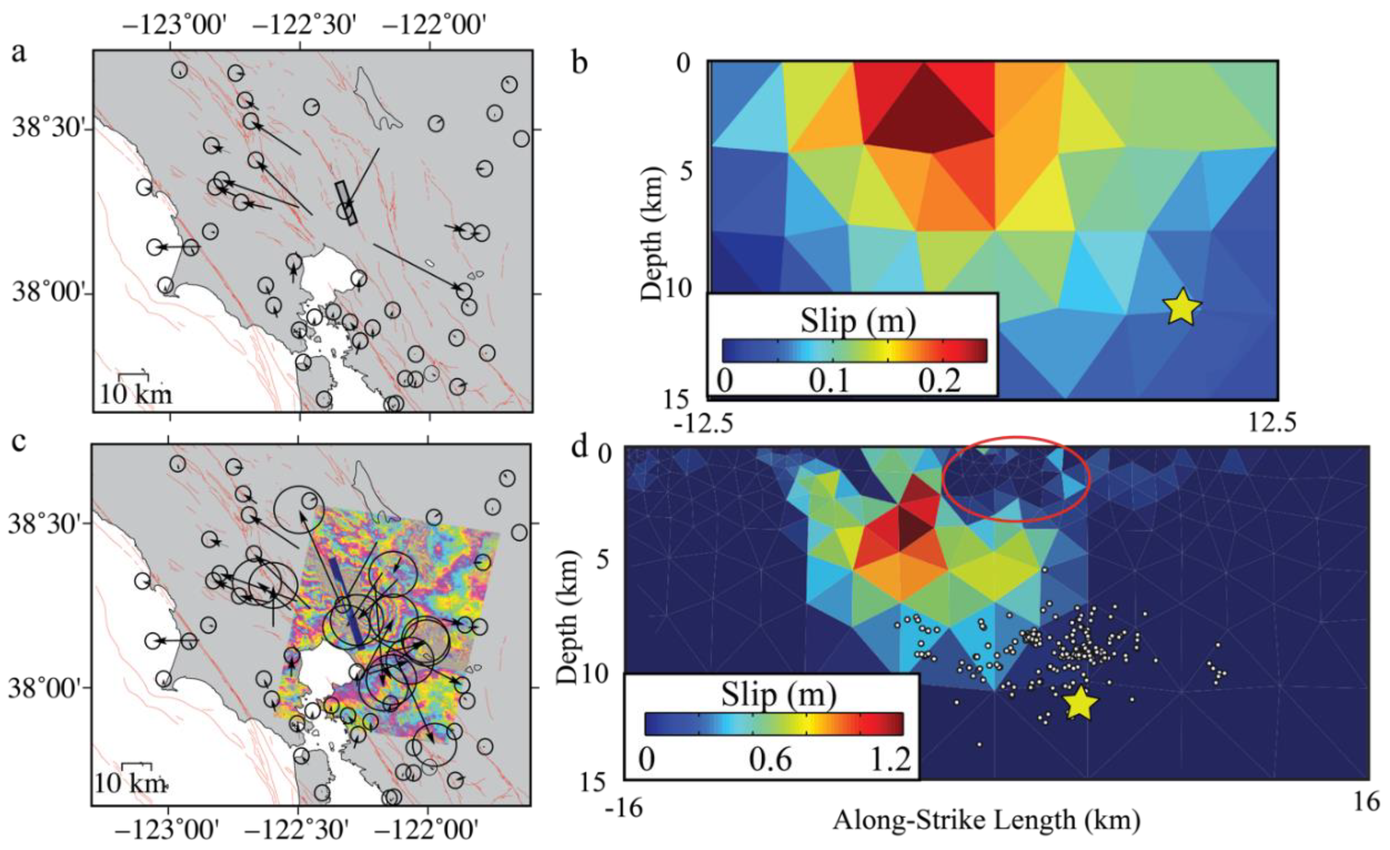
4.4. The 2014 Mw6.0 South Napa, California Earthquake

The 2014 Mw6.0 South Napa, California earthquake (24 August 2014, 10:20:44) was a strike-slip event that occurred on the West Napa Fault within the broader San Andreas Fault system [7,8]. Unlike the previous earthquakes highlighted in this paper, the South Napa earthquake occurred within a dense local and regional network of seismometers and strong ground motion instruments that provided direct shaking observations for ShakeMap [8,62]. In addition, well-recorded aftershocks and a finite fault model derived from local seismic observations provided rapid finite source constraints [8,63]. Consequently, geodetic observations provided limited input for NEIC operational response products other than to verify the location and spatial extent of the fault source. Geodetic observations, however, provided improved operational awareness for ground support teams investigating the distribution of surface rupture and ground failure [8,64] and an increasingly well constrained source model in the hours to days following the earthquake [7] (Figure 7). Within 24 h of origin time, we produced a co-seismic fault model and slip distribution from continuous GPS stations operating in the San Francisco Bay area (Figure 7a,b). This model was updated the following day with an additional day of continuous GPS observations and disseminated internally within the USGS and on the NEIC event response page [7]. Six days after the earthquake, the NASA ARIA group released a co-seismic COSMO-SkyMed interferogram that was used to update our source model again (Figure 7c) [7]. The addition of spatially dense InSAR observations demonstrably improved the resolution of the slip distribution, resulting in a more detailed model of fault slip that defined regions with and without co-seismic surface rupture (Figure 7c,d). Notably, the shallow region up-dip of co-seismic slip that did not slip during the earthquake (Figure 7c) was the locus of subsequent surface slip associated with post-seismic afterslip [65,66,67]. Offset fringe patterns in the COSMO-SkyMed interferogram also helped ground teams identify additional surface ruptures that were not located along the main rupture trace [8,64].
The South Napa earthquake example highlights two important contributions imaging geodetic observations make to earthquake response efforts. Co-seismic GPS observations were available in near real-time for this event (Figure 7a) [68]; however, these observations could only contribute to a low-resolution estimate of fault slip despite the dense network (Figure 7a,b). InSAR observations combined with GPS observations in turn were critical to imaging the spatially complex distribution of fault slip (Figure 7c,d). Although this capability contributed little new information in densely instrumented portions of California, similar observations and modeling efforts applied to moderate magnitude earthquakes elsewhere in the world (e.g., the 2003 M6.6 Bam, Iran earthquake) could prove critical in characterizing the rupture details of the earthquake. Rapidly acquired InSAR observations further provided a means to identify surface rupture in unmapped regions, and how these might evolve with early surface creep from afterslip to impact local infrastructure [64].

5. Conclusions

Ground based and remotely sensed geodetic observations of earthquakes have the power to contribute important and independent constraints for global operational earthquake response [7,9,11,37,69]. These contributions span the spectrum of providing an independent verification of seismically-derived earthquake source parameters (e.g., the 2014 South Napa, California earthquake, Figure 7) to independently constraining earthquake response products (e.g., the 2013 Baluchistan, Pakistan earthquake, Figure 4) by providing much more robust estimates of the faulting extent than seismic data alone. Imaging geodesy observations (InSAR, pixel tracking) in particular are a critical component of these efforts given that they afford greater resolution of earthquake slip processes across a range of earthquake magnitudes (M5+) than GPS or seismological observations alone, and their resolution capabilities are effectively constant anywhere in the world when imagery is coherent, including where GPS networks are non-existent or seismological observations are sparse. A long-standing limitation of the application of geodesy in earthquake response was the infrequent acquisition and limited access of satellite images; however, new (Sentinel-1, ALOS-2) satellite missions have systematically increased the frequency of image acquisitions such that geodetic earthquake response is tractable on the response timescales for many significant global earthquakes (Figure 1). Forthcoming missions (NISAR) will continue to improve these capabilities.
There remain limitations to incorporating geodetic observations in operational earthquake response efforts, but these limitations are increasingly mitigated by the large volume and diversity of remote sensing images acquired, and continuing efforts to develop earthquake analysis infrastructure. First, these approaches are only applicable when an earthquake deforms the land surface (e.g., continental and subduction zone earthquakes), and when the earthquake is sufficiently large and/or shallow enough to produce resolvable surface displacements. This limits the applicability of geodetic observations to relatively shallow and moderate to large magnitude earthquakes that occur on or proximal to land. These events are often the most impactful to society, but geodetic observations will not be applicable in all earthquake scenarios. Second, remote sensing geodetic observations will continue to be susceptible to issues associated with image decorrelation—particularly in highly vegetated regions [10]—cloud cover in optical imagery, and SAR look angles. For example, Sentinel-1 observations were acquired within one day of the Mw6.1 22 April 2019 Philippines earthquake on the island of Luzon. However, the strike-slip rupture was parallel to the SAR orbit direction, and the InSAR results were insensitive to the surface deformation. The volumes of images acquired from different viewing geometries and different imaging approaches, though, improve the probability of “capturing” any given earthquake despite these issues. Moreover, the forthcoming NISAR mission, which includes an L-band radar, will improve on Sentinel-1 (a C-band radar) capabilities to image surface deformation in more surface environments. Third, as mentioned previously, geodetic image processing and analysis is not automated at the NEIC. The current requirement that a researcher or group of researchers manually access, process, and model the remote sensing observations can lead to delays in the production of response products beyond the shortening time latency of image acquisitions and/or computation time needed for processing and analysis. Future efforts at the NEIC, such as the proposed development of the Geodetic Centroid (GCent) Platform [7], will enable more automated and more systematic analysis of geodetic data sets and reduce this limitation. Last, there remains a time gap between an earthquake and the availability of most geodetic observations that is longer than what is typical of seismic observations. The average time to first acquisition since the launch of Sentinel is <3 days, and has been as short as 1 h for events we have assessed (Table 1). While acquisition frequency has improved dramatically since 2014 and will continue to do so with NISAR, InSAR and optical correlation-calibrated response products will likely continue to be released on timescales of days after origin time, rather than minutes to hours. Accordingly, geodetic observations stand as one component in a multi-faceted approach to providing accurate and timely information for earthquake response.

Author Contributions

W.D.B. conducted the geodetic analysis and fault model inversions; G.P.H. conducted the teleseismic finite fault inversions. All authors participated in discussing and editing the manuscript.

Funding

This research was funded in part by a U.S. Geological Survey Mendenhall and postdoctoral fellowship and a U.S. Geological Survey Intragovernmental Personnel Agreement.

Acknowledgments

The author thanks many individuals who provided earthquake observations from satellite and GPS observations in the days following catastrophic events. The authors also thank the three anonymous reviewers and Ryan Gold, whose suggestions helped improve the quality of this manuscript. Pre-processed InSAR imagery (Sentinel-1, ALOS-2, Radarsat-2, and COSMO-SkyMed) used in events detailed in Table 1 originated from multiple sources: Natural Resources Canada (Sergey Samsonov), U.C. San Diego, the NASA ARIA group, and the UK COMET-LiCS group. Sentinel-1 imagery processed by the co-authors was acquired from the Alaska Satellite Facility DAAC and the ESA SciHub repository; ALOS-2 imagery processed by the co-authors was acquired through a JAXA science PI data agreement. Sentinel-2 imagery was acquired from the ESA SciHub repository; Landsat-8 imagery was acquired from the USGS EarthExplorer repository. Co-seismic GPS offsets and GPS time series were acquired and/or processed from the NASA ARIA group, the Chilean GNSS network, the USGS, and the University of Nevada, Reno Geodesy Laboratory. Several figures were generated with the Generic Mapping Tool [70]. W.D. Barnhart was funded in part by a USGS Mendenhall postdoctoral fellowship and a USGS Intergovernmental Personnel Agreement.

Conflicts of Interest

The authors declare no conflict of interest.

References

  1. Hayes, G.P. Rapid source characterization of the 2011 Mw 9.0 off the Pacific coast of Tohoku Earthquake. Earth Planets Space 2011, 63, 529–534. [Google Scholar] [CrossRef]
  2. Wald, D.J.; Jaiswal, K.S.; Marano, K.D.; Bausch, D. Earthquake Impact Scale. Nat. Hazards Rev. 2011, 12, 125–139. [Google Scholar] [CrossRef] [Green Version]
  3. Wald, D.J.; Quitoriano, V.; Heaton, T.H.; Kanamori, H.; Scrivner, C.W.; Worden, C.B. TriNet “ShakeMaps”: Rapid Generation of Peak Ground Motion and Intensity Maps for Earthquakes in Southern California. Earthq. Spectra 1999, 15, 537–555. [Google Scholar] [CrossRef]
  4. Wald, D.J.; Jaiswal, K.S.; Marano, K.D.; Bausch, D.B.; Hearne, M.G. PAGER—Rapid Assessment of an Earthquake’s Impact; USGS Fact Sheet; U.S. Geological Survey: Reston, VA, USA, 2010.
  5. Allstadt, K.E.; Thompson, E.M.; Hearne, M.; Jessee, M.A.N.; Zhu, J.; Wald, D.J.; Tanyas, H. Integrating landslide and liquefaction hazard and loss estimates with existing USGS real-time earthquake information products. In Proceedings of the 16th World Conference on Earthquake Engineering, Santiago, Chile, 9–13 January 2017. [Google Scholar]
  6. van der Elst, N.J.; Page, M.T. Nonparametric Aftershock Forecasts Based on Similar Sequences in the Past. Seismol. Res. Lett. 2018, 89, 145–152. [Google Scholar] [CrossRef]
  7. Barnhart, W.D.; Murray, J.R.; Yun, S.-H.; Svarc, J.L.; Samsonov, S.V.; Fielding, E.J.; Brooks, B.A.; Milillo, P. Geodetic Constraints on the 2014 M 6.0 South Napa Earthquake. Seismol. Res. Lett. 2015, 86, 335–343. [Google Scholar] [CrossRef] [Green Version]
  8. Brocher, T.M.; Baltay, A.S.; Hardebeck, J.L.; Pollitz, F.F.; Murray, J.R.; Llenos, A.L.; Schwartz, D.P.; Blair, J.L.; Ponti, D.J.; Lienkaemper, J.J.; et al. The M6. 0 24 August 2014 South Napa Earthquake. Seismol. Res. Lett. 2015, 86, 309–326. [Google Scholar]
  9. Elliott, J.R.; Walters, R.J.; Wright, T.J. The role of space-based observation in understanding and responding to active tectonics and earthquakes. Nat. Commun. 2016, 7, 13844. [Google Scholar] [CrossRef] [PubMed] [Green Version]
  10. Funning, G.J.; Garcia, A. A systematic study of earthquake detectability using Sentinel-1 Interferometric Wide-Swath data. Geophys. J. Int. 2019, 216, 332–349. [Google Scholar] [CrossRef]
  11. Hayes, G.P.; Briggs, R.W.; Barnhart, W.D.; Yeck, W.L.; McNamara, D.E.; Wald, D.J.; Nealy, J.L.; Benz, H.M.; Gold, R.D.; Jaiswal, K.S.; et al. Rapid Characterization of the 2015 Mw 7.8 Gorkha, Nepal, Earthquake Sequence and Its Seismotectonic Context. Seismol. Res. Lett. 2015, 86, 1557–1567. [Google Scholar] [CrossRef]
  12. Barnhart, W.D.; Hayes, G.P.; Samsonov, S.V.; Fielding, E.J.; Seidman, L.E. Breaking the oceanic lithosphere of a subducting slab: The 2013 Khash, Iran earthquake. Geophys. Res. Lett. 2014, 41, 32–36. [Google Scholar] [CrossRef]
  13. Barnhart, W.D.; Hayes, G.P.; Briggs, R.W.; Gold, R.D.; Bilham, R. Ball-and-socket tectonic rotation during the 2013 Balochistan earthquake. Earth Planet. Sci. Lett. 2014, 403, 210–216. [Google Scholar] [CrossRef]
  14. Hayes, G.P.; Herman, M.W.; Barnhart, W.D.; Furlong, K.P.; Riquelme, S.; Benz, H.M.; Bergman, E.; Barrientos, S.; Earle, P.S.; Samsonov, S. Continuing megathrust earthquake potential in Chile after the 2014 Iquique earthquake. Nature 2014, 512, 295–299. [Google Scholar] [CrossRef] [PubMed]
  15. McNamara, D.E.; Yeck, W.L.; Barnhart, W.D.; Schulte-Pelkum, V.; Bergman, E.; Adhikari, L.B.; Dixit, A.; Hough, S.E.; Benz, H.M.; Earle, P.S. Source modeling of the 2015 Mw 7.8 Nepal (Gorkha) earthquake sequence: Implications for geodynamics and earthquake hazards. Tectonophysics 2017, 714–715, 21–30. [Google Scholar] [CrossRef]
  16. Barnhart, W.D.; Murray, J.R.; Briggs, R.W.; Gomez, F.; Miles, C.P.J.; Svarc, J.; Riquelme, S.; Stressler, B.J. Coseismic slip and early afterslip of the 2015 Illapel, Chile, earthquake: Implications for frictional heterogeneity and coastal uplift. J. Geophys. Res. Solid Earth 2016, 121, 6172–6191. [Google Scholar] [CrossRef] [Green Version]
  17. Herman, M.W.; Nealy, J.L.; Yeck, W.L.; Barnhart, W.D.; Hayes, G.P.; Furlong, K.P.; Benz, H.M. Integrated geophysical characteristics of the 2015 Illapel, Chile, earthquake. J. Geophys. Res. Solid Earth 2017, 122, 4691–4711. [Google Scholar] [CrossRef]
  18. Yeck, W.L.; Hayes, G.P.; McNamara, D.E.; Rubinstein, J.L.; Barnhart, W.D.; Earle, P.S.; Benz, H.M. Oklahoma experiences largest earthquake during ongoing regional wastewater injection hazard mitigation efforts. Geophys. Res. Lett. 2017, 44, 711–717. [Google Scholar] [CrossRef]
  19. Barnhart, W.D.; Yeck, W.L.; McNamara, D.E. Induced earthquake and liquefaction hazards in Oklahoma, USA: Constraints from InSAR. Remote Sens. Environ. 2018, 218, 1–12. [Google Scholar] [CrossRef]
  20. Barnhart, W.D.; Brengman, C.M.J.; Li, S.; Peterson, K.E. Ramp-flat basement structures of the Zagros Mountains inferred from co-seismic slip and afterslip of the 2017 Mw7.3 Darbandikhan, Iran/Iraq earthquake. Earth Planet. Sci. Lett. 2018, 496, 96–107. [Google Scholar] [CrossRef]
  21. Nissen, E.; Ghods, A.; Karasözen, E.; Elliott, J.R.; Barnhart, W.D.; Bergman, E.A.; Hayes, G.P.; Jamal-Reyhani, M.; Nemati, M.; Tan, F.; et al. The 12 November 2017 Mw 7.3 Ezgeleh-Sarpolzahab (Iran) Earthquake and Active Tectonics of the Lurestan Arc. J. Geophys. Res. Solid Earth 2019, 124, 2124–2152. [Google Scholar] [CrossRef]
  22. Guy, M.R.; Patton, J.M.; Fee, J.; Hearne, M.; Martinez, E.; Ketchum, D.; Worden, C.; Quitoriano, V.; Hunter, E.; Smoczyk, G.; et al. National Earthquake Information Center Systems Overview and Integration; Open-File Report; U.S. Geological Survey: Reston, VA, USA, 2015; p. 28.
  23. Hayes, G.P. The finite, kinematic rupture properties of great-sized earthquakes since 1990. Earth Planet. Sci. Lett. 2017, 468, 94–100. [Google Scholar] [CrossRef]
  24. Wald, D.J.; Franco, G. Financial Decision-Making Based on Near–Real-Time Earthquake Information. In Proceedings of the 16th World Conference on Earthquake Engineering, Santiago, Chile, 9–13 January 2017. [Google Scholar]
  25. Worden, C.B.; Wald, D.J. Shakemap Manual Online: Technical Manual, User’s Guide, and Software Guide; U.S. Geological Survey: Reston, VA, USA, 2016.
  26. Wald, D.J.; Allen, T.I. Topographic Slope as a Proxy for Seismic Site Conditions and Amplification. Bull. Seismol. Soc. Am. 2007, 97, 1379–1395. [Google Scholar] [CrossRef] [Green Version]
  27. Worden, C.B.; Gerstenberger, M.C.; Rhoades, D.A.; Wald, D.J. Probabilistic Relationships between Ground-Motion Parameters and Modified Mercalli Intensity in California. Bull. Seismol. Soc. Am. 2012, 102, 204–221. [Google Scholar] [CrossRef]
  28. Thompson, E.M.; Worden, C.B. Estimating Rupture Distances without a RuptureEstimating Rupture Distances without a Rupture. Bull. Seismol. Soc. Am. 2018, 108, 371–379. [Google Scholar] [CrossRef]
  29. Avouac, J.-P.; Ayoub, F.; Leprince, S.; Konca, O.; Helmberger, D.V. The 2005, Mw 7.6 Kashmir earthquake: Sub-pixel correlation of ASTER images and seismic waveforms analysis. Earth Planet. Sci. Lett. 2006, 249, 514–528. [Google Scholar] [CrossRef] [Green Version]
  30. Fialko, Y.; Simons, M.; Agnew, D. The complete (3-D) surface displacement field in the epicentral area of the 1999 MW7.1 Hector Mine Earthquake, California, from space geodetic observations. Geophys. Res. Lett. 2001, 28, 3063–3066. [Google Scholar] [CrossRef]
  31. Funning, G.J.; Parsons, B.; Wright, T.J.; Jackson, J.A.; Fielding, E.J. Surface displacements and source parameters of the 2003 Bam (Iran) earthquake from Envisat advanced synthetic aperture radar imagery. J. Geophys. Res. Solid Earth 2005, 110, 1–23. [Google Scholar] [CrossRef]
  32. Hamling, I.J.; Hreinsdóttir, S.; Clark, K.; Elliott, J.; Liang, C.; Fielding, E.; Litchfield, N.; Villamor, P.; Wallace, L.; Wright, T.J.; et al. Complex multifault rupture during the 2016 Mw 7.8 Kaikōura earthquake, New Zealand. Science 2017, 356, 1–10. [Google Scholar] [CrossRef] [PubMed]
  33. Massonnet, D.; Rossi, M.; Carmona, C.; Adragna, F.; Peltzer, G.; Feigl, K.; Rabaute, T. The displacement field of the Landers earthquake mapped by radar interferometry. Nature 1993, 364, 138–142. [Google Scholar] [CrossRef]
  34. Avouac, J.-P.; Ayoub, F.; Wei, S.; Ampuero, J.-P.; Meng, L.; Leprince, S.; Jolivet, R.; Duputel, Z.; Helmberger, D. The 2013, Mw 7.7 Balochistan earthquake, energetic strike-slip reactivation of a thrust fault. Earth Planet. Sci. Lett. 2014, 391, 128–134. [Google Scholar] [CrossRef] [Green Version]
  35. Simons, M.; Fialko, Y.; Rivera, L. Coseismic Deformation from the 1999 Mw 7.1 Hector Mine, California, Earthquake as Inferred from InSAR and GPS Observations. Bull. Seismol. Soc. Am. 2002, 92, 1390–1402. [Google Scholar] [CrossRef]
  36. Sudhaus, H.; Jónsson, S. Source model for the 1997 Zirkuh earthquake (MW = 7.2) in Iran derived from JERS and ERS InSAR observations. Geophys. J. Int. 2011, 185, 676–692. [Google Scholar] [CrossRef]
  37. Owen, S.E.; Fielding, E.J.; Yun, S.H.; Yue, H.; Polet, J.; Riel, B.V.; Liang, C.; Huang, M.H.; Webb, F.; Simons, M.; et al. The Advanced Rapid Imaging and Analysis (ARIA) Project’s Response to the April 25, 2015 M7.8 Nepal Earthquake: Rapid Measurements and Models for Science and Situational Awareness. In Proceedings of the AGU Fall Meeting, San Francisco, CA, USA, 14–18 December 2015. [Google Scholar]
  38. Barnhart, W.D.; Lohman, R.B.; Mellors, R.J. Active accommodation of plate convergence in Southern Iran: Earthquake locations, triggered aseismic slip, and regional strain rates. J. Geophys. Res. Solid Earth 2013, 118, 5699–5711. [Google Scholar] [CrossRef]
  39. Ferreira, A.M.G.; Weston, J.; Funning, G.J. Global compilation of interferometric synthetic aperture radar earthquake source models: 2. Effects of 3-D Earth structure. J. Geophys. Res. Solid Earth 2011, 116, 1–21. [Google Scholar] [CrossRef]
  40. Lohman, R.B.; Simons, M. Locations of selected small earthquakes in the Zagros mountains. Geochem. Geophys. Geosystems 2005, 6, 1–10. [Google Scholar] [CrossRef]
  41. Weston, J.; Ferreira, A.M.G.; Funning, G.J. Global compilation of interferometric synthetic aperture radar earthquake source models: 1. Comparisons with seismic catalogs. J. Geophys. Res. Solid Earth 2011, 116, 1–20. [Google Scholar] [CrossRef]
  42. Langbein, J.; Murray, J.R.; Snyder, H.A. Coseismic and Initial Postseismic Deformation from the 2004 Parkfield, California, Earthquake, Observed by Global Positioning System, Electronic Distance Meter, Creepmeters, and Borehole Strainmeters. Bull. Seismol. Soc. Am. 2006, 96, S304–S320. [Google Scholar] [CrossRef]
  43. Blewitt, G.; Hammond, W.C.; Kremer, C. Harnessing the GPS data explosion for interdisciplinary science. Eos Trans. Am. Geophys. Union 2018, 99. [Google Scholar] [CrossRef]
  44. Báez, J.C.; Leyton, F.; Troncoso, C.; del Campo, F.; Bevis, M.; Vigny, C.; Moreno, M.; Simons, M.; Kendrick, E.; Parra, H.; et al. The Chilean GNSS Network: Current Status and Progress toward Early Warning Applications. Seismol. Res. Lett. 2018, 89, 1546–1554. [Google Scholar] [CrossRef]
  45. Rosen, P.A.; Gurrola, E.; Sacco, G.F.; Zebker, H. The InSAR scientific computing environment. In Proceedings of the EUSAR 2012; 9th European Conference on Synthetic Aperture Radar, Nuremberg, Germany, 23–26 April 2012; pp. 730–733. [Google Scholar]
  46. Sandwell, D.; Mellors, R.; Tong, X.; Wei, M.; Wessel, P. Open radar interferometry software for mapping surface Deformation. Eos Trans. Am. Geophys. Union 2011, 92, 234. [Google Scholar] [CrossRef]
  47. Rosen, P.A.; Hensley, S.; Peltzer, G.; Simons, M. Updated repeat orbit interferometry package released. Eos Trans. Am. Geophys. Union 2004, 85, 47. [Google Scholar] [CrossRef]
  48. Lohman, R.B.; Simons, M. Some thoughts on the use of InSAR data to constrain models of surface deformation: Noise structure and data downsampling. Geochem. Geophys. Geosystems 2005, 6, 1–12. [Google Scholar] [CrossRef]
  49. Lohman, R.B.; Barnhart, W.D. Evaluation of earthquake triggering during the 2005-2008 earthquake sequence on Qeshm Island, Iran. J. Geophys. Res. Solid Earth 2010, 115, 1–13. [Google Scholar] [CrossRef]
  50. Sambridge, M. Geophysical inversion with a neighbourhood algorithm—I. Searching a parameter space. Geophys. J. Int. 1999, 138, 479–494. [Google Scholar] [CrossRef]
  51. Hayes, G.P.; Moore, G.L.; Portner, D.E.; Hearne, M.; Flamme, H.; Furtney, M.; Smoczyk, G.M. Slab2, a comprehensive subduction zone geometry model. Science 2018, 362, 58–61. [Google Scholar] [CrossRef] [PubMed]
  52. Plesch, A.; Shaw, J.H.; Benson, C.; Bryant, W.A.; Carena, S.; Cooke, M.; Dolan, J.; Fuis, G.; Gath, E.; Grant, L.; et al. Community Fault Model (CFM) for Southern CaliforniaCommunity Fault Model (CFM) for Southern California. Bull. Seismol. Soc. Am. 2007, 97, 1793–1802. [Google Scholar] [CrossRef]
  53. Barnhart, W.D.; Lohman, R.B. Automated fault model discretization for inversions for coseismic slip distributions. J. Geophys. Res. Solid Earth 2010, 115, 1–17. [Google Scholar] [CrossRef]
  54. Jolivet, R.; Duputel, Z.; Riel, B.; Simons, M.; Rivera, L.; Minson, S.E.; Zhang, H.; Aivazis, M.A.G.; Ayoub, F.; Leprince, S.; et al. The 2013 Mw 7.7 Balochistan Earthquake: Seismic Potential of an Accretionary Wedge. Bull. Seismol. Soc. Am. 2014, 104, 1020–1030. [Google Scholar] [CrossRef] [Green Version]
  55. Barnhart, W.D.; Briggs, R.W.; Reitman, N.G.; Gold, R.D.; Hayes, G.P. Evidence for slip partitioning and bimodal slip behavior on a single fault: Surface slip characteristics of the 2013 Mw7.7 Balochistan, Pakistan earthquake. Earth Planet. Sci. Lett. 2015, 420, 1–11. [Google Scholar] [CrossRef]
  56. Gold, R.D.; Reitman, N.G.; Briggs, R.W.; Barnhart, W.D.; Hayes, G.P.; Wilson, E. On- and off-fault deformation associated with the September 2013 Mw 7.7 Balochistan earthquake: Implications for geologic slip rate measurements. Tectonophysics 2015, 660, 65–78. [Google Scholar] [CrossRef]
  57. Elliott, J.R.; Jolivet, R.; González, P.J.; Avouac, J.-P.; Hollingsworth, J.; Searle, M.P.; Stevens, V.L. Himalayan megathrust geometry and relation to topography revealed by the Gorkha earthquake. Nat. Geosci. 2016, 9, 174–180. [Google Scholar] [CrossRef] [Green Version]
  58. Galetzka, J.; Melgar, D.; Genrich, J.F.; Geng, J.; Owen, S.; Lindsey, E.O.; Xu, X.; Bock, Y.; Avouac, J.-P.; Adhikari, L.B.; et al. Slip puise and resonance of the Kathmandu basin during the 2015 Gorkha earthquake, Nepal. Science 2015, 349, 1091–1095. [Google Scholar] [CrossRef] [PubMed]
  59. Lindsey, E.O.; Natsuaki, R.; Xu, X.; Shimada, M.; Hashimoto, M.; Melgar, D.; Sandwell, D.T. Line-of-sight displacement from ALOS-2 interferometry: Mw 7.8 Gorkha Earthquake and Mw 7.3 aftershock. Geophys. Res. Lett. 2015, 42. [Google Scholar] [CrossRef]
  60. Bao, H.; Ampuero, J.-P.; Meng, L.; Fielding, E.J.; Liang, C.; Milliner, C.W.D.; Feng, T.; Huang, H. Early and persistent supershear rupture of the 2018 magnitude 7.5 Palu earthquake. Nat. Geosci. 2019, 12, 200–205. [Google Scholar] [CrossRef]
  61. Socquet, A.; Hollingsworth, J.; Pathier, E.; Bouchon, M. Evidence of supershear during the 2018 magnitude 7.5 Palu earthquake from space geodesy. Nat. Geosci. 2019, 12, 192–199. [Google Scholar] [CrossRef]
  62. Baltay, A.S.; Boatwright, J. Ground-Motion Observations of the 2014 South Napa Earthquake. Seismol. Res. Lett. 2015, 86, 355–360. [Google Scholar] [CrossRef]
  63. Dreger, D.S.; Huang, M.-H.; Rodgers, A.; Taira, T.; Wooddell, K. Kinematic Finite-Source Model for the 24 August 2014 South Napa, California, Earthquake from Joint Inversion of Seismic, GPS, and InSAR Data. Seismol. Res. Lett. 2015, 86, 327–334. [Google Scholar] [CrossRef]
  64. Hudnut, K.W.; Brocher, T.M.; Prentice, C.S.; Boatwright, J.; Brooks, B.A.; Aagaard, B.T.; Blair, J.L.; Fletcher, J.P.B.; Erdem, J.; Wicks, C., Jr.; et al. Key recovery factors for the August 24, 2014, South Napa Earthquake; Open-File Report; U.S. Geological Survey: Reston, VA, USA, 2014.
  65. Brooks, B.A.; Minson, S.E.; Glennie, C.L.; Nevitt, J.M.; Dawson, T.; Rubin, R.; Ericksen, T.L.; Lockner, D.; Hudnut, K.; Langenheim, V.; et al. Buried shallow fault slip from the South Napa earthquake revealed by near-field geodesy. Sci. Adv. 2017, 3, e1700525. [Google Scholar] [CrossRef]
  66. Lienkaemper, J.J.; DeLong, S.B.; Domrose, C.J.; Rosa, C.M. Afterslip Behavior following the 2014 M 6.0 South Napa Earthquake with Implications for Afterslip Forecasting on Other Seismogenic Faults. Seismol. Res. Lett. 2016, 87, 609–619. [Google Scholar] [CrossRef]
  67. Wei, S.; Barbot, S.; Graves, R.; Lienkaemper, J.J.; Wang, T.; Hudnut, K.; Fu, Y.; Helmberger, D. The 2014 Mw 6.1 South Napa Earthquake: A Unilateral Rupture with Shallow Asperity and Rapid Afterslip. Seismol. Res. Lett. 2015, 86, 344–354. [Google Scholar] [CrossRef] [Green Version]
  68. Grapenthin, R.; Johanson, I.; Allen, R.M. The 2014 Mw 6.0 Napa earthquake, California: Observations from real-time GPS-enhanced earthquake early warning. Geophys. Res. Lett. 2014, 41, 8269–8276. [Google Scholar] [CrossRef]
  69. Yun, S.-H.; Hudnut, K.; Owen, S.; Webb, F.; Simons, M.; Sacco, P.; Gurrola, E.; Manipon, G.; Liang, C.; Fielding, E.; et al. Rapid Damage Mapping for the 2015 Mw 7.8 Gorkha Earthquake Using Synthetic Aperture Radar Data from COSMO–SkyMed and ALOS-2 Satellites. Seismol. Res. Lett. 2015, 86, 1549–1556. [Google Scholar] [CrossRef]
  70. Wessel, P.; Smith, W.H.F. New, improved version of generic mapping tools released. Eos Trans. Am. Geophys. Union 1998, 79, 579. [Google Scholar] [CrossRef]
Figure 1. Global distribution of earthquakes (2013–2019) for which geodetic observations contributed to USGS NEIC operational response. Events are scaled by their moment magnitude. The yellow events are highlighted as case studies in this paper. The event locations and magnitudes are listed in Table 1.
Remotesensing 11 01357 g001
Figure 2. Examples of the various ways geodetic observations and their derivative products (fault trace, fault model, slip distribution) inform USGS NEIC response products. (a) Landsat-8 pixel tracking results spanning the 2013 Mw7.7 Baluchistan, Pakistan earthquake. The black fault trace is the surface rupture mapped from the pixel tracking results. (b) ShakeMap that is parameterized by the fault trace determined from the pixel tracking results. (c) Co-seismic Sentinel-1 interferogram of the 2018 Mw6.9 Lombock, Indonesia earthquake. The single patch fault model inverted from these observations is shown as a red polygon, with the up-dip limit of the fault shown in black. (d) ShakeMap of the Lombock earthquake that includes the fault model shown in panel c. (e) Co-seismic slip distribution of the 2015 Mw7.8 Gorkha, Nepal earthquake derived from co-seismic GPS and Sentinel-1 and ALOS-2 interferograms. (f) ShakeMap of the Gorkha earthquake parameterized by a teleseismic finite fault model constrained in part by the geodetic slip distribution in panel f. The fault slip polygon is shown in black outline. ShakeMap panels are colored by instrument intensity. White starts in panels b, d, and f denote the earthquake epicenter.
Remotesensing 11 01357 g002
Figure 3. Illustration of the basic workflow of geodetic observation and analysis in NEIC response. Arrows indicate the different pathways of products and where observations and analysis products may be used to either directly inform NEIC response products or to further inform modeling efforts. The GPS and fault model examples are from the 2014 South Napa, California earthquake [7].
Remotesensing 11 01357 g003
Figure 4. Examples of the evolution of NEIC PAGER reports following the 2013 Baluchistan, Pakistan earthquakes. (a,b) Initial earthquake location and W-phase moment tensor solution with the corresponding PAGER report that used a scaled point source solution. The black trace in panel (a) depicts the rupture trace of the earthquake [56], and the tick marks indicate the dip direction of the fault. The PAGER map in panel b shows the expected MMI intensity exposure of different population centers. (c,d) Preliminary teleseismic finite fault model and corresponding PAGER report. The finite fault model is spatially tied to the initial event location in panel (a). (e,f) Landsat-8 pixel tracking results spanning the Baluchistan earthquake, shown here with north-south displacements, and the corresponding PAGER report. The PAGER report is informed by the rupture fault trace apparent in the pixel tracking results. Roman numerals indicate the expected MMI shaking intensities.
Remotesensing 11 01357 g004
Figure 5. Examples of the evolution of NEIC PAGER reports following the 2015 Gorkha, Nepal earthquake. (a,b) Initial earthquake location and W-phase moment tensor solution with the corresponding PAGER report that used a scaled point source solution. (c,d) Preliminary teleseismic finite fault model and corresponding PAGER report. (e,f) Co-seismic slip distribution derived from GPS and InSAR observations. The slip distribution was used to constrain a revised teleseismic finite fault model that was then incorporated into the shown PAGER update. The vertical black bars in the fatalities subpanel of panels b, d, and e indicate the number of eventual fatalities associated with the Gorkha earthquake (~8,900 as of May 2019). Roman numerals indicate the expected MMI shaking intensities. The black moment tensor indicates the location of the 12 May 2015 Mw7.3 aftershock (Table 1).
Remotesensing 11 01357 g005
Figure 6. Examples of the evolution of NEIC PAGER reports following the 2018 Palu, Indonesia earthquake. (a,b) Initial earthquake location and W-phase moment tensor solution with the corresponding PAGER report that used a scaled point source solution. The black line indicates the earthquake rupture trace derived later from geodetic observations. (c,d) Preliminary teleseismic finite fault model and corresponding PAGER report. The region of primary co-seismic slip in the model is highlighted for spatial reference. (e,f) Sentinel-2 pixel tracking results (north-south displacement) with the interpreted rupture trace shown in black, and the corresponding PAGER report informed by the pixel tracking results. All PAGER reports additionally show the estimated fatality ranges and alert level (yellow and red) associated with each of the reports. The vertical black bars in the fatalities panels indicate the approximate total number of fatalities (~4000 as of May 2019). Roman numerals indicate the expected MMI shaking intensities.
Remotesensing 11 01357 g006
Figure 7. Examples highlighting the evolution of geodetic source models of the 2014 South Napa, California earthquake. (a) Co-seismic GPS displacements derived from continuous GPS time series one <24 h following the earthquake. The gray box indicates the location of the derived fault model. (b) Co-seismic slip distribution derived from the co-seismic displacements in panel a. The star indicates the hypocenter of the earthquake. (c) Co-seismic GPS displacements derived from both continuous and campaign GPS measurements and a co-seismic COSMO-SkyMed interferogram. The co-seismic slip distribution is shown in map view. (d) Co-seismic slip distribution derived from the observations in panel c. The star indicates the hypocenter of the earthquake, and white dots are the locations of early aftershocks. The red circle indicates the region of later surface afterslip. Observations and slip distributions adopted from [7].
Remotesensing 11 01357 g007
Table 1. List of earthquakes for which geodetic observations were used in some capacity during NEIC earthquake response efforts. Locations of events are denoted by their origin country or state within the United States, longitude, and latitude, and shown in Figure 1. Data type indicates the type of geodetic observations used in constraining the events for response purposes. Time indicates the time, in days (d) and hours (h), that the first usable remote sensing image (SAR or optical) was acquired after origin time. In all cases where GPS observations were used, GPS displacements/time series were available within 24 h of origin time. Indices indicate publications that include scientific results from the response efforts and descriptions of the data sets used. In many instances, geodetic products only provided independent verification of seismically-determined products.
LocationDateLongitudeLatitudeMwDataTime
Iran9 April 201351.59328.4286.4InSAR14d 14h
Iran [12]16 April 201361.99628.0337.7InSAR01d 03h
Iran11 May 201357.7726.566.1InSAR08d 00h
New Zealand21 July 2013174.337−41.7046.5GPS-
New Zealand16 August 2013174.152−41.7346.5GPS-
Pakistan [13]24 September 201365.50126.9517.7Optical01d 23h
New Zealand19 Jannuary 2014175.814−40.666.1GPS-
California, U.S.10 March 2014−125.13440.8296.8GPS-
California, U.S.28 March 2014−117.91633.9325.1GPS-
Chile [14]1 April 2014−70.796−19.618.2InSAR, GPS02d 10h
Chile [14]3 April 2014−70.493−20.5717.7InSAR01d 07h
Iran17 August 201447.69532.7036.2InSAR07d 12h
California, U.S. [7,8] 24 August 2014−122.31238.2156.0InSAR, GPS02d 16h
Nepal [11,15]25 April 201584.73128.237.8InSAR, GPS03d 06h
Nepal [11,15]12 May 201586.06627.8097.3InSAR04d 11h
Chile [16,17]16 September 2015−71.674−31.5738.3InSAR, GPS00d 11h
Japan15 April 2016130.75432.7917.0InSAR00d 23h
Australia20 May 2016129.884−25.5666.0InSAR05d 02h
Italy24 August 201613.18842.7236.2InSAR02d 02h
Oklahoma, U.S. [18,19]3 September 2016−96.92936.4255.8InSAR05d 12h
Italy26 October 201613.06742.9566.1InSAR00d 21h
Italy30 October 201613.09642.8626.6InSAR00d 22h
Oklahoma, U.S. [19]7 November 2016−96.80335.9915.0InSAR00d 22h
New Zealand13 November 2016173.054−42.7377.8InSAR01d 20h
Idaho, U.S.2 September 2017−111.44942.6475.3InSAR07d 01h
Mexico19 September 2017−98.48918.557.1InSAR, GPS00d 06h
Mexico23 September 2017−95.07816.6266.1InSAR01d 23h
Iran [20,21]12 November 201745.95934.9117.3InSAR04d 21h
Mexico
Papua New Guinea
16 February 2018
25 February 2018
−97.979
142.754
16.386
−6.07
7.2
7.5
InSAR
InSAR
00d 01h
00d 21h
Indonesia5 August 2018116.438−8.2586.9InSAR00d 10h
Alaska, U.S.12 August 2018−145.369.5626.3InSAR03d 07h
Alaska, U.S.12 August 2018−144.3669.526.1InSAR03d 01h
Indonesia19 August 2018116.627−8.3196.9InSAR00d 20h
Palu, Indonesia28 September 2018119.846−0.2567.5Optical, InSAR03d 16h
Alaska, U.S.30 November 2018−149.95561.3467.1InSAR, GPS03d 23h

