1. Introduction
Altimeter ocean backscatter is most simply described as the specular backscatter from all surface roughness elements with length scales greater than about three times the incident wavelength of the microwaves. Roughness scales of the order of the radar wavelength tend to scatter the incident field away from the specular direction and thus reduce the power of the backscatter return. Most satellite altimeters operate in dual-frequency, the Ku-band (13.6 GHz) and C-band (5.3 GHz). This dual-frequency allows for correction of the reduction in phase velocity caused by free electrons within the ionosphere, denominated “Ionospheric Correction”, which is frequency dependent, so one correction is developed from the difference in time delay at the altimeter’s Ku- and C-band. While this correction is essential to get an accurate sea surface elevation, the differential scattering at the sea surface of Ku-band and C-band microwave pulses can also be used to select the contribution of small-scale waves to mean square slope.
A useful measure of the roughness of a water surface with wind-driven waves is the distribution of wave slopes over a wide range of surface wavenumbers. Cox and Munk’s [
1] remote scattering method represents one of the few practical means of obtaining such data. Their now classical measurements of the slope probability density function (pdf) and mean square slope (
) parameter using the Sun’s natural glint constitute an extremely useful theoretical base and application of wind speed retrieval over oceans. Another example of a successful wind retrieval algorithm over oceans is the robust, empirically-derived wind speed for Ku-band satellite altimeters [
2]. Several theoretical studies suggest that there is a more direct altimeter inference to be made in terms of surface
, which should parallel to the optical measurements of ocean
versus wind speed provided in Reference [
1]. In fact,
can be derived for the nominal wavenumber range of 40–100 rad/m by differencing
estimates computed from the normalized radar backscatter of dual Ku-band and C-band altimeters [
3], such as the Sentinel-3 SRAL (synthetic aperture radar (SAR)-mode radar altimeter). This wavenumber range corresponds to isolation of the
contribution of small-scale waves with wavelengths roughly between 6.3 and 16.5 cm. This gravity-capillary wavelength interval is highly affected by modulation due to the presence of short-period internal waves and internal solitary waves (ISWs). Hence, there is potential for internal wave detection with high-resolution delay-Doppler (DD or SAR mode) altimeters operating in dual-frequency bands.
In a stratified (nonrotating) fluid as the tropical ocean (near the equator) there is a vertical restoring force due to buoyancy and gravity when a particle is vertically displaced from an equilibrium position. Oscillations about such equilibrium state are termed internal gravity waves (or simply internal waves), indicating both their dynamic origin and the fact that they occur within the interior of the fluid and not on an upper free surface of density discontinuity, as the more familiar surface gravity waves. Ocean internal waves may have various frequencies, from tidal to subtidal periods, whose energy is usually concentrated along a pycnocline, alongside which they may propagate as interfacial internal waves. Although the vertical oscillations may typically have amplitudes of 100 m or more, internal waves (IWs) produce very small surface displacements, in the order of tens of centimeters or less. These surface elevations have been successfully detected by satellite radar altimeters in the case of long internal tidal waves, i.e., IWs of tidal period with scales of 100 km or more (see e.g. Reference [
4]). Shorter period ISWs, whose periods (and spatial scales) are an order of magnitude smaller than tidal internal waves, are generally too small to be detected with conventional altimeters at 1 Hz [
5]. This is because conventional (pulse-limited) radar altimeter footprints are somewhat larger than or of similar size, at best, with the typical wavelengths of the ISWs. While the footprint of conventional altimeters is of quasicircular shape and typically with a diameter of a few kilometers, ISWs length scales along the propagation directions are limited to less than 10 km in the ocean, typically ranging from 100 meters to 1–5 km. Hence, until recently, they have not been considered in the altimetry records.
The new generation satellite altimeters such as DD or SAR-mode radar altimeters provide significant benefits for the observation of small-scale signals (below 50 km) and perform with better precision and along-track spatial resolution than conventional pulse-limited altimeters [
6,
7]. By using the Doppler effect caused by the satellite movement in the along-track direction (azimuth) the SAR-mode technique provides enhanced spatial resolution in this direction (down to approximately 300 m for Sentinel-3). Furthermore, better speckle noise reduction is achieved for a given spatial resolution cell due to a higher number of independent samples (looks) to be averaged. The Sentinel-3 SRAL emits patterns of 64 coherent Ku-band pulses in (closed) bursts at a pulse-repetition frequency (PRF) of approximately 18 kHz, enclosed by two C-band pulses (for ionospheric bias correction, see e.g., Reference [
7]). The SAR processing involves applying an along-track phase shift to each echo from different bursts that may contribute to a single point on the ground. The shift depends on the position of the bursts along the orbit, i.e., on the geometry of observation. This technique is somewhat analogous to, for each burst, artificially “steering” a single Doppler beam to a surface sample location (i.e., ground cell). This implies that the resulting set of Doppler echoes gathered at that ground cell (typically 212 looks) forms a “stack” that can subsequently be incoherently averaged to increase the signal-to-noise ratio (see Reference [
7] and references therein for more details). In this configuration, the Doppler beams have a beam-limited illumination pattern in the along-track direction while maintaining the pulse-limited form in the across-track direction. Therefore, a sharpened along-track spatial resolution of about 300 m for the Sentinel-3 SRAL is obtained, whereas in the across-track direction, it is still limited to the diameter of the pulse-limited circle. A numerical SAR model is developed to fit each Doppler echo and to retrieve geophysical parameters such as the range, significant wave height (SWH), and
.
It was demonstrated in Reference [
5] that the Jason-2 altimetry data with a high sampling rate (i.e., 20 Hz) hold a variety of short-period signatures that are consistent with surface manifestations of ISWs in the ocean. More recently Reference [
8] showed that high-frequency signatures contained in the along-track SRAL of Sentinel-3A may result from ISW events. These authors base their conclusions on the exact synergy between the SRAL and OLCI (ocean and land color instrument). Off the Amazon shelf break deep waters of the tropical ocean, some of the most intense ISWs in the ocean are found to propagate for hundreds of kilometers offshore, whose propagation direction is not far from the diurnal (descending) Sentinel-3A satellite tracks. Hence, this region allows us to study and test any detection method based on sea surface manifestations of ISWs. The waves are believed to originate from the steep slopes of the shelf break as internal (tidal) waves, which subsequently evolve nonlinearly and disintegrate into solitary internal waves (or solitons) due to an imbalance between nonlinear and dispersive effects on the linear internal tide. This has been explained in Reference [
9] as consequence of the decrease of the thermocline depth along a pronounced density front (the north equatorial counter current, NECC). The currents that are associated with IWs are of the same order as their phase speeds, typically a few tens of centimeters per second to 3.5 m/s off the Amazon shelf. The periodic spatial patterns of surface currents produce convergences and divergences strong enough to modulate short-length surface gravity waves and capillary waves, resulting in a surface roughness modulation characteristic of the underlying IW field. The modulation effect of IWs on sea surface roughness can be readily demonstrated by measurements of wind wave slope variances associated with short-period IWs, as accomplished in the pioneering work of Reference [
10]. These authors were amongst the first to provide experimental and theoretical support for the idea that surface slope statistics are closely related to the internal wave currents.
In this paper, we propose a new method to automatically detect ISWs in DD radar altimeters, such as those onboard the Sentinel-3 satellite series. It is based on the estimation of and analysis of wavelets that are capable to detect the ISW scales. The method employs an evaluation of the at a given wind speed and identifies as positive detections those estimates outside the intervals of approximately (±1) root mean square (rms) of the produced by the wind at that particular wind speed. It uses a dual-frequency technique to isolate the components that we think are more important for ISW surface manifestations (see above).
This paper is organized as follows. In
Section 2 we describe the satellite data products used in the paper and select the study regions for which the method of detection was tested. The method of detection is precisely reported in
Section 3, as well as the algorithm used in the paper.
Section 4 presents examples of cases detected by the algorithm, whose procedure is further described there. In
Section 5 we conclude with discussions, including validation cases where the algorithm does not detect ISW events that are further confirmed by the inexistence of ISWs in cloud-free OLCI images.
2. Data and Study Areas
In this paper, we used standard Level-2 Sentinel-3 Ocean SRAL data solution “SRAL Altimetry Global in NTC” available at EUMETSAT (
http://archive.eumetsat.int/usc/) in SAR mode. The data is provided at 20 Hz and includes the altimeter range, 20 Hz waveform data (radargram) that can be corrected for agc (automatic gain control), sea level anomaly (SLA), significant wave height (SWH), as well as many other auxiliary variables in Ku-band and C-band. It also includes the “liquid water” content and “water vapor” retrieved from the microwave radiometer (MWR), as well as quality flags for ocean. Although Level-1b Ocean products are also available for the Sentinel-3 SRAL, here, we choose to use the Level-2 topography product denominated “enhanced measurement.” It is understood that the Level-1b SAR measurements possess a broad set of solutions that all deserve to be thoroughly tested for a particular application [
7], but for simplicity, in this initial effort we opted for Level-2 data which seems to be sufficient to detect at least the largest ISW signatures (see Reference [
8]).
Unambiguous recognition of ISWs in medium-resolution spectral imagers such as the 250 m resolution MODIS (moderate resolution imaging spectroradiometer, which operates on NASA’s Terra and Aqua satellites) has been common practice for many years now (see e.g., Reference [
11]). It is possible because sun glint, caused by direct specular reflection of sunlight from the sea surface, and its intensity are strongly affected by sea surface roughness. The sea surface roughness variations due to ISWs, or short-period internal gravity waves in general, cause measurable reflectance variances at pixel scale and hence are readily observed in medium- and high-resolution satellite images. Here we use exact synergy between the OLCI image data and the SRAL high-rate along-track records, which are acquired simultaneously at the same position on the ocean surface by Sentinel-3A and have nearly the same spatial resolutions (300 m). This approach allows identification of ISWs in the along-track altimeter data records unambiguously [
8]. Since we can directly compare the SRAL signal with radiance contrasts resulting from the ISWs in the OLCI images (provided that cloud-free conditions exist), a validation method for an independent detection method of ISWs in the SRAL can be readily established. In this paper we use Level-1b OLCI optical products from top-of-atmosphere (TOA) radiometric measurements (
https://scihub.copernicus.eu/dhus/#/home) provided by ESA-Copernicus Open Access Hub, which are corrected, calibrated, and spectrally characterized. These products are quality-controlled and ortho-geolocated (with latitude and longitude coordinates for each pixel) with a resolution of approximately 300 m at nadir.
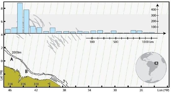
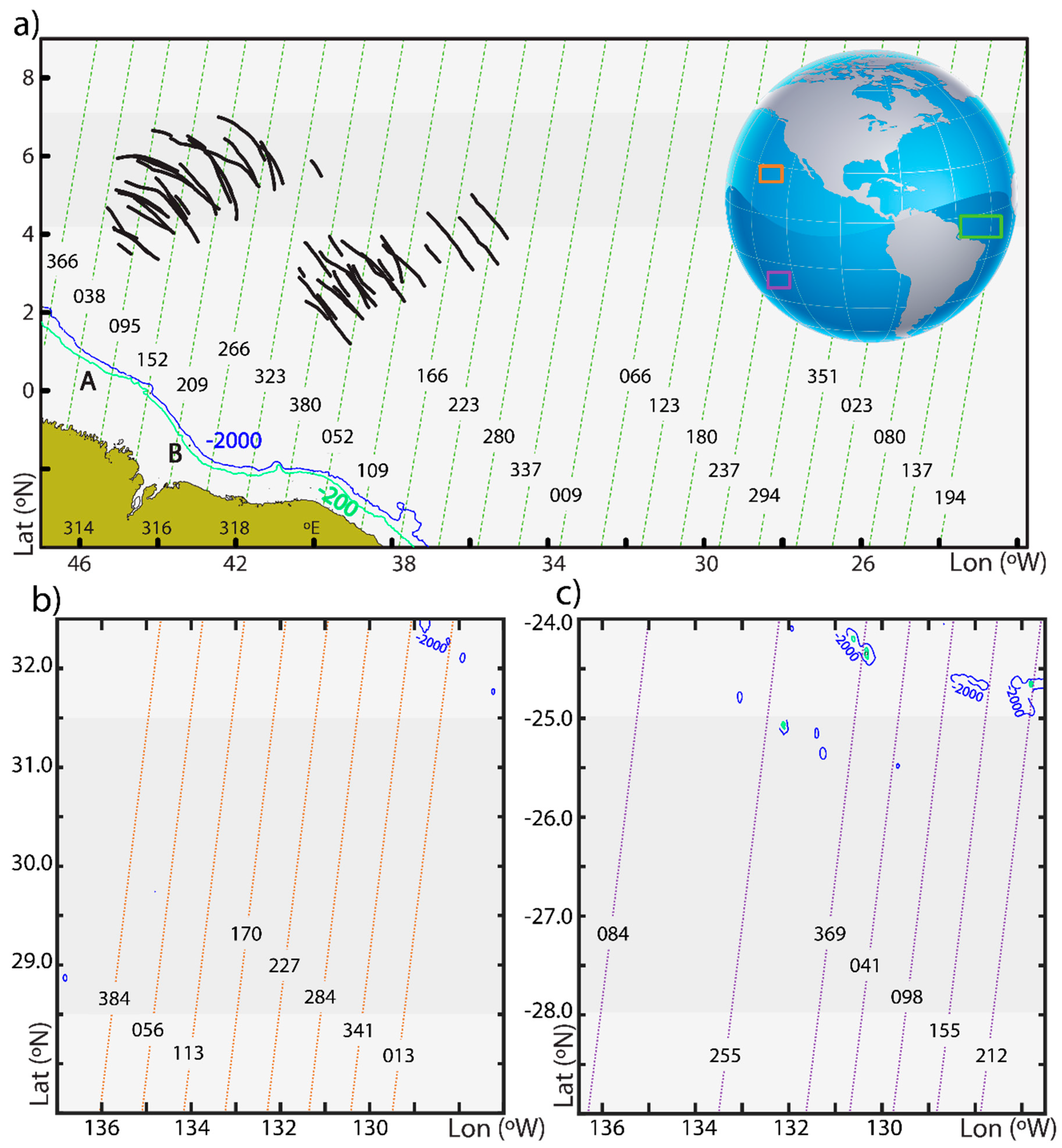
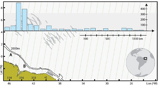
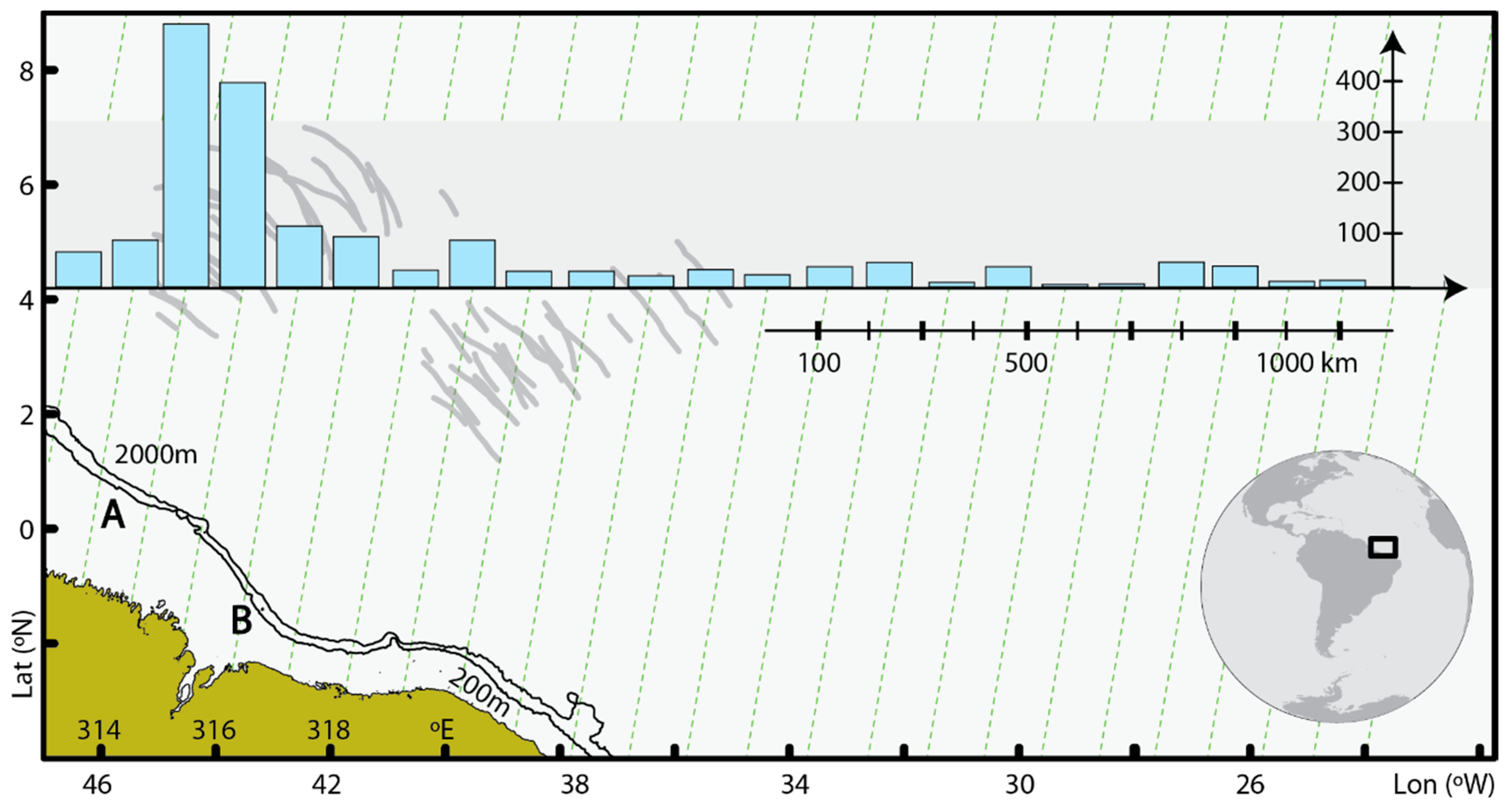
In order to test the algorithm, a region off the Amazon shelf was selected (see
Figure 1a), which is known for the existence of large amplitude ISWs propagating offshore for hundreds of kilometers, in deep water [
12]. There, internal wave amplitudes may exceed 100 m, wavelengths are typically 5 km, and crest lengths are about 150 km on average [
9]. The ISW crests studied in Reference [
9] with SAR images are represented in
Figure 1a in bold black, for reference. The region analyzed with the SRAL data, which range is 4.1–7.1 °N and spans from approximately 25°W to 46°W (more than 2000 km along the equator), is represented in gray shade in
Figure 1a. To the East of 35°W, no ISWs were detected with SAR images (see e.g., References [
9,
11]). This provides a framework for a validation exercise, since two different regions, one being an ISW hotspot and another practically void of ISWs are adjacent to each other along the equator, and both these regions can be readily examined for ISW detection with the algorithm presented in this paper. Note that the equator band is prone to severe weather, and hence the algorithm should cope to discriminate those weather related events from ISW surface roughness related events.
Furthermore, two other validation exercises were performed in remote regions of the Pacific Ocean (see
Figure 1b,c) where our best remote sensing knowledge indicates the absence of ISWs in SAR and sun glint images of appropriate spatial resolution. Those regions were defined based on our own search in available SAR image archives (Envisat and European Remote Sensing (ERS) missions) as well as the ISW map in Jackson et al. [
11]. In the case of the South Pacific, the geographic region is bounded in latitude by 25°S to 28°S, while in the case of the North Pacific, the region is bounded in latitude by 28.5°N to 31.5°N. Both those regions are bounded in longitude by approximately 127°W to 137°W (see
Figure 1).
In total we have analyzed 37 orbit cycles, corresponding to cycles 4–40 of Sentinel-3A. This sequence corresponds to a time span of more than 2 years. For reasons that will become apparent in
Section 3 and
Section 4, we fixed the along-track length scale to approximately 3° in latitude, corresponding to 1024 samples for each relative orbit. Altogether, we analyze 25 satellite altimeter tracks near the equator (off the Tropical Atlantic Ocean), 8 tracks for the North Pacific Ocean, and 7 tracks for the South Pacific Ocean.
3. Methods
Knowledge of the ocean surface slope distribution
S(
k) and the mean square slope (
) is essential to understanding the radar backscatter at normal incidence. The
is defined as,
where
S(
k) is the omnidirectional one-sided wave number slope spectrum and
k is the wave number [
13]. The
of waves in the wave number range that satisfies specular scattering conditions is inversely related to the normalized radar backscatter [
14,
15]. Assuming the surface wavefield as an isotropic Gaussian surface, as Cox and Munk [
1] did in their work of slope statistics, it is possible to apply the geometrical optics (GO) model [
16] of the integrated microwave backscatter cross section according to the expression
where
is an effective reflectivity,
is an effective mean square slope estimate, and θ is the pulse illumination incidence angle. Although Equation (2) neglects anisotropy of the ocean surface with respect to slope [
17] the isotropic form of the integrated cross section leads at most to an error of a few percent in the estimation of mean square slope [
15]. For satellite altimeter observations (near-nadir, i.e., θ = 0), Equation (2) reduces to give the mean square slope as
where the subscript
n is used to indicate nadir and
is understood to differ from a pure Fresnel reflectivity coefficient in that it may include diffraction effects (see e.g., References [
3,
18,
19]). The effective reflectivity coefficient
can be calibrated with field measurements of mean square slope [
3].
The effective mean square slope variable
given by Equation (3) can be evaluated from either
or
, but differs from the total mean square slope as measured by optical methods (e.g., Reference [
1]) in that it represents an integration of the wave number slope spectrum Equation (1) only up to a cutoff wavenumber corresponding to C-band and Ku-band radar wavelengths, respectively. Hence, these mean square slopes include contributions from all wave facets with dimensions greater than a cutoff wavelength λ
cutoff ≈ 3λ
i where λ
i is the radar wavelength [
14,
20]. For the Sentinel-3A Ku-band (λ
i = 2.1 cm) and C-band (λ
i = 5.5 cm) altimeters, these cutoff wavelengths are roughly 6.3 cm and 16.5 cm, respectively, which allows isolation of the mean square slope contribution of the small-scale waves between 6.3 cm and 16.5 cm by differencing the estimates from the two frequency bands.
Since footprint sizes for both Ku-band and C-band altimeter frequencies are the same for the Sentinel-3A (see e.g., Reference [
21]), meaning that the areas sampled by the two radar pulses are identical, the differenced mean square slope eliminates backscatter contributions from the longer waves. This methodology, proposed in Reference [
18] and applied in Reference [
3] to estimate global air–sea gas transfer velocity, is here introduced as a proxy to estimate the differenced mean square slope and detect short-period internal waves. It relies on the fact that short-period internal waves strongly modulate the surface wave spectrum in this short-wavelength range for various reasons. Amongst these reasons are the direct interaction between varying IW currents and wind-generated gravity-capillary waves [
19], modulations produced by variations of surface film concentration [
22], relative wind speed variability with respect to IW surface currents [
23], and specular reflection from breaking surface waves and small-scale surface waves generated by wave breaking [
24].
The differenced mean square slope
is defined as
that corresponds to the mean square slope over the approximate wave number range 40 ≤
k ≤ 100 rad/m. Accurate knowledge of the values of the parameters of
,
, and
is essential for evaluation of Equation (4). In order to obtain estimates for the above parameters, the authors in Reference [
3] calibrated their values against field measurements of mean square slope using a nonlinear, goal attainment, optimization technique. There are other values for these parameters in the literature, but Reference [
3] concluded that optimum values of
,
and
are 0.427, 0.617, and 3.61, respectively, in the framework of synergy with TOPEX altimeter data. In this study, we used the same parameters as Reference [
3], which were validated for wind speeds between 3 m/s and 9 m/s. Furthermore, a bias parameter γ is introduced to account for the
difference between TOPEX and Sentinel-3A radar altimeters (see Reference [
18]; and their Figure 3 there). The value of γ = 3.8 dB is determined by using a large amount of data, which means we need to add to the original Sentinel-3A
backscatter values the constant γ (in dB), in order to be able to use the same parameters as in Reference [
3]. We are then able to calculate the differenced mean square slope as defined in Equation (4).
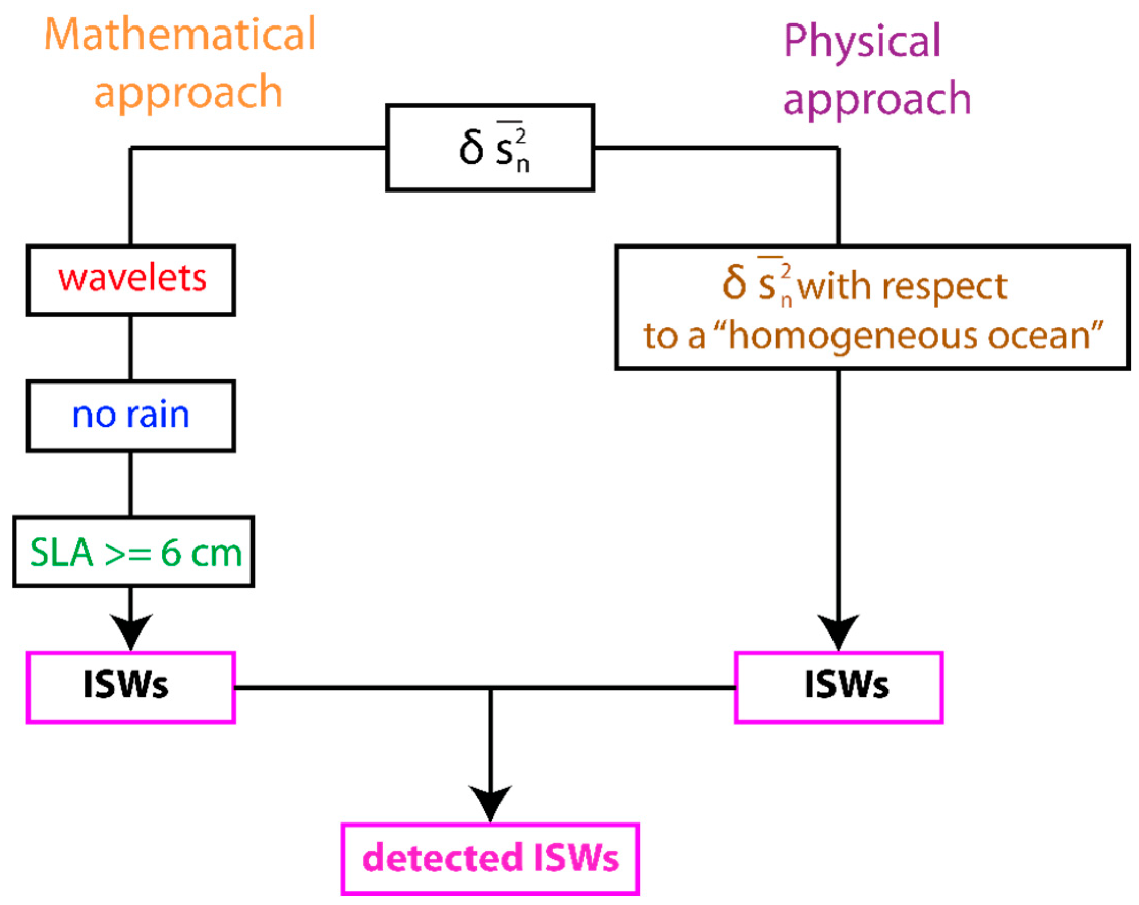
The obtained
from Equation (4) is then used in a wavelet analysis to search for adequate scales and patterns consistent with our expectation of ISW signatures in altimeter radar data (see schematics in
Figure 2, left side of flow diagram). Although the well-known Daubechies wavelets (of order 4, i.e., db4) have been used by the authors in Reference [
25] for identifying trains of solitons in SAR image profiles, here we choose the Haar wavelet (equivalent to Daubechies of order 1, i.e., db1) due to the solitary character of the internal waves in the study region. It proved to be the most successful wavelet in detecting solitons off the Amazon shelf, after rigorous comparison with OLCI cloud-free images of ISWs in the region. In particular, we use the stationary wavelet transform (SWT) and the signals provided in the details (i.e., the low-scale high-frequency components) of level 4, for searching the locations with largest variations in the signal. We define a threshold coefficient of 0.005 above which events in the
record calculated from Equation (4) are classified as potential signatures of ISWs.
After searching for potential ISW events in the
records as described above, we need to eliminate high-frequency events potentially affected by atmospheric features such as strong rainstorms. This is a severe problem in the study region, and along the equatorial zonal band in general, as it may produce alterations of radar backscatter (and hence
anomalies) that may be erroneously interpreted as ISWs by any automatic algorithm designed for detecting ISWs. Radar altimeter signals are attenuated by raindrops due to both absorption and scattering. The effects of rain contamination are often apparent from the erratic (high-frequency) variation of
, as well as significant wave height (see Reference [
26]). Since rain attenuation at the Ku-band is on an order of magnitude larger than that at the C-band, rain-contaminated observations from the Jason-2/3 dual-frequency altimeter are usually identified as an abrupt decrease in the
ratio between the Ku-band and C-band. However, in this study, we could not rely on this criterion to discard rain-affected measurements as those differenced dual-frequency
(high-frequency) fluctuations could also be due to IW surface manifestations (see also Reference [
8]). At present, our method to deal with rain-affected measurements consists of a threshold in the integrated columnar liquid water content
, here chosen as 0.1 kg/m
2, and water vapor content (
wv), whose limit was chosen as 60 kg/m
2 [
26] (as measured by the MWR on board Sentinel-3A). All radiometer measurements not satisfying
< 0.1 kg/m
2 or
wv < 60 kg/m
2 were discarded as probably being rain-affected.
Assuming that the SLA parameter available in current Level-2 data of the Sentinel-3A altimeter is physically meaningful, i.e., it provides a realistic measure of vertical displacements at the sea surface at those internal wave short-scales (of the order of hundreds of meters to a few kilometers along-track), it provides an additional criterion for detecting large amplitude ISWs as these have associated surface vertical displacements of the order of a few to tens of centimeters (see Reference [
27]). For the following step (see
Figure 2), the algorithm comprises a high-pass filtering of the original 20 Hz along-track SLA record by subtraction of a smoothed record (boxcar averaging) in scales of 30 km. This provides a high-frequency record whose average is zero in scales of 30 km, hence eliminating unwanted anomalies from larger scale (mesoscale) processes, and enhancing ISW scales. Events are “labelled” ISW-like events if, and only if, the filtered high-frequency SLA record exceeds 6 cm. It should be noted that ISWs in deep water, such as those in the study region, are waves of depression. This implies the associated surface elevations must be positive for mode-1 ISWs [
28], which are the most common internal waves in the ocean. Hence, one of the criteria used to detect a possible ISW-like event is
. It is based on hydrostatic approximation and a two-layer model (see Reference [
27]), in which the upper layer thickness is less than the lower layer (two-layer thicknesses and densities are determined by local parameters of stratification, i.e., a typical climatological buoyancy frequency profile whose depth of thermocline is taken for the depth of its maximum value). According to this approximation, for the study region off the Amazon shelf break, a SLA ≥ 6 cm means that ISWs with amplitudes greater than 20 m should be detected with the SAR altimeter. Other surface phenomena, such as organic films without dynamic origin, are not expected to produce a significant positive SLA. Schematics of the proposed method are presented in
Figure 2, which also includes a physical approach described next.
An independent physical approach (or criterion) to assess the potential of a high-frequency feature to be an ISW event has been established (see schematics in
Figure 2, right side of flow diagram). This is based on the values of
at a given wind speed measured by the altimeter. It is well known that radar backscatter measurements from satellite nadir looking altimeters can be converted in near-surface wind speed with useful accuracy (see e.g., Reference [
2]). Previous studies have demonstrated that estimates of near-surface wind speed can be inferred to within an rms accuracy of approximately 2 m/s from altimeter measurements of the normalized radar cross section
of the sea surface [
29]. Here we consider
measurements outside the interval of one rms equivalent wind speeds (considered as ±2 m/s) to be potentially indicators of an ISW event. In other words, we seek for a fit of
as a function of wind speed for the radar altimeter on board Sentinel-3A in a similar fashion as Cox and Munk’s [
1] optical measurements of wind speed and
. The data set of altimeter radar backscatter used to construct such a relationship is from an ocean region outside the equatorial zonal band and considered sufficiently homogeneous to be representative of background ocean conditions unaffected by surface manifestations of high-frequency ocean dynamics (see details in the next Section). Once this “
versus wind speed” relationship is established (see next Section of the paper) we have a tool to assess reasonable bounds of
for a given near-surface wind speed. When a
measurement is outside the expected value for the measured wind speed in the vicinity of an ISW event, the position of such
measurement is considered affected by an ISW event (see
Section 4). The criterion for ISW detection is given by the following condition,
where
is the differenced mean square slope retrieved for Sentinel-3A defined in Equation (4) with the appropriate coefficients and
U10 is the altimeter wind speed at 10 m height above the sea level in neutral atmospheric conditions available in the Sentinel-3A Level 2 data (see Reference [
29] for details). Note that
U10 is provided in 1 Hz, and it was interpolated to 20 Hz before use. This means that
U10 is approximately the average wind speed on spatial scales of 6 km.
All the above-mentioned conditions and constraints offer a reasonable basis for development of a method for automatic detection of ISWs in altimeters, such as those onboard Sentinel-3A and 3B.
4. Results
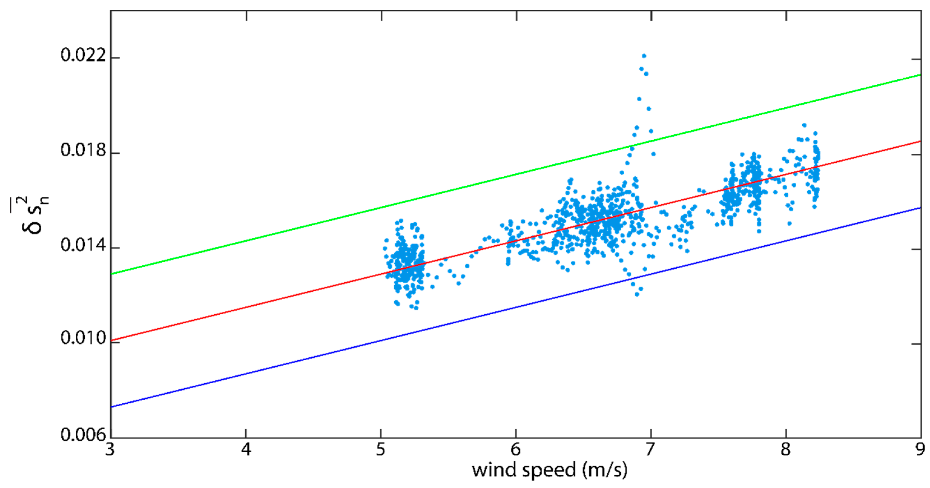
A linear fit established with the
versus
U10 altimeter data provides the basis of our physical approach described in
Section 3, and is given by
= 0.00149 ×
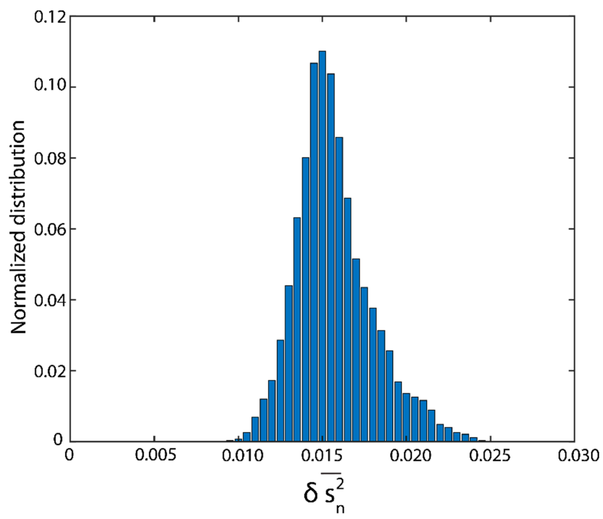
U10 + 0.00569. The linear fit is obtained for the region of the South Pacific Ocean defined in
Section 2, which is known to be void of high-frequency events such as ISWs or well-defined and sharp ocean fronts. The region is defined based on our previous knowledge of SAR image analysis (in archived data from the Envisat and ERS-1/2 missions). The geographic coordinates of the region comprises an area between 25–28°S and 127–137°W (see also
Section 2 and
Figure 1c). Sentinel-3A SRAL data of relative orbits 041, 084, and 098 from cycles 013 through 030 were analyzed and the normalized distribution of the
is shown in
Figure 3. While the linear fit described above, and the distribution in
Figure 3, include satellite overpasses only from cycles 013 to 030 (because when the method was implemented there were no further cycles available), we reiterated the fitting analysis for the time of writing of this paper (i.e., from cycle 004 until cycle 040) and found no significant alteration in the fitting. The
distribution shown in
Figure 3 excludes rainstorm events and other high-frequency major atmospheric events as explained in
Section 3.
An example of the application of the method (physical approach) to a particular Sentinel-3A overpass in the tropical Atlantic off the Amazon shelf is presented in
Figure 4, where
calibrated data points outside the one rms equivalent
U10 wind speeds interval (considered as ±2 m/s) are indicative of possible ISW events. In
Figure 4, the red line corresponds to the linear fit described above and the blue and green parallel lines are displaced in the horizontal by ±2 m/s, respectively. The results of the “physical approach” described above are then compared with the “mathematical approach” based on wavelet analysis of the
signals.
Figure 5 and
Figure 6 present the results of the algorithm for relative orbit 152 of cycle 036, dated 27 September 2018 and for which the ISW detection is validated with an OLCI cloud-free image (shown in
Figure 7) that reveals clear evidence of a large amplitude ISW.
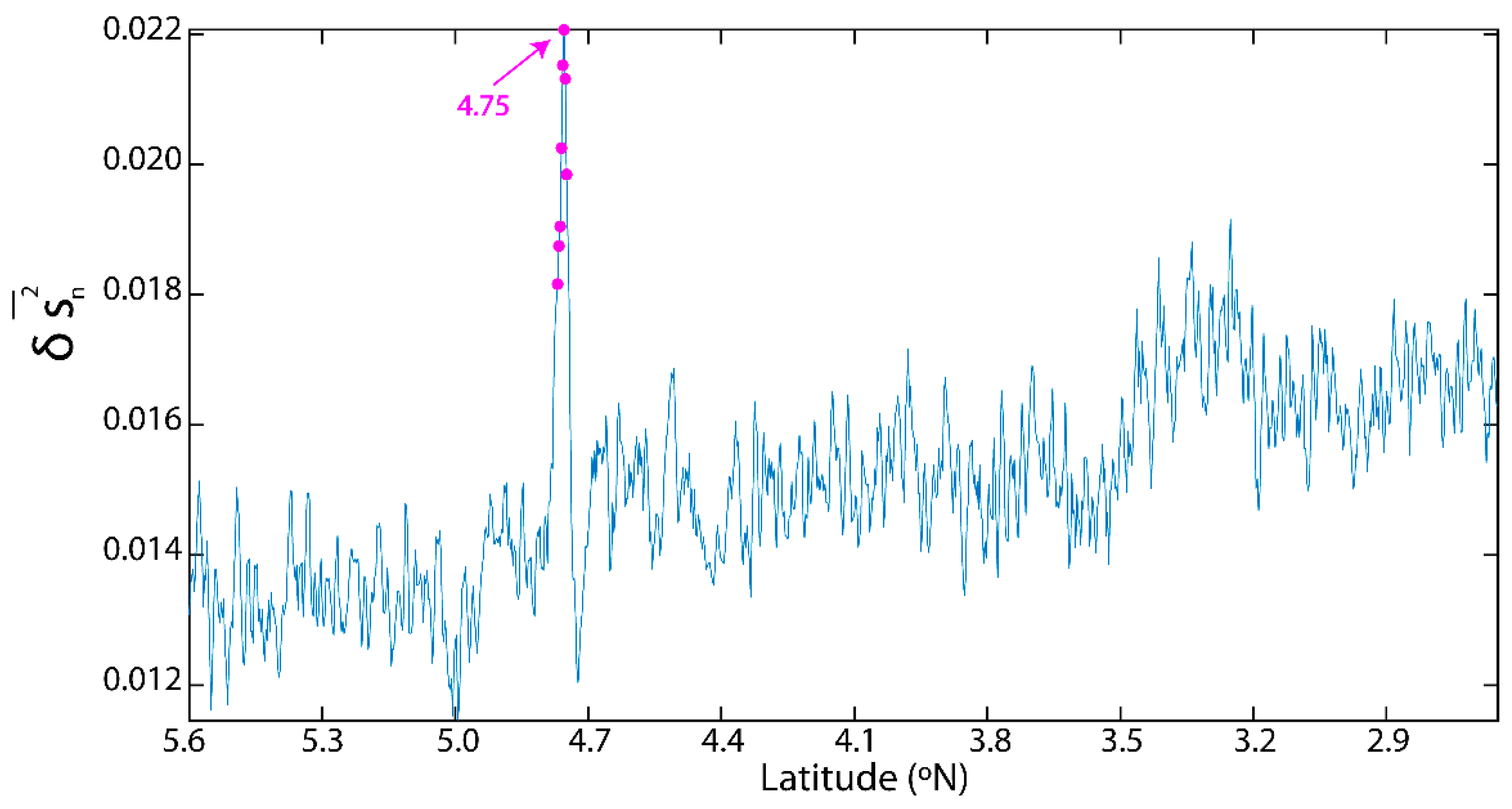
A large solitary wave is depicted in
Figure 6 for this same orbit (152 of cycle 036), the only feature detected by the algorithm in this paper within the stretch of approximately 300 km along-track from 2.6°N to 5.6°N. This particular orbit and cycle is chosen because it corresponds to a cloud-free OLCI image (shown in
Figure 7) that permits validation of the algorithm. Note that, in the study region, the earliest appearance of ISWs has been reported at approximately 4°N (see References [
9,
12]), hence the solitary wave detection at 4.8°N in the SRAL record is in accord with our expectations. In
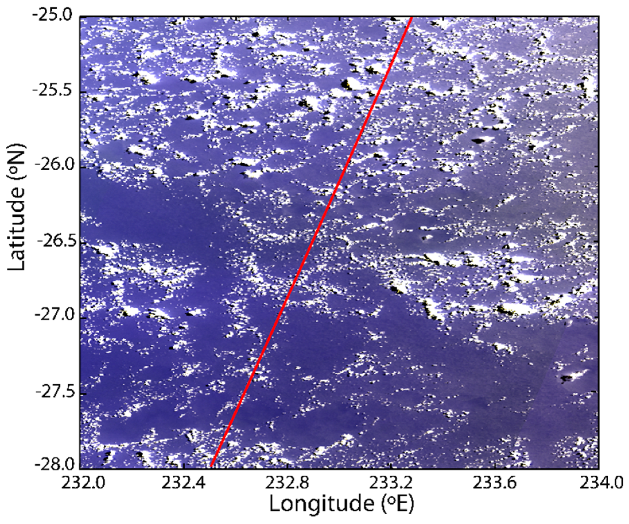
Figure 7, an extract of an OLCI quasitrue color Level 1b image is shown over the same stretch of ocean as the radar altimeter track of relative orbit 152 of cycle 036 that is shown in
Figure 6 (red line). It is confirmed that a single ISW is visible at approximately 4.75°N.
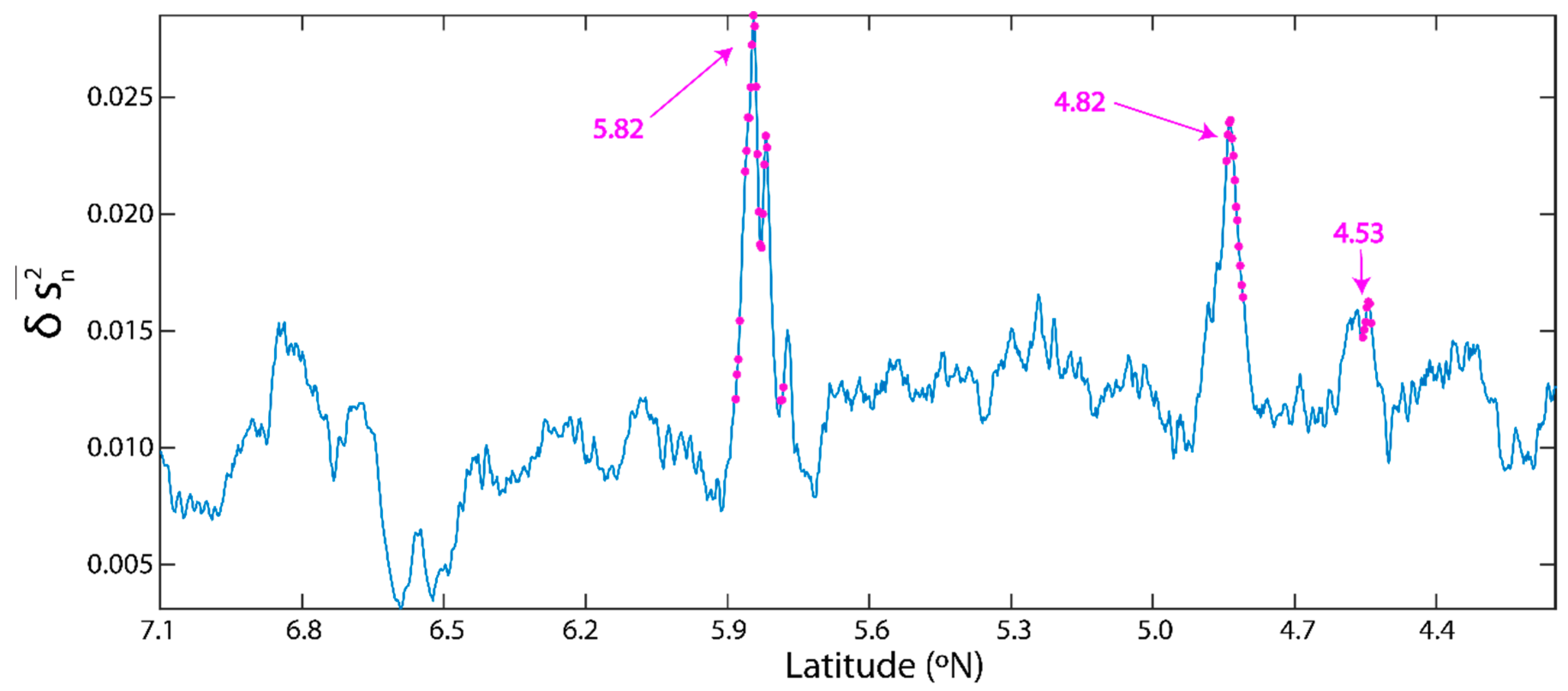
One more example of synergy in cloud-free conditions is provided (see
Figure 8 and
Figure 9 below), where ISWs are detected simultaneously in the SRAL and the OLCI over the same region. In
Figure 8, the final result of the detection algorithm is presented for relative orbit 095 of cycle 018, where several solitary waves are depicted within the along-track stretch from 4.1°N to 7.1°N. Waves are detected at 4.53°N, 4.82°N, and 5.82°N, all being confirmed by visual inspection in the cloud-free OLCI image shown in
Figure 9.
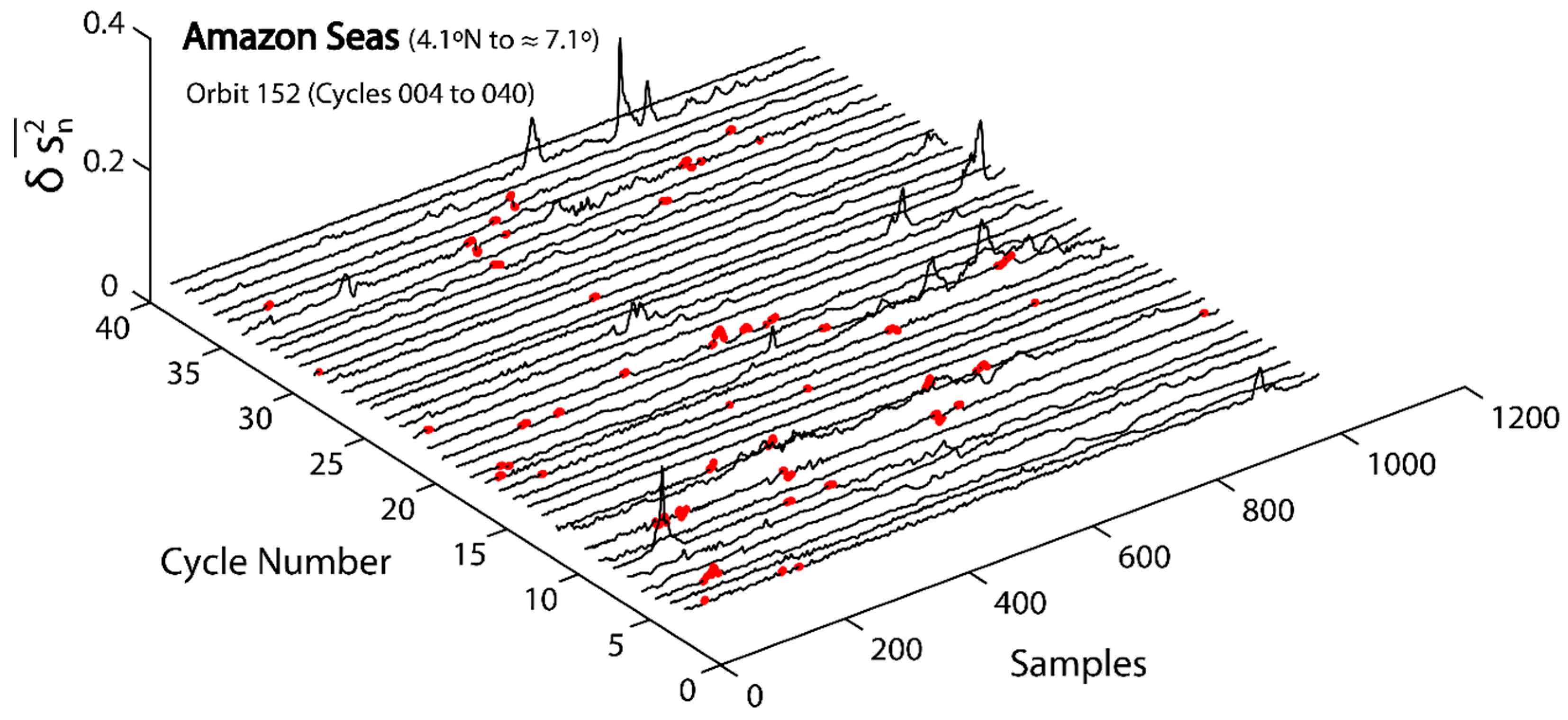
The wave propagation direction and their dimensions are thus optimal for observation with diurnal SRAL overpasses, resulting in positive detection by the algorithm most of the times, as it is shown in
Figure 10. Detections were identified along two major Sentinel-3A satellite tracks, namely relative orbits 095 and 152 (see below). In the case of relative orbit 152, and over the stretch of the deep tropical Atlantic Ocean under consideration, ISWs are detected in 18 out of 37 analyzed cycles (i.e., 49% of the time). The ISW observations were validated by visual inspection of OLCI cloud-free images of ISWs in 12 out of 18 cycles, where they were validated in 63% of the cases (even “cloud-free” images contained clouds that hampered 100% validation of the cases). All the other remaining 6 cycles correspond to cloud-covered conditions. All clear signatures of ISWs observed in the OLCI cloud-free images were detected in the SAR algorithm. In some instances, the SAR algorithm detected signatures in cloud-free conditions that were not apparent in the OLCI. We attribute those cases to insufficient sun glint in the OLCI to produce strong enough roughness signatures.
In the case of relative orbit 095, ISWs were detected in 19 out of 37 analyzed cycles (i.e., 51% of the time). The ISW observations were validated by visual inspection of OLCI cloud-free images of ISWs in 9 out of 19 cycles, where they were validated in 38% of the cases. Orbit 095 was generally more cloud contaminated than orbit 152. Hence we present in
Figure 10 the results of the SRAL detection algorithm for relative orbit 152, which is the altimetry track with the best rate of validation, corresponding to the latitude interval between 4.1°N and 7.1°N.
5. Discussion and Final Remarks
Ideally, the detection method should be validated with in situ measurements of ISWs simultaneous with the satellite overpasses at the same exact positions. Unfortunately, to the best of our knowledge, these are not available in the study region. In fact, we are unaware of any available in situ measurements of internal solitons coincident with the Sentinel-3 satellite tracks during the duration of its mission to-date. Hence, we rely on our ability to recognize ISWs in sun glint visible medium-resolution satellite imagery, from sensors such as OLCI and MODIS (see e.g., Reference [
11]).
The results of the automatic detection, shown in
Figure 10 for relative orbit 152, are qualitatively in accord with our expectations, since ISW-like events are encountered for 49% of the overpasses and it is known that ISWs in the study region are regularly observed in all seasons and are independent of the spring-neap tidal cycles [
9]. Altogether, the algorithm was tested for 25 Sentinel-3A relative orbits, aligned in spatial sequence along the zonal direction in the equator band approximately limited in latitude within 4.1°N to 7.1°N (see
Figure 1a). Overpasses crossing the geographic region where ISWs are known to exist at those latitudes include, relative orbits 095, 152, 209, and 266. Another 19 relative orbits to the east of relative orbit 266 were also tested using the algorithm. Scrutiny indicates a significantly higher detection rate of ISW-like events for the satellite tracks crossing the ISW hot spot zone identified in
Figure 1a, which is based in the study of Magalhaes et al. [
9] who used Envisat and ERS images. In
Figure 11 we present a bar diagram with the number of SRAL cells detected as ISW-like events with the algorithm in this paper. According to our estimates, the average number of detections of ISW-like events is almost nine-fold higher in the hot spot zone of Magalhaes et al. [
9] (relative orbits 095, 152, 209, and 266) as compared to the average number of positive detections in the other tracks to the east, along the equator (see also
Table 1 for details).
The average number of detections of ISW-like events in the study regions defined in
Section 2 in 37 orbit cycles (since cycle 004 to 040) are shown in
Table 1.
In the case of the North Pacific Ocean, whose exact region of interest is identified in
Section 2 (
Figure 1b), the average number of ISW-like event detections is 17, which is about seventeen times smaller than in the ISW hot spot in the tropical Atlantic Ocean. In the South Pacific Ocean, whose region of interest is identified in
Section 2 (
Figure 1c), the average detection number of ISW-like events is of just 13 cases for the 37 orbit cycles in question, hence being 22 times less than the average number of detection in the ISW hot spot zone. In both these Pacific Ocean regions devoid of ISWs, the average number of positive detections is significantly lower than the average detection rate off the Amazon shelf where we know the presence of large amplitude ISWs. We feel that this rate of detection favors the algorithm presented here, providing an estimate figure of only about 5% of false detections.
Nevertheless, it is natural to question why the number of detected ISW-like events is not zero in the regions devoid of large amplitude ISWs. There are several reasons that might explain this fact: (1) Other high-frequency phenomena such as ocean fronts, film slicks, oil spills, ship wakes, etc.; (2) tropospheric downbursts and microbursts may alter the sea surface roughness in spatial scales similar to ISWs that are not recognized by our present liquid water and water vapor discarding criteria; (3) other spurious data resulting from various ocean and atmospheric effects or even anthropogenic effects. It is well known that those small-scale processes or events produce a signature in SAR images of the ocean surface (e.g., References [
30,
31].) Hence, it is reasonable to assume that some of those high-frequency phenomena at the sea surface interface produce also strong signatures in the
field of SAR altimetry data, which are readily depicted by the algorithm in this paper. Hence, we interpret the ISW-like event detection outside the zones of ISWs as possibly resulting from multiple other small-scale processes. It is then reasonable to assume that some of the ISW-like detections in the Amazon region are also due to other high-frequency phenomena, and not ISWs. At the moment the algorithm is not capable of dealing with such false alarms.
On some occasions, we noted that the detection of ISW-like events coincided with convection cells and vertically developed clouds, which were not flagged out by the liquid water and water vapor thresholds used here. In such cases, it is then likely that the high-frequency signatures classified as ISW-like events result from subcell resolution artifacts of the microwave radiometer used to measure the liquid and water vapor contents. In the future, we plan to look at this issue in order to improve the detection algorithm, but it is likely that a fully automated algorithm to detect ISWs would then require use of synergy images (OLCI and the thermal infrared SLSTR—sea and land surface temperature radiometer) to discard such cases of severe atmospheric effects at microwave radiometer subcell resolutions.
To further illustrate the capabilities of the algorithm developed here, we next show two examples of when the absence of ISWs is confirmed both in the OLCI cloud-free images and the SRAL record.
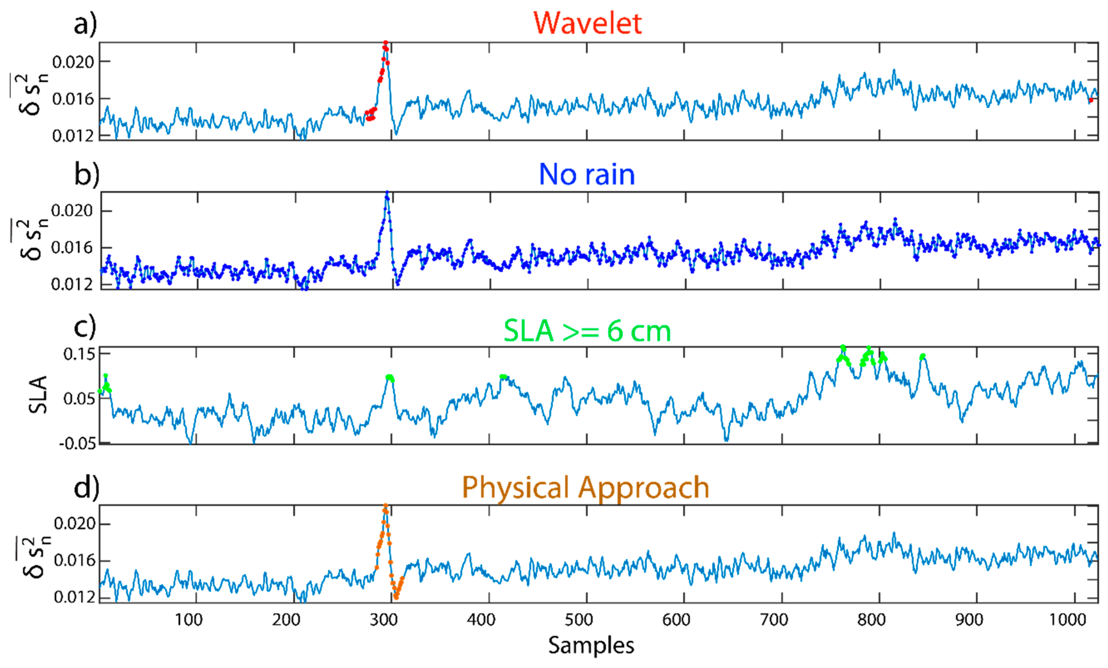
Figure 12 shows an OLCI quasitrue color image of the study region in the North Pacific Ocean (defined in
Figure 1b). In practice, this is a cloud-free OLCI image where the satellite track (relative orbit 170, cycle 033) crosses a large area of sun glint. Scrutiny of this, and other images of its kind, reveal small roughness variations along-track which are incapable to be detected in the algorithm (see
Figure 13). Only a few SLA along-track variations exceed the threshold used in the algorithm (6 cm) to detect possible ISW-like events (
Figure 13c), but those are not matched by the wavelet criteria (
Figure 13a), neither by the physical approach threshold used to analyze the
(
Figure 13d). Hence, the algorithm fails to detect possible ISW-like events, which is confirmed by visual inspection of
Figure 12. In
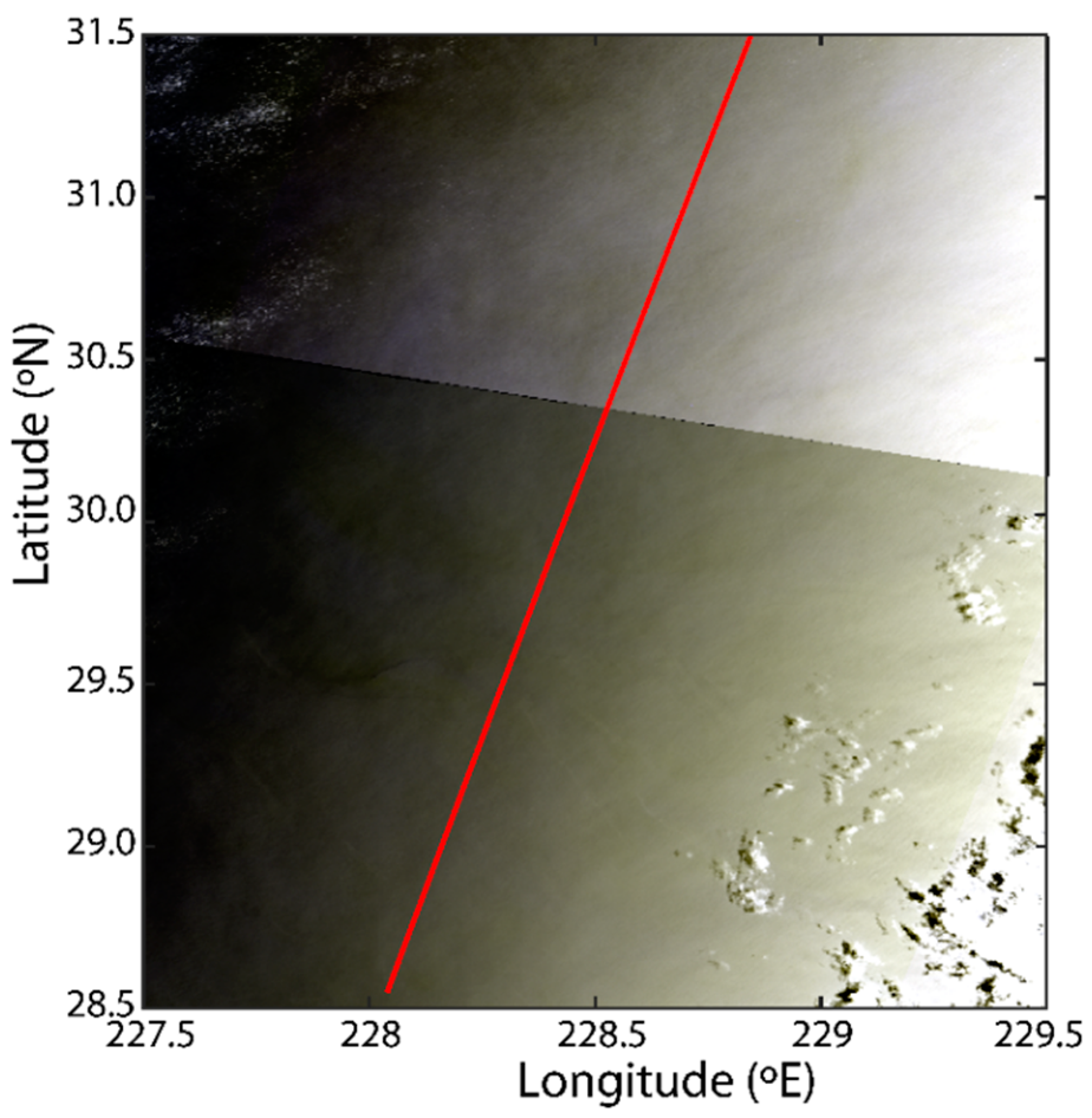
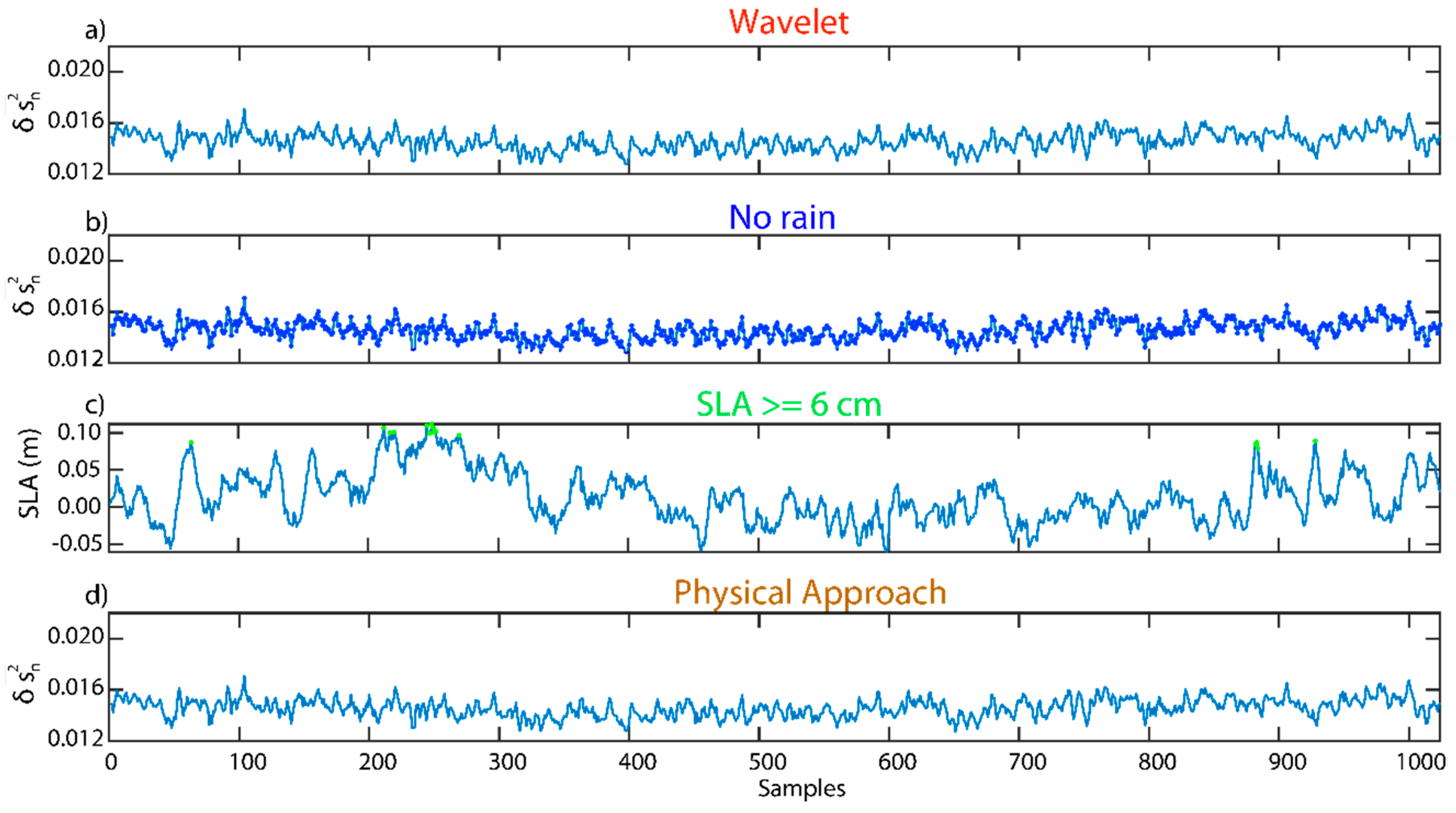
Figure 14 a similar situation is shown for the study region in the South Pacific Ocean.
Figure 14 shows an OLCI quasitrue color image of the study region in the South Pacific Ocean (defined in
Figure 1c). Here too, a relatively cloud-free OLCI image is shown along the satellite track (that of relative orbit 098, cycle 029). No significant roughness variations along-track can be observed, which is further confirmed in the along-track records in
Figure 15a. As in the case of
Figure 13c (North Pacific), only a few SLA along-track variations exceed the threshold used in the algorithm (6 cm) to detect possible ISW-like events, but those are not matched by the wavelet criteria (
Figure 15a), neither by the physical approach threshold used to analyze the
(
Figure 15d).
In summary, we have shown that the SAR mode altimeter on board Sentinel-3 is sensitive to surface roughness manifestations originating from large-amplitude ISWs in the tropical ocean. A methodology was developed for the automatic detection of ISW-like events based on satellite estimation of mean square slopes along-track. The mean square slope estimates were based on the dual-frequency capabilities of Sentinel-3A radar altimeter, and benefit from the SAR-enhanced spatial resolution along-track (300 m). The results of the method were partially validated with sun glint OLCI cloud-free images, acquired simultaneous with the SAR altimeter, a synergy capability that is only available for Sentinel-3A and 3B. The results suggest that SRAL-enhanced Level-2 altimetry data, or other advanced processing scheme such as the fully focused SAR [
32], may be used on a routine basis to detect large-amplitude internal solitary waves over the tropical ocean and marginal seas. The algorithm presented in this paper is expected valid for wind speeds between 3 m/s and 9 m/s.


