Author Contributions
Conceptualization, R.W., H.L., and Z.F.; methodology, R.W.; software, R.W.; validation, H.L. and Z.L.; formal analysis, Q.W.; investigation, Z.L. and H.L.; resources, H.L.; data curation, Z.L., R.W., and Q.W.; writing—original draft preparation, R.W.; writing—review and editing, R.W., H.L., and Q.W.; visualization, R.W. and Z.L.; supervision, H.L. and W.S.; project administration, H.L.; funding acquisition, H.L. and F.Z.
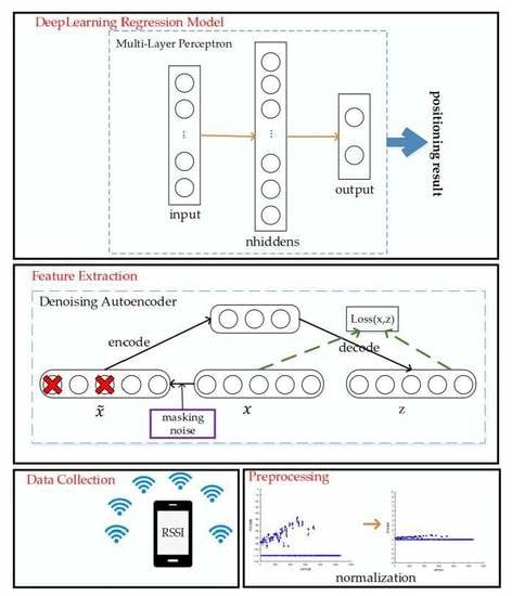
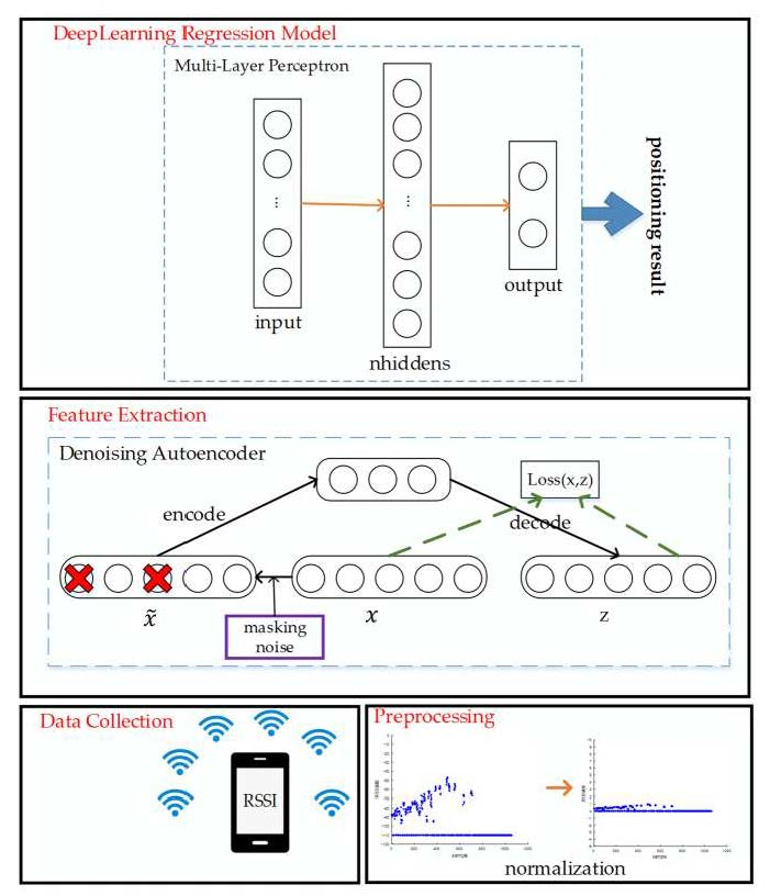
Figure 1.
Overall structure of our proposed positioning algorithm.
Figure 1.
Overall structure of our proposed positioning algorithm.
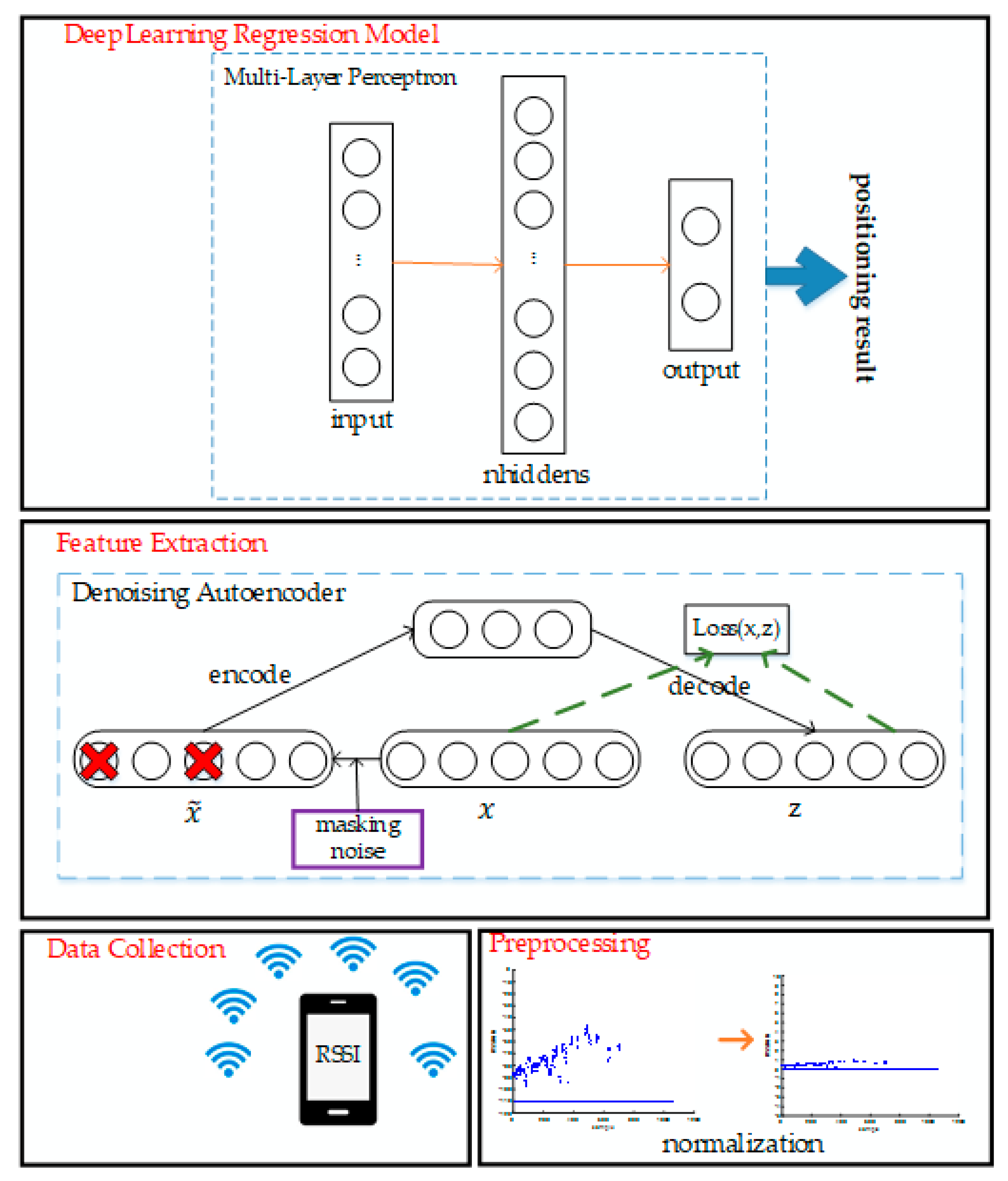
Figure 2.
The dynamic fluctuation of Wi-Fi signal with time in a teaching building. (a) RSSI data distribution of different Wi-Fi signals at different times in a specific location. (b) RSSI changes of different Wi-Fi signals over a 10-day period in a specific location.
Figure 2.
The dynamic fluctuation of Wi-Fi signal with time in a teaching building. (a) RSSI data distribution of different Wi-Fi signals at different times in a specific location. (b) RSSI changes of different Wi-Fi signals over a 10-day period in a specific location.
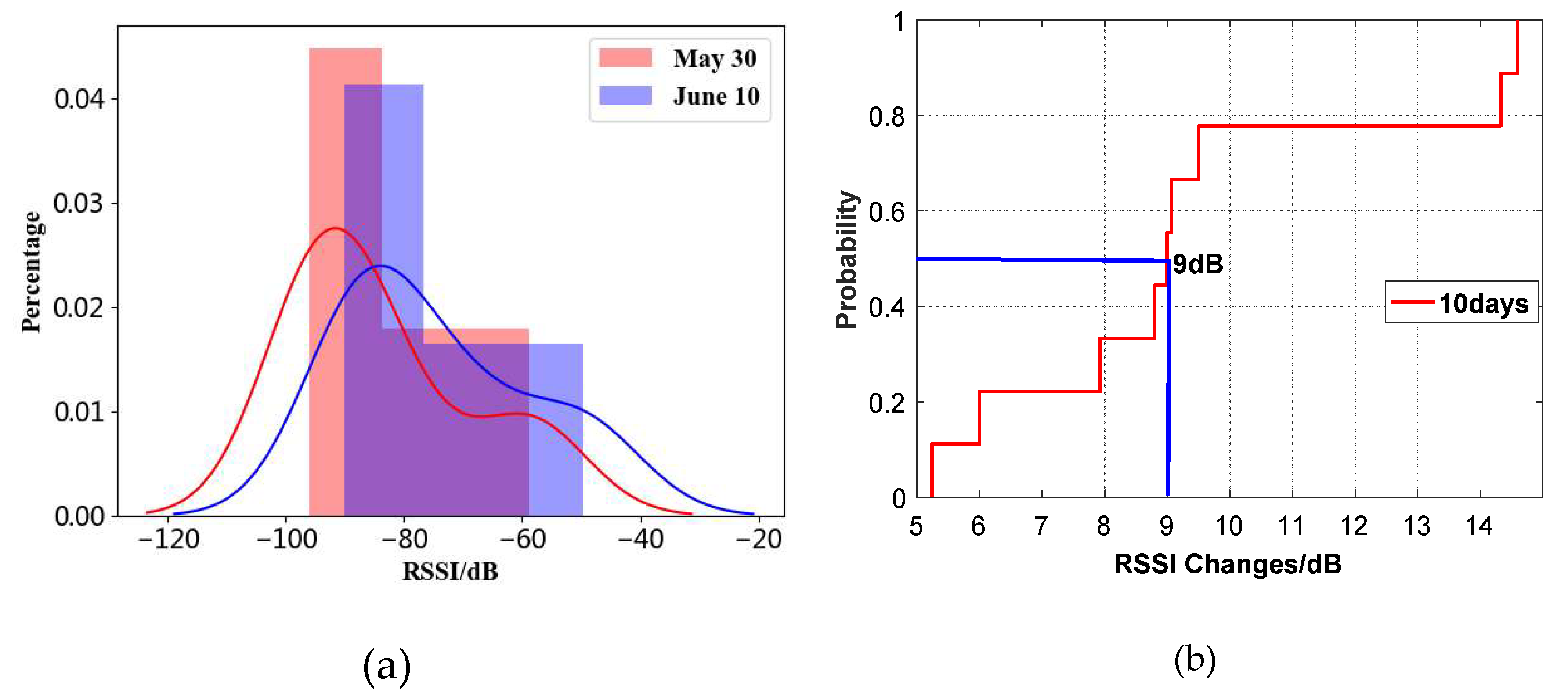
Figure 3.
The dynamic fluctuation of Wi-Fi signal with time in an office building. (a) RSSI data distribution of different Wi-Fi signals at different times in a specific location. (b) RSSI changes of different Wi-Fi signals over a 50-day period in a specific location.
Figure 3.
The dynamic fluctuation of Wi-Fi signal with time in an office building. (a) RSSI data distribution of different Wi-Fi signals at different times in a specific location. (b) RSSI changes of different Wi-Fi signals over a 50-day period in a specific location.
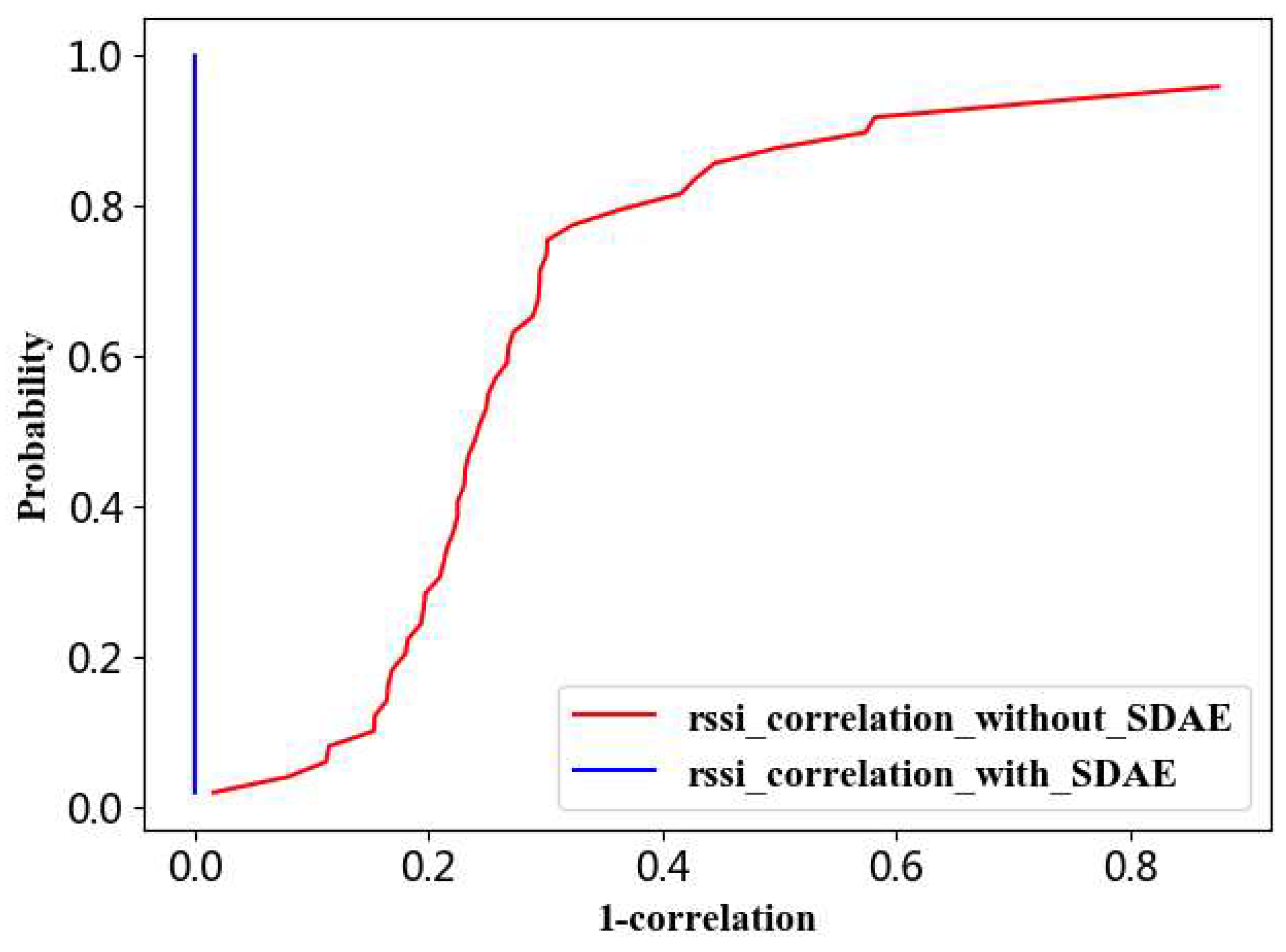
Figure 4.
Correlation of RSSI samples of the original Wi-Fi data and the new-collected Wi-Fi data at the same position before SDAE and after SDAE.
Figure 4.
Correlation of RSSI samples of the original Wi-Fi data and the new-collected Wi-Fi data at the same position before SDAE and after SDAE.
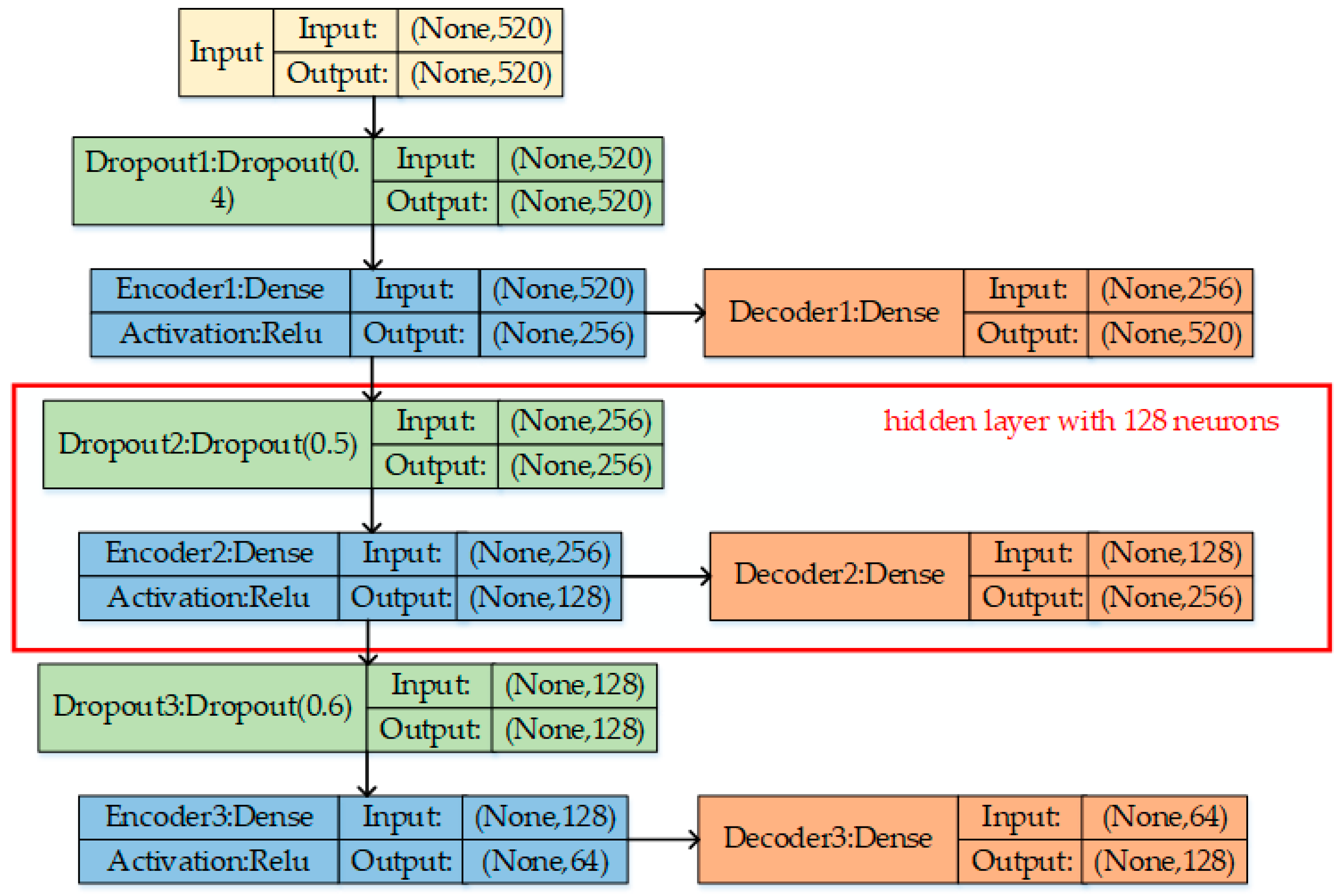
Figure 5.
The SDAE network structure.
Figure 5.
The SDAE network structure.
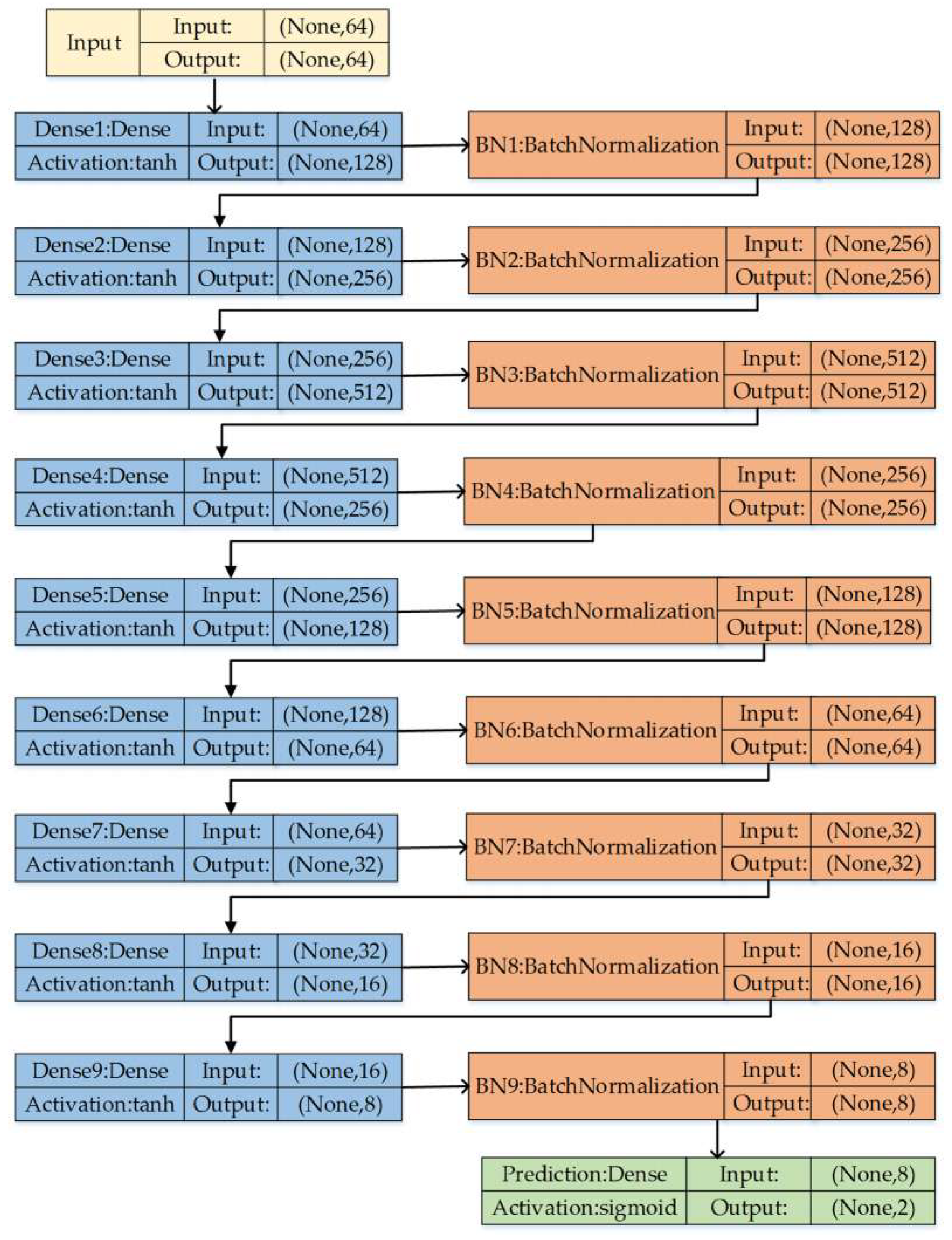
Figure 6.
Regression model network structure based on MLP.
Figure 6.
Regression model network structure based on MLP.
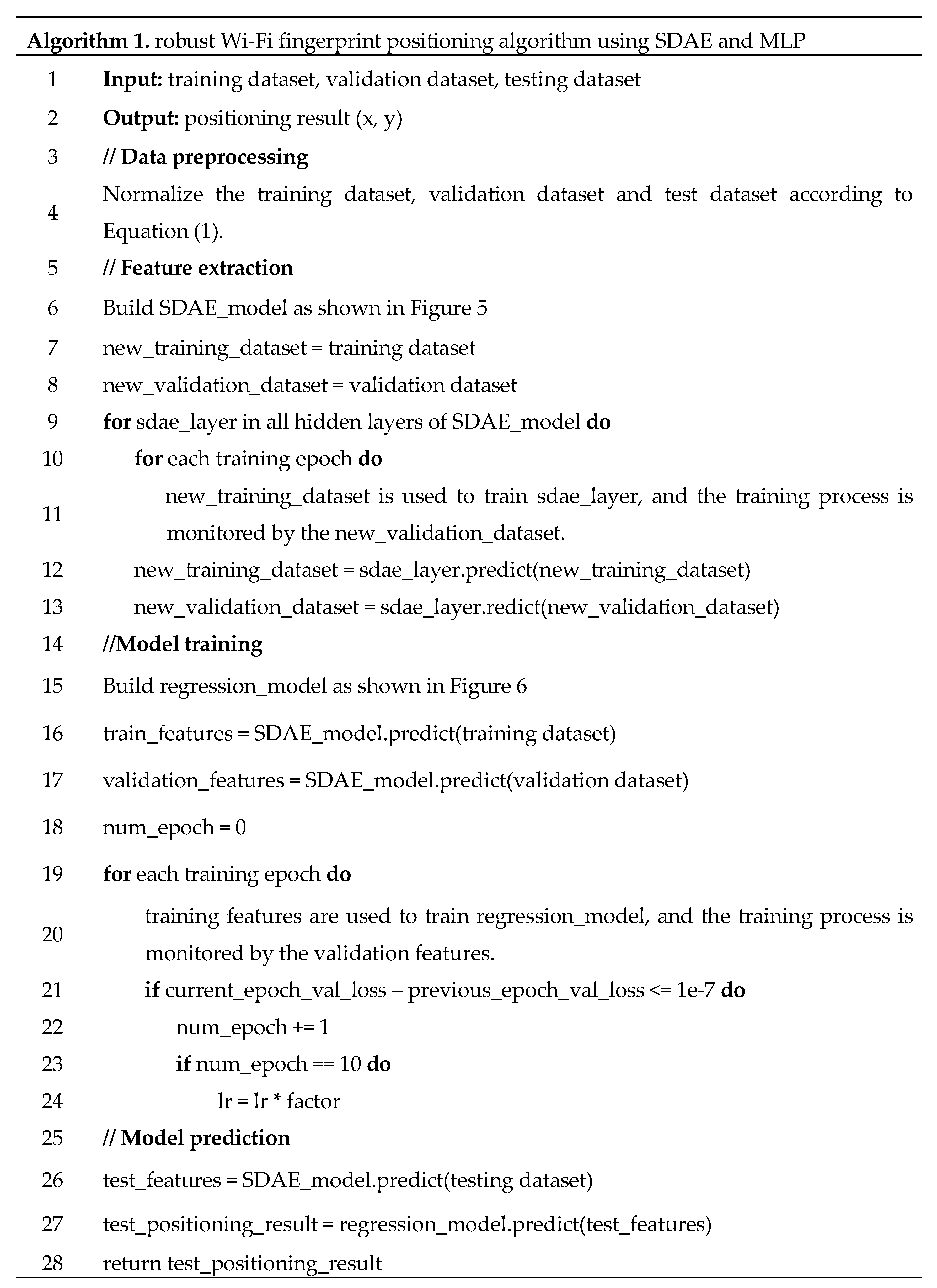
Figure 7.
The pseudo code of the robust Wi-Fi fingerprint positioning algorithm using SDAE and MLP.
Figure 7.
The pseudo code of the robust Wi-Fi fingerprint positioning algorithm using SDAE and MLP.
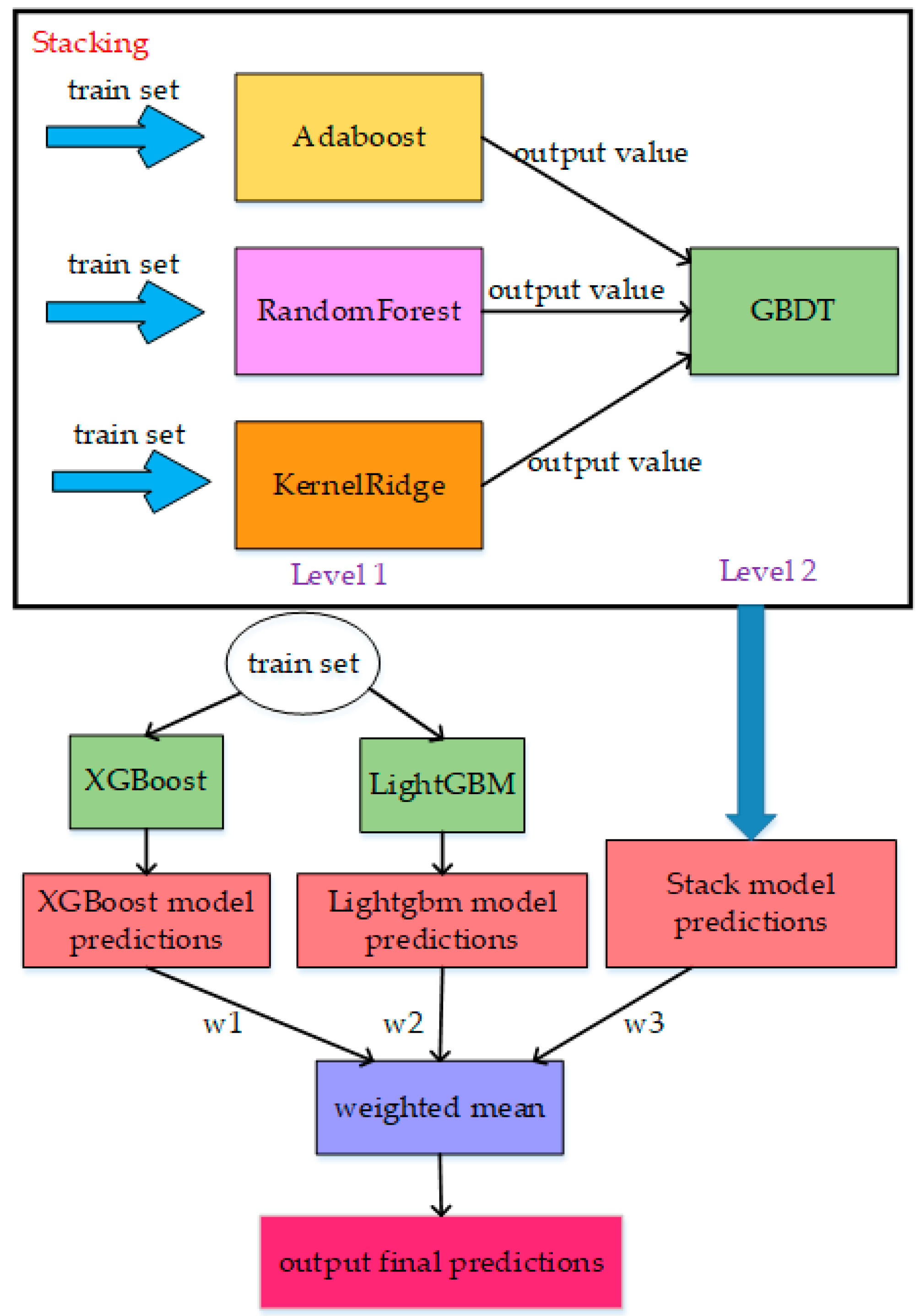
Figure 8.
The overall framework of the tree-fusion-based regression model.
Figure 8.
The overall framework of the tree-fusion-based regression model.
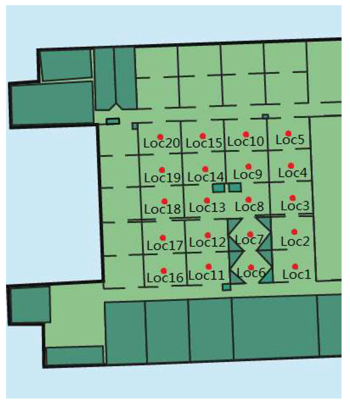
Figure 9.
The sampling positions of Dataset2 in our laboratory.
Figure 9.
The sampling positions of Dataset2 in our laboratory.
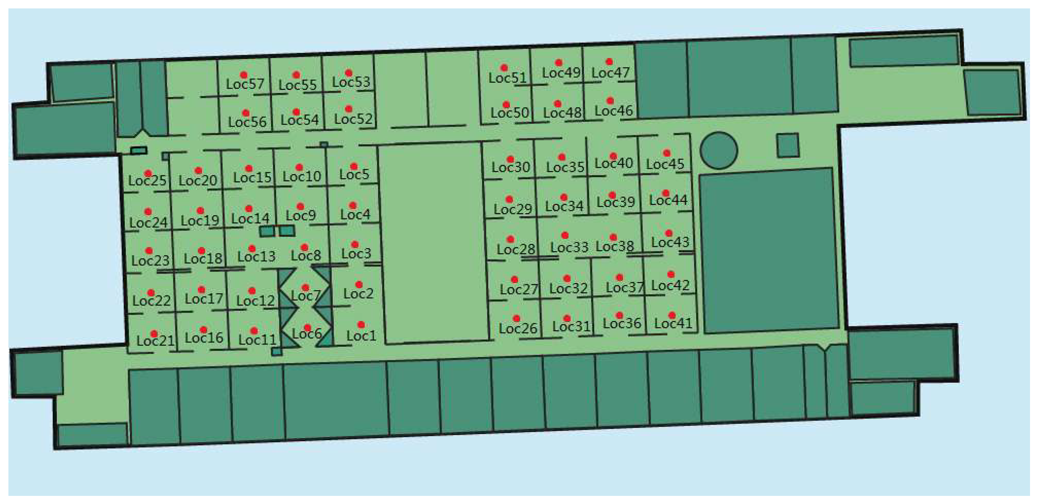
Figure 10.
The sample position of the Dataset3 in our laboratory.
Figure 10.
The sample position of the Dataset3 in our laboratory.
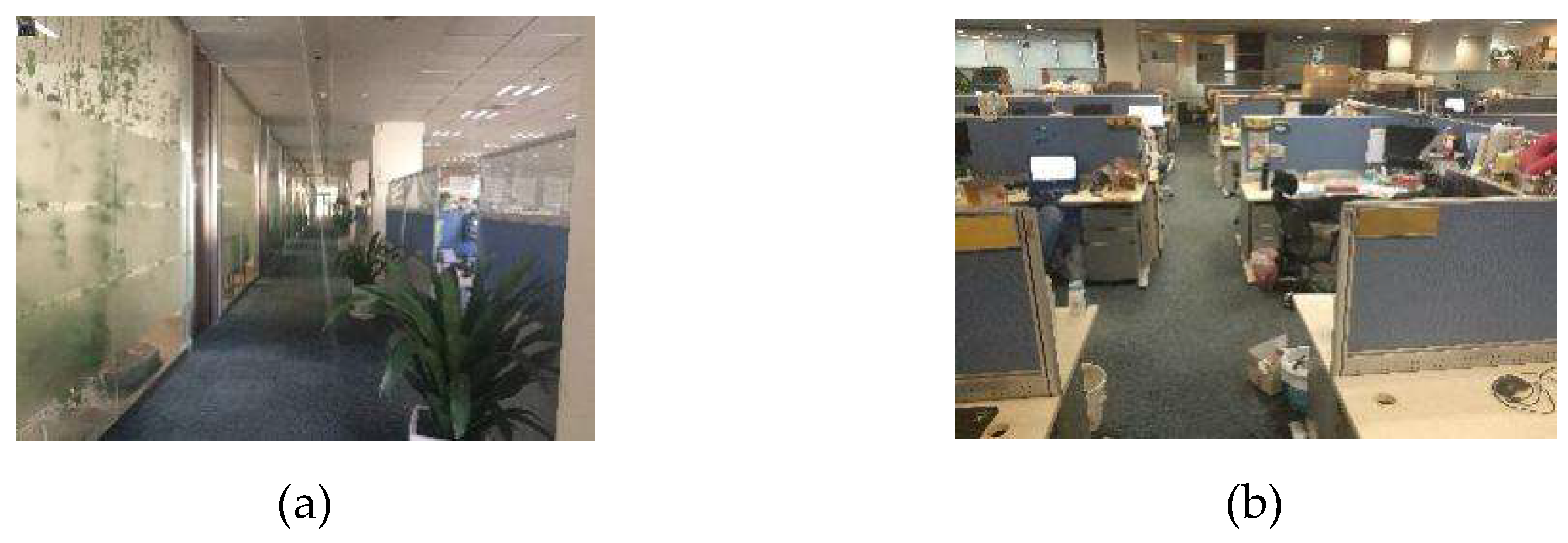
Figure 11.
The experimental environment: (a) corridor; (b) work-station.
Figure 11.
The experimental environment: (a) corridor; (b) work-station.
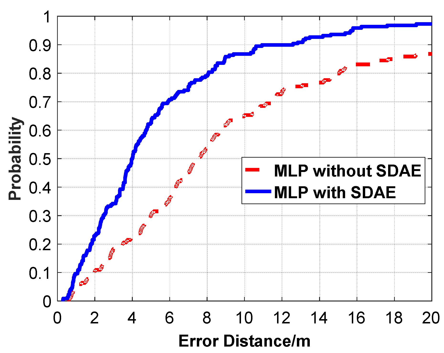
Figure 12.
Comparison of CDF (Cumulative Distribution Function) positioning errors between the algorithm with feature extraction and the algorithm without feature extraction.
Figure 12.
Comparison of CDF (Cumulative Distribution Function) positioning errors between the algorithm with feature extraction and the algorithm without feature extraction.
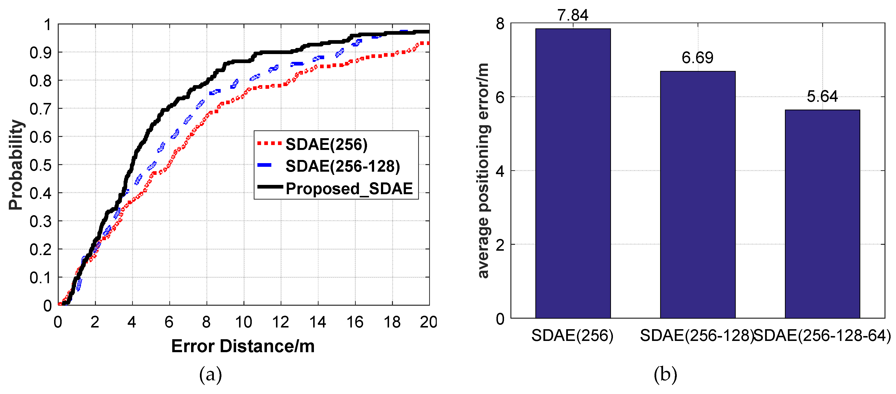
Figure 13.
The positioning accuracy using different SDAE network structures. (a) CDF positioning errors. (b) Average positioning errors.
Figure 13.
The positioning accuracy using different SDAE network structures. (a) CDF positioning errors. (b) Average positioning errors.
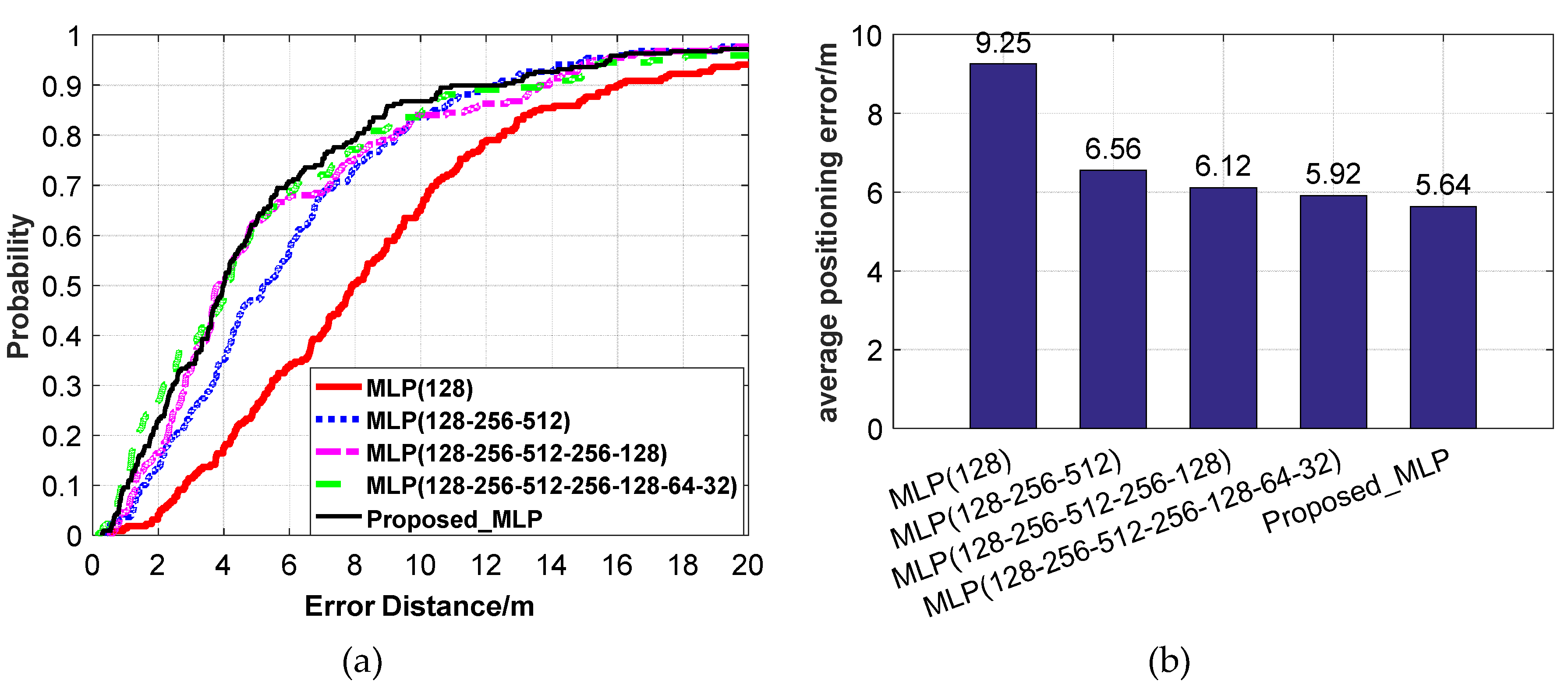
Figure 14.
The positioning accuracy using different MLP network structures. (a) CDF positioning errors. (b) Average positioning errors.
Figure 14.
The positioning accuracy using different MLP network structures. (a) CDF positioning errors. (b) Average positioning errors.
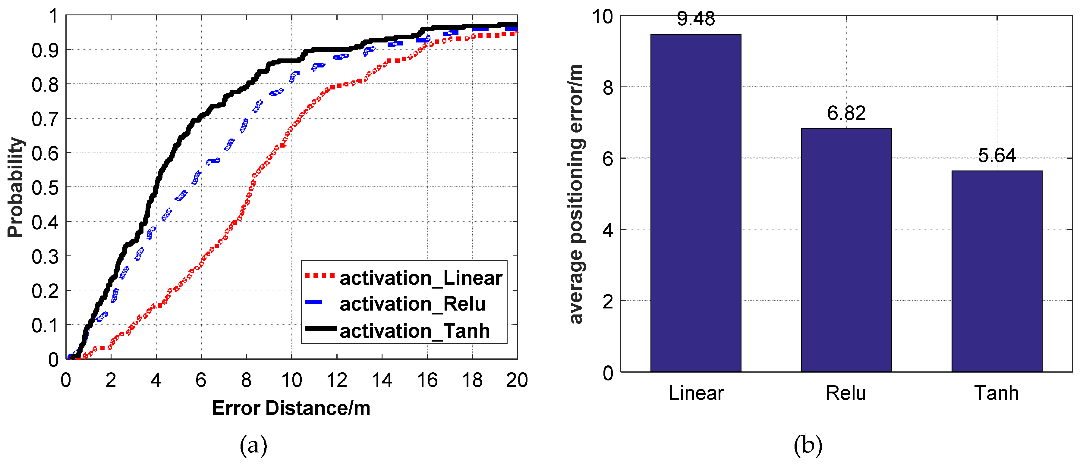
Figure 15.
The positioning accuracy using different activation functions. (a) CDF positioning errors. (b) Average positioning errors.
Figure 15.
The positioning accuracy using different activation functions. (a) CDF positioning errors. (b) Average positioning errors.
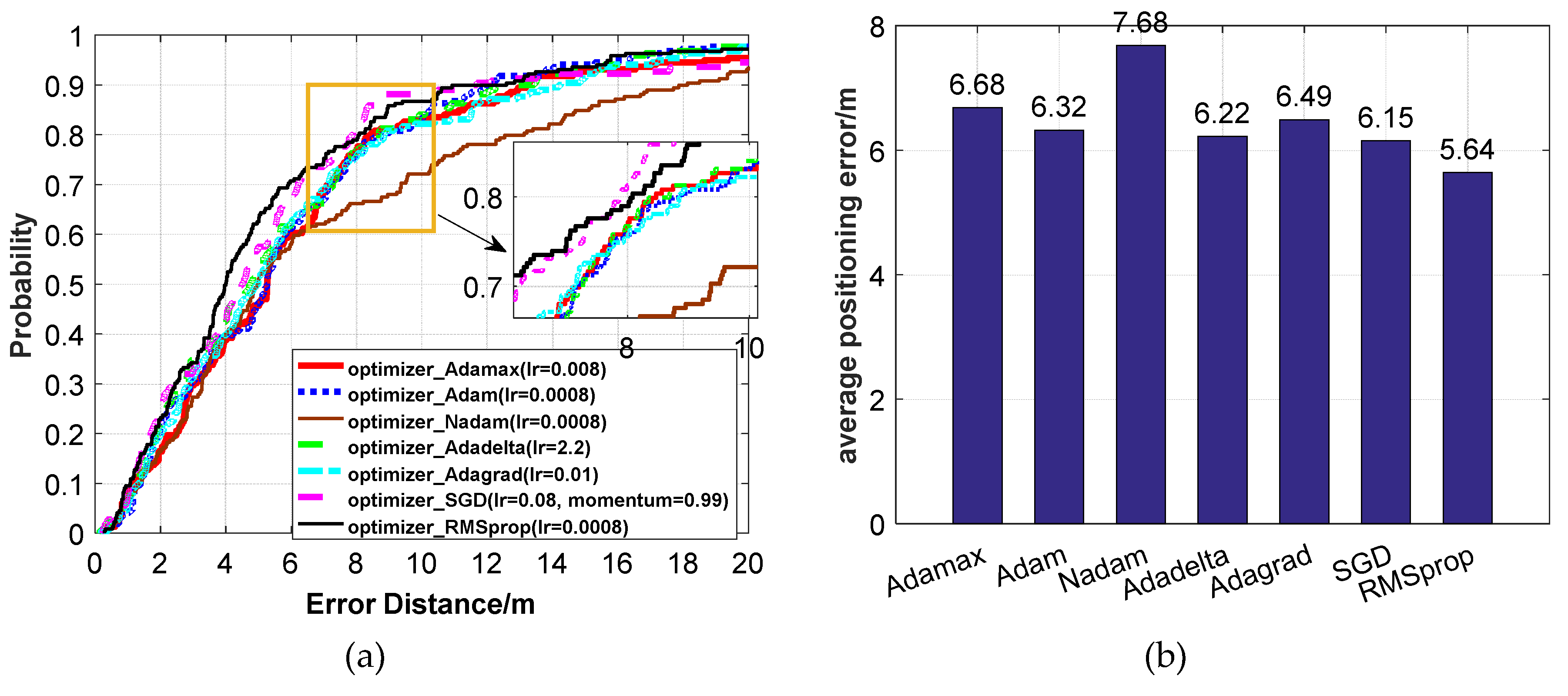
Figure 16.
The positioning accuracy using different optimizers. (a) CDF positioning errors. (b) Average positioning errors.
Figure 16.
The positioning accuracy using different optimizers. (a) CDF positioning errors. (b) Average positioning errors.
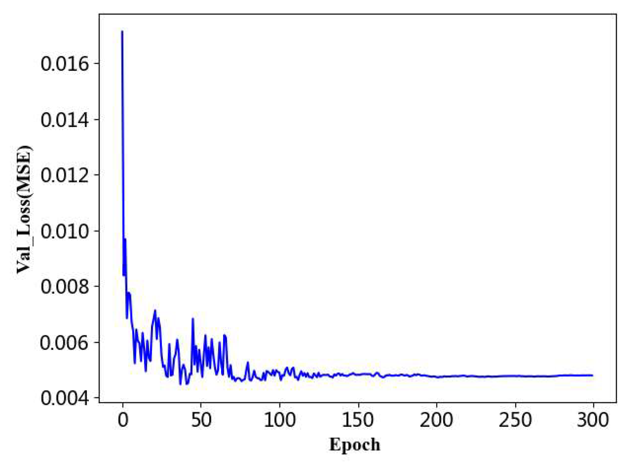
Figure 17.
The loss function declining curve with epoch of the validation dataset.
Figure 17.
The loss function declining curve with epoch of the validation dataset.
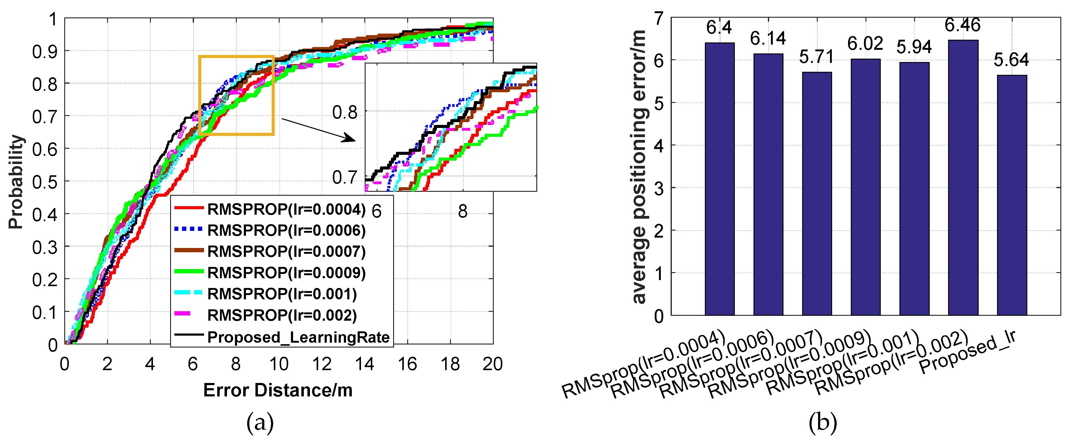
Figure 18.
The positioning accuracy using different learning rates in optimizer (RMSprop). (a) CDF positioning errors. (b) Average positioning errors.
Figure 18.
The positioning accuracy using different learning rates in optimizer (RMSprop). (a) CDF positioning errors. (b) Average positioning errors.
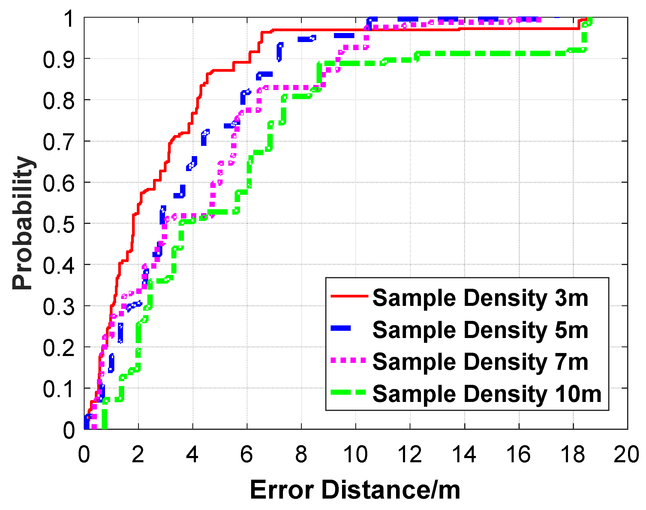
Figure 19.
The CDF positioning error of our proposed algorithm under different sample densities.
Figure 19.
The CDF positioning error of our proposed algorithm under different sample densities.
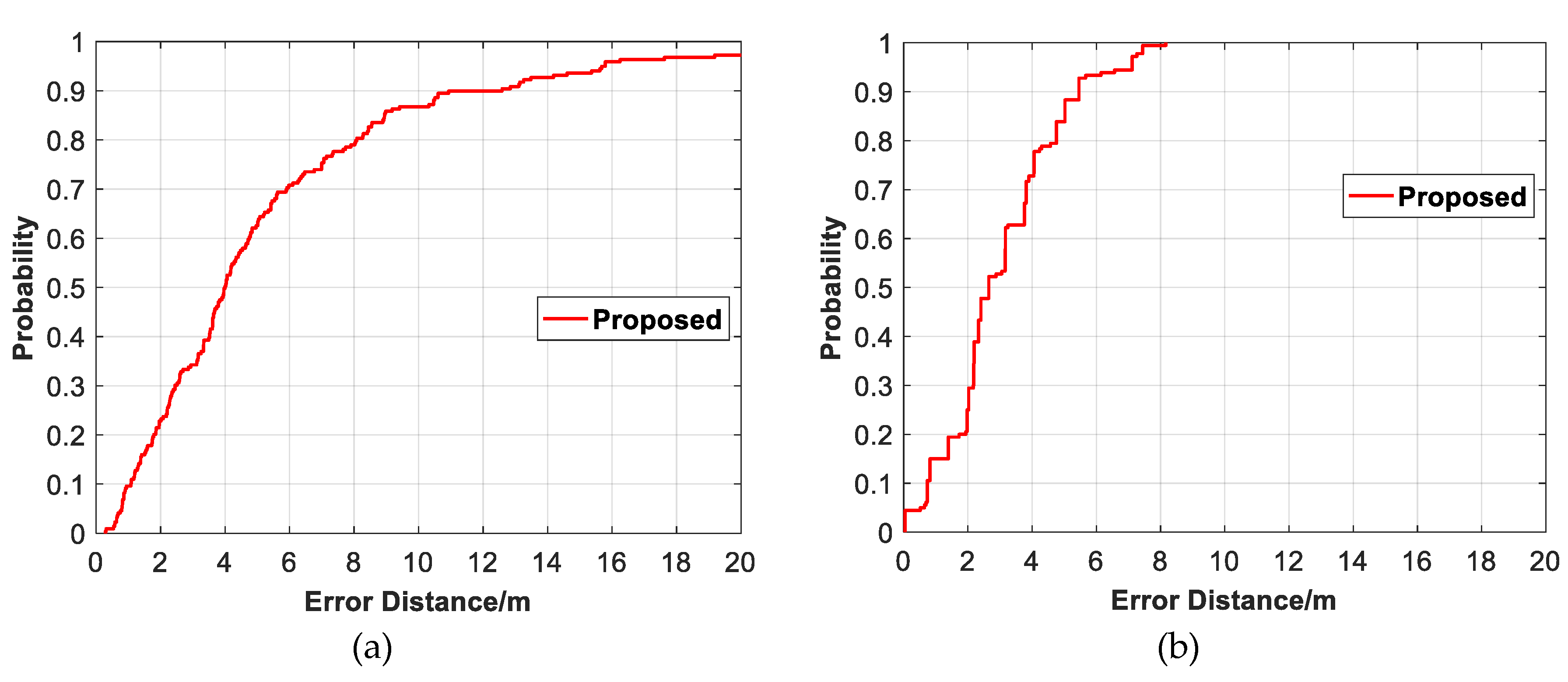
Figure 20.
The CDF positioning error of our proposed algorithm on three datasets. (a) Dataset1. (b) Dataset2. (c) Dataset3.
Figure 20.
The CDF positioning error of our proposed algorithm on three datasets. (a) Dataset1. (b) Dataset2. (c) Dataset3.
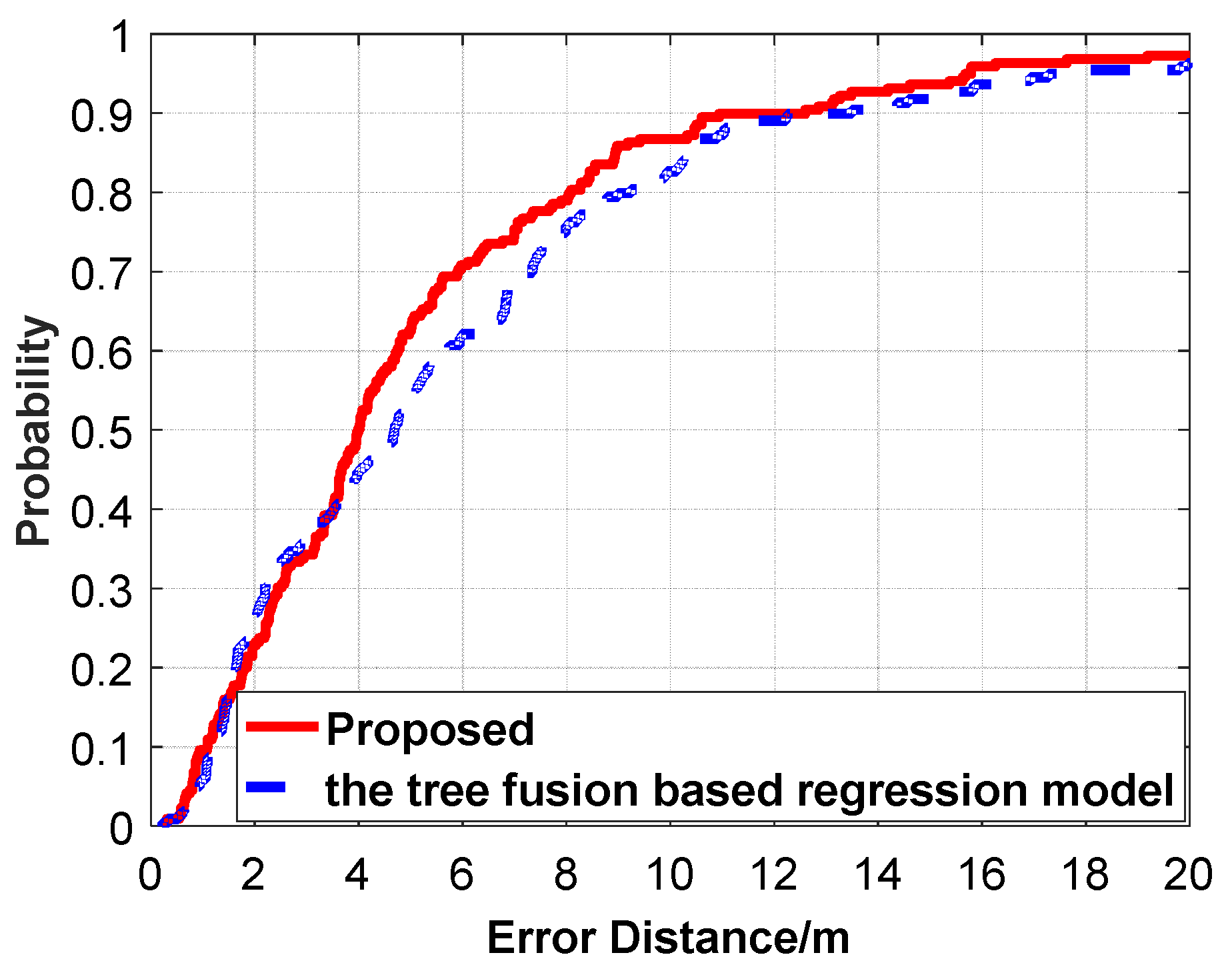
Figure 21.
Comparison of CDF positioning errors between the proposed algorithm and the tree-fusion-based regression model.
Figure 21.
Comparison of CDF positioning errors between the proposed algorithm and the tree-fusion-based regression model.
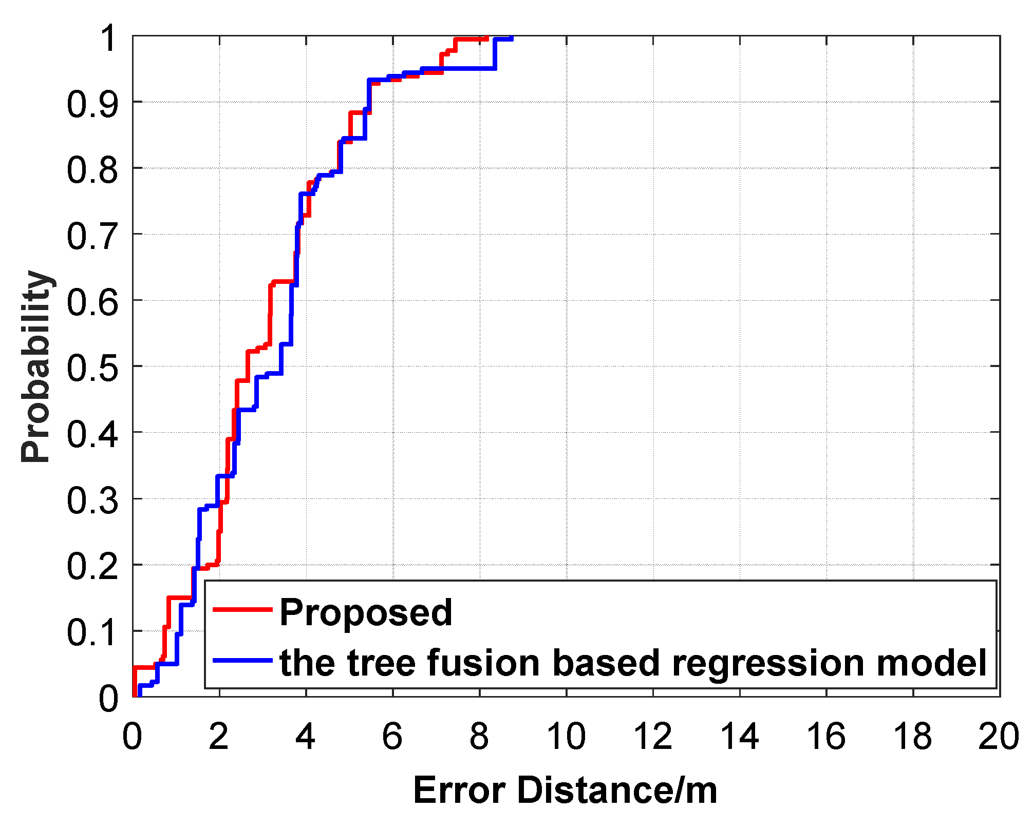
Figure 22.
The positioning errors (CDF) between the proposed algorithm and the tree-fusion-based regression model.
Figure 22.
The positioning errors (CDF) between the proposed algorithm and the tree-fusion-based regression model.
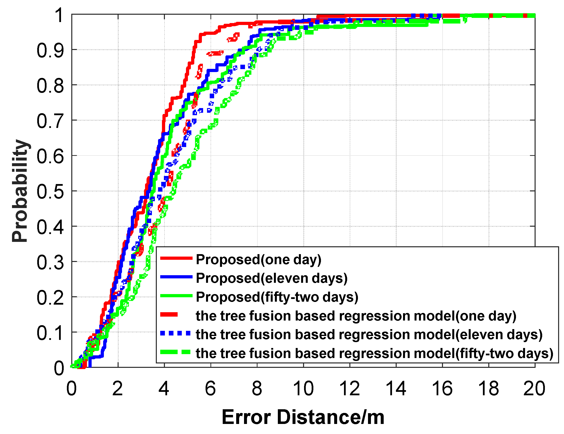
Figure 23.
Comparison of CDF positioning errors between the proposed algorithm and the tree-fusion-based regression model.
Figure 23.
Comparison of CDF positioning errors between the proposed algorithm and the tree-fusion-based regression model.
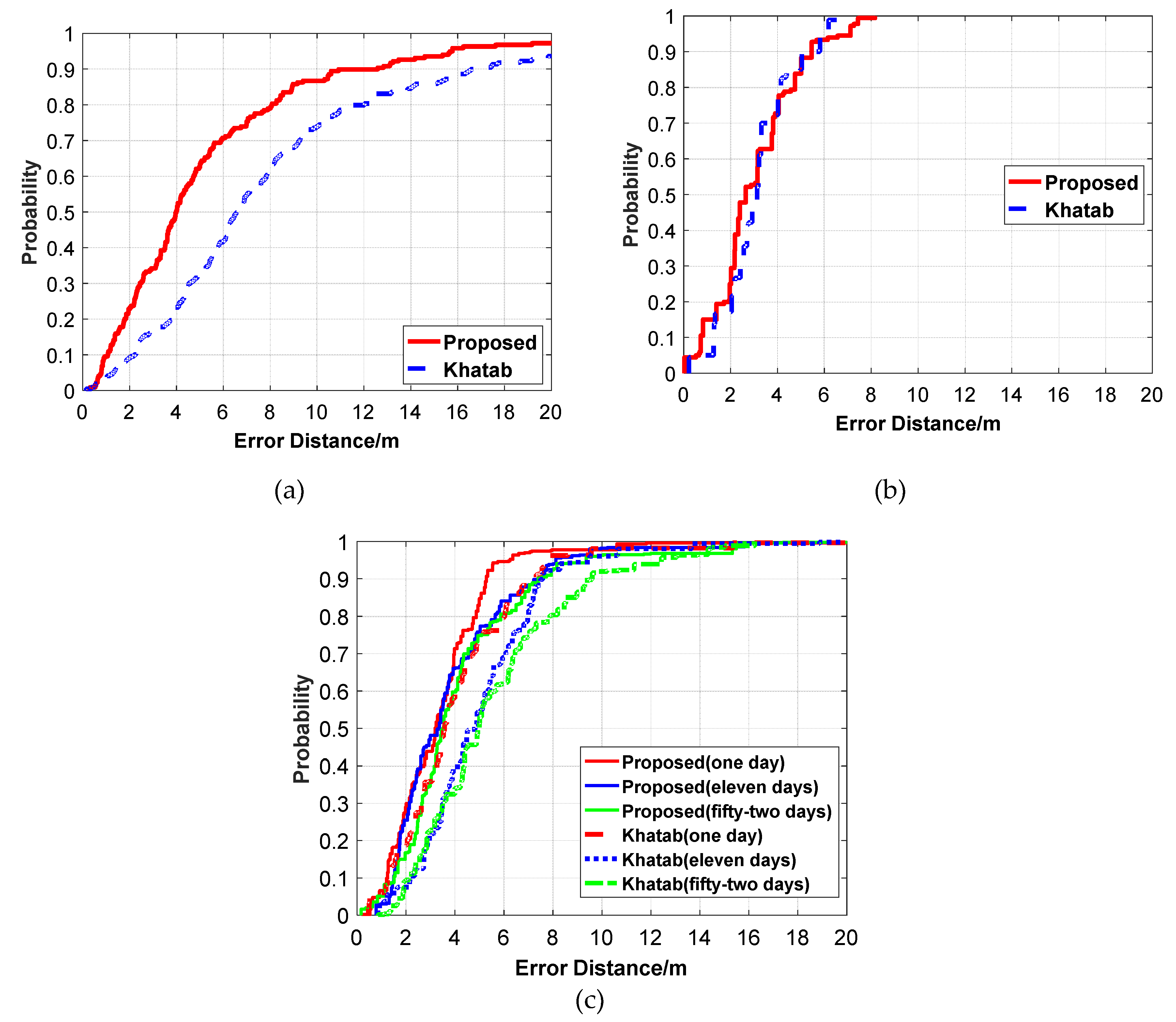
Figure 24.
The positioning error comparison between our proposed algorithm and Khatab’s method on three different datasets. (a) Dataset1. (b) Dataset2. (c) Dataset3.
Figure 24.
The positioning error comparison between our proposed algorithm and Khatab’s method on three different datasets. (a) Dataset1. (b) Dataset2. (c) Dataset3.
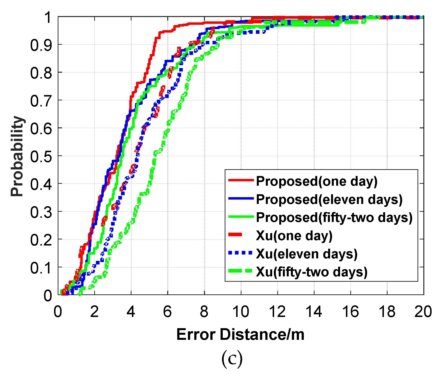
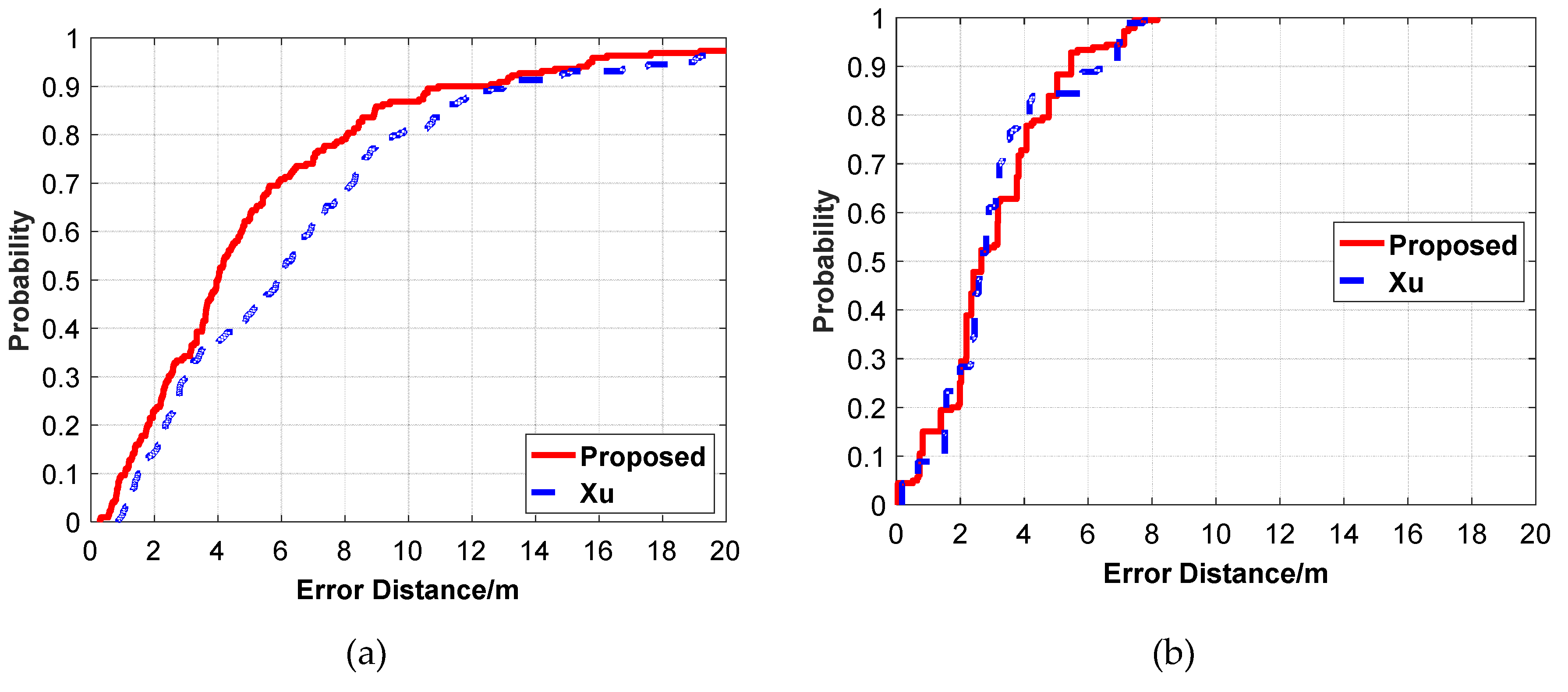
Figure 25.
Comparison of CDF positioning errors between the proposed algorithm and Xu on different datasets. (a) Dataset1. (b) Dataset2. (c) Dataset3.
Figure 25.
Comparison of CDF positioning errors between the proposed algorithm and Xu on different datasets. (a) Dataset1. (b) Dataset2. (c) Dataset3.
Table 1.
Hyperparameter values in our proposed SDAE and MLP.
Table 1.
Hyperparameter values in our proposed SDAE and MLP.
| Parameter | SDAE | MLP |
|---|
| Batch size | 30 | 100 |
| Activation | Relu [47] | Tanh |
| Optimizer | Adam [49] | RMSprop [50] |
| Learning rate | 0.1 | 0.0008 |
| Epochs | 30 (first DAE), 20 (second and third DAEs) | 200 |
| Loss function | MSE | MSE |
Table 2.
Average positioning error of our proposed algorithm under different sample densities.
Table 2.
Average positioning error of our proposed algorithm under different sample densities.
| Dataset | Neighboring sample_spacing (m) | Mean_error (m) |
|---|
| Sample Density 3 m | 3 | 2.84 |
| Sample Density 5 m | 5 | 3.56 |
| Sample Density 7 m | 7 | 4.18 |
| Sample Density 10 m | 10 | 5.63 |
Table 3.
Average positioning error of the algorithm proposed in this paper on three datasets.
Table 3.
Average positioning error of the algorithm proposed in this paper on three datasets.
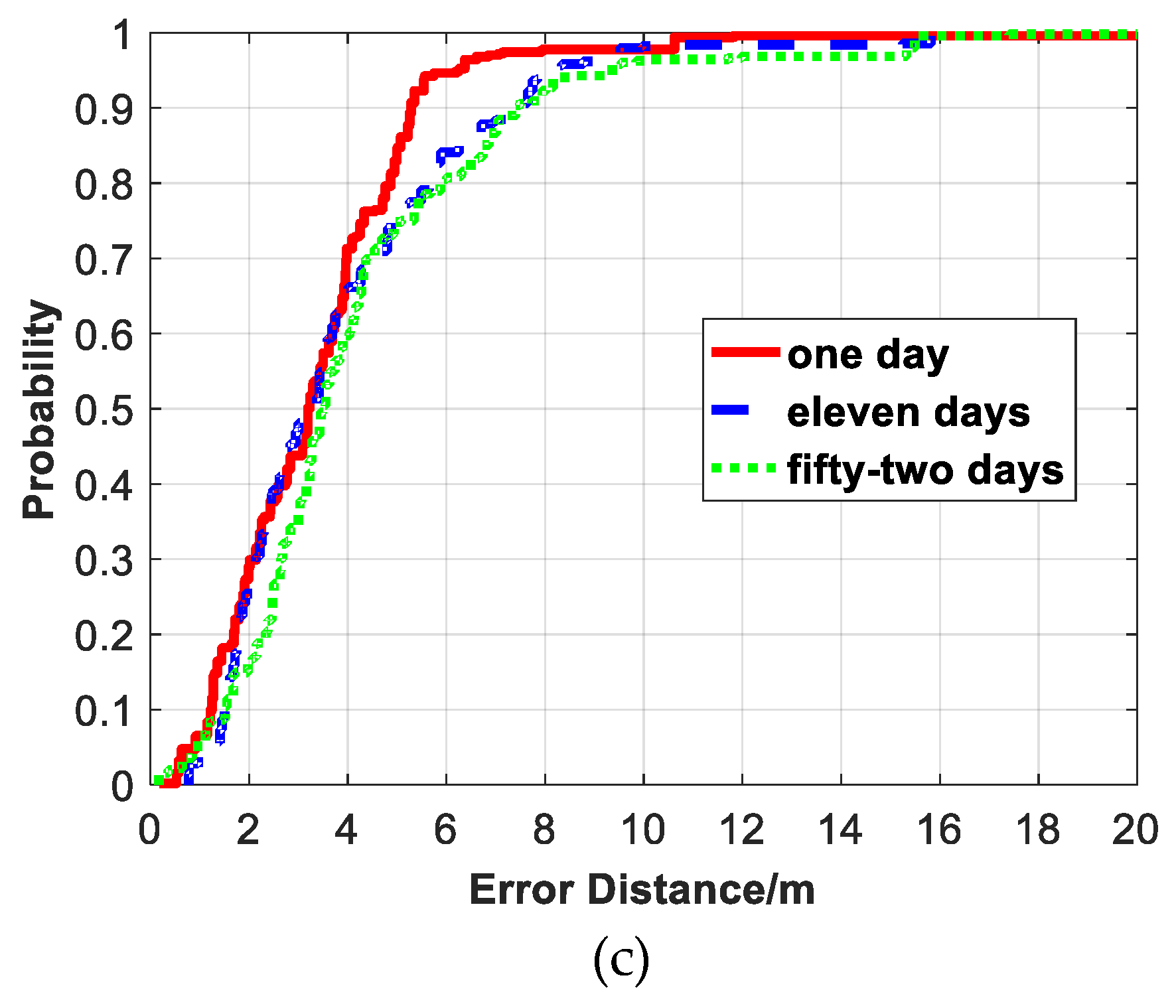
| Dataset | Collection Interval (day) | Mean_error (m) |
|---|
| Dataset1 | 10 | 5.64 |
| Dataset2 | 0 | 3.05 |
| Dataset3 | 1 | 3.39 |
| 11 | 3.85 |
| 52 | 4.24 |
Table 4.
Average positioning errors of the proposed algorithm and the tree-fusion-based regression model.
Table 4.
Average positioning errors of the proposed algorithm and the tree-fusion-based regression model.
| Model | Mean_error (m) |
|---|
| tree-fusion-based regression model | 6.32 |
| Proposed model | 5.64 |
Table 5.
The average positioning error comparison between the proposed algorithm and the tree-fusion-based regression model.
Table 5.
The average positioning error comparison between the proposed algorithm and the tree-fusion-based regression model.
| Model | Mean_error (m) |
|---|
| tree-fusion-based regression model | 3.22 |
| Proposed model | 3.05 |
Table 6.
Comparison of average positioning errors between the proposed algorithm and the tree-fusion-based regression model.
Table 6.
Comparison of average positioning errors between the proposed algorithm and the tree-fusion-based regression model.
| Model | Collection Interval (day) | Mean_error (m) |
|---|
| Proposed model | 1 | 3.39 |
| tree-fusion-based regression model | 4.19 |
| Proposed model | 11 | 3.85 |
| tree-fusion-based regression model | 4.54 |
| Proposed model | 52 | 4.24 |
| tree-fusion-based regression model | 4.97 |
Table 7.
The average positioning errors between our proposed algorithm and Khatab’s method.
Table 7.
The average positioning errors between our proposed algorithm and Khatab’s method.
| Dataset | Model | Collection Interval (day) | Mean_error (m) |
|---|
| Dataset1 | Khatab [30] | 10 | 8.14 |
| proposed | 10 | 5.64 |
| Dataset2 | Khatab [30] | 0 | 3.14 |
| proposed | 0 | 3.05 |
| Dataset3 | Khatab [30] | 1 | 4.08 |
| 11 | 5.01 |
| 52 | 5.60 |
| proposed | 1 | 3.39 |
| 11 | 3.85 |
| 52 | 4.24 |
Table 8.
Comparison of the average positioning errors between the proposed algorithm and Xu.
Table 8.
Comparison of the average positioning errors between the proposed algorithm and Xu.
| Dataset | Model | Collection Interval (Day) | Mean_error (m) |
|---|
| Dataset1 | Xu [31] | 10 | 7.00 |
| proposed | 10 | 5.64 |
| Dataset2 | Xu [31] | 0 | 3.07 |
| proposed | 0 | 3.05 |
| Dataset3 | Xu [31] | 1 | 4.30 |
| 11 | 4.86 |
| 52 | 5.67 |
| proposed | 1 | 3.39 |
| 11 | 3.85 |
| 52 | 4.24 |
Table 9.
Calculation time of different algorithms.
Table 9.
Calculation time of different algorithms.
| Model | Total Training Time (s) | Prediction Time for One Sample (ms) |
|---|
| proposed | 20.84 | 181 |
| Khatab | 5.21 | 3 |
| Xu | 16.54 | 166 |


