High Spatial Resolution Modeling of Climate Change Impacts on Permafrost Thermal Conditions for the Beiluhe Basin, Qinghai-Tibet Plateau

Abstract

Permafrost is degrading on the Qinghai-Tibet Plateau (QTP) due to climate change. Permafrost degradation can result in ecosystem changes and damage to infrastructure. However, we lack baseline data related to permafrost thermal dynamics at a local scale. Here, we model climate change impacts on permafrost from 1986 to 2075 at a high resolution using a numerical model for the Beiluhe basin, which includes representative permafrost environments of the QTP. Ground surface temperatures are derived from air temperature using an n-factor vs Normalized Differential Vegetation Index (NDVI) relationship. Soil properties are defined by field measurements and ecosystem types. The climate projections are based on long-term observations. The modelled ground temperature (MAGT) and active-layer thickness (ALT) are close to in situ observations. The results show a discontinuous permafrost distribution (61.4%) in the Beiluhe basin at present. For the past 30 years, the permafrost area has decreased rapidly, by a total of 26%. The mean ALT has increased by 0.46 m. For the next 60 years, 8.5–35% of the permafrost area is likely to degrade under different trends of climate warming. The ALT will probably increase by 0.38–0.86 m. The results of this study are useful for developing a deeper understanding of ecosystem change, permafrost development, and infrastructure development on the QTP.

1. Introduction

Climate warming rates at high latitudes and high altitudes are greater than the global average [1,2,3]. This warming has produced many changes to the cryosphere, including the permafrost, as evidenced by permafrost temperature increases and positive trend of the active-layer thickness [4]. Most future projections with climate models suggest continuous warming, which will further induce a reduction of the global permafrost by between 30% and 70% until 2100 [5]. Permafrost degradation is likely to have wide-ranging influences on surface and subsurface hydrologic conditions, soil strength properties and ecosystems [6]. The Qinghai-Tibet Plateau (QTP) is the largest lower latitude permafrost region in the world. During the last decades, permafrost warming has been widely reported, according to the measurements of permafrost temperatures in boreholes on the QTP [7,8,9,10]. Changes in the active-layer thickness and permafrost temperature due to climate warming affects infrastructure, ecosystems [11,12], and the stability of slopes [13] on the QTP. Ongoing climate change and its associated effects on ground thermal dynamics, and natural hazards make it important to assess spatial permafrost thermal dynamics on the QTP. Presently, the available permafrost thermal maps (ground temperature, and active-layer thickness maps) are mainly at low resolutions or do not assess the permafrost dynamics over time [14,15,16,17], although many permafrost maps have been compiled since the early 1960s [18]. In addition, some promising empirical approaches are limited by methodology, assumptions and availability of true ground information. Therefore, improved methods for modeling spatial permafrost thermal dynamics at the local scale are essential for land use decisions, ecological impact assessment, and providing robust boundary conditions for climate models on the QTP.

Numerical permafrost models based on conductive heat transfer have proven to be powerful tools for estimating the spatial thermal distribution of permafrost and its changes following climate change [19,20,21]. These models require detailed input data, such as surface meteorological variables, and soil thermal parameters, to simulate and forecast the thermal regime of permafrost over a relatively short time interval at a high resolution. Input datasets can be derived from a number of sources, for example, in situ measurements of soil temperature and air temperature, and satellite data which has been extensively used in permafrost modeling [22,23,24,25].

The study area for this paper is the Beiluhe basin in the central QTP (Figure 1). This basin is a significant region for permafrost research on the QTP, including the permafrost temperature [26], thermokarst lake dynamics [27,28], and carbon dioxide and methane feedback [29]. Therefore, the permafrost’s extent and characteristics and its response to climate change are of major concern, but the present knowledge is still very limited. In this region, detailed in-situ measurements of meteorological variables and the ground temperature are readily available [26,30], so that the area constitutes an ideal region to assess the performance of thermal permafrost modeling at the local scale. The objectives of this study are (i) to develop an approach to model and map the permafrost thermal regimes at a high spatial resolution; and (ii) to further investigate and quantify permafrost thermal dynamics with climate change.

2. Methods and Data

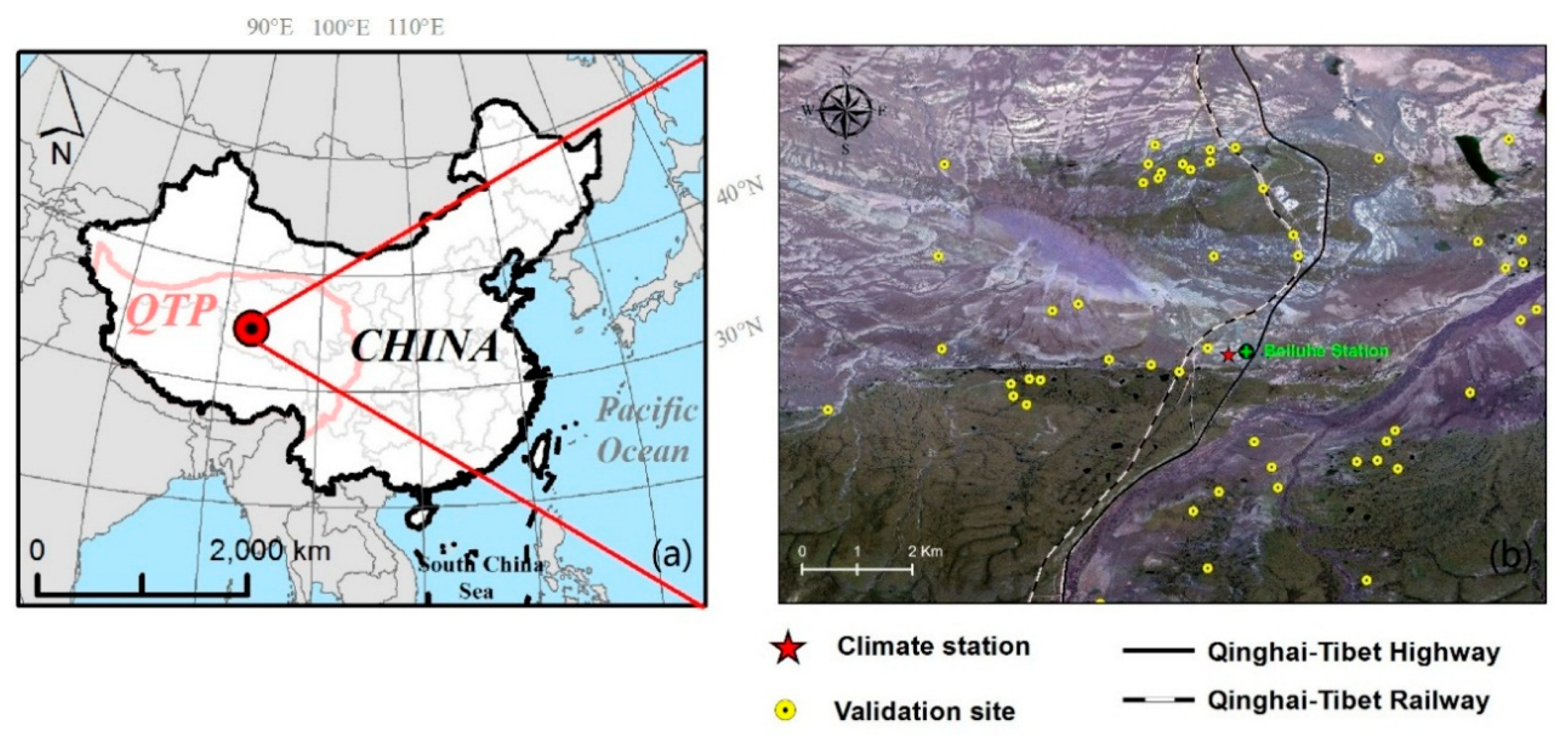
2.1. Study Area and Field Data Acquisitions

The study area (around 130 km²) is in the Beiluhe basin, which is located in the central QTP (Figure 1). This region is relatively flat, with an average elevation of 4628 m a.s.l. This study area is dominated by discontinuous permafrost in an extremely continental climate [14], with a mean annual air temperature (MAAT) of –3.4 °C and annual total precipitation of 369.8 mm, over 90% of which falls as rainfall during summer [26]. The mean annual ground temperature (MAGT) is between –1.5 °C and 0 °C, and the active-layer thicknesses (ALT) ranges from 1.4 m to 3.4 m [26]. According to detailed investigations by Yin et al. [26], this area can be classified into 10 ecotypes, which have distinctly different characteristics regarding their surface and subsurface properties, such as vegetation cover, water bodies and ground ice contents (

Table 1. Ground surface type and associated soil type in the study area [26].

Class ID	Surface Type	Soil Texture	Class ID	Vegetation	Soil Texture
1	Swamp meadow	Fine sand	6	Sparse grassland	Sand with gravel
2	Undisturbed alpine meadow	Fine sand	7	Bare ground	Stone and gravel
3	Degrading alpine meadow	Fine sand	8	Water body	--
4	Alpine steppe	Sand with gravel	9	Water	--
5	Desert alpine grassland	Sand	10	Bare ground	Aeolian sand

). There are five vegetation types in this region: swamp meadow, undisturbed alpine meadow, degrading alpine meadow, alpine steppe, and desert and sparse grassland.

Four major field data sources are used for this study. One is the thermal boreholes across this region (2006–2016), reported by Yin et al. [26], which provide general information about the permafrost temperature and ALT, geology, geomorphology, and soil hydrology. The ALT is calculated based on the 0 °C isotherm of the ground temperature. The second one is a detailed ecosystem classification of the area, using supervised classification method with high-resolution satellite images (Gao fen-1, 2.0 m resolution). The third is the available climate station in this study, which provides general information about the climate (Figure 1b). It records the air temperature (2.0 m above the ground surface) and ground surface temperature every 4 h and has done so for a very long time for a long period (1956–2018). Lastly, soil thermal properties were measured using a portable thermal characteristic analyzer (KD 2 Pro, Washington, DC, USA), with an accuracy of 95% for the volumetric heat capacity (C), 95% for the thermal conductivity (k), and 90% for the thermal diffusivity (D). In a companion study [26], we have shown the field data details and the method of ecosystem classification.

2.2. The GIPL 2.0 Ground Thermal Model

In this study, we make use of the GIPL 2.0 numerical transient model, which is capable of representing the freezing and thawing cycle. This model has been successfully applied to the entire Alaskan [19] and the QTP permafrost region [15]. The ground temperature is calculated by solving the 1-D heat transfer equation, accounting for the phase change of soil water. Heat conduction is assumed as the only process of energy transfer in the model. The volumetric content of liquid water with temperature is the unfrozen water content characteristic curve and it depends on soil composition and structure. The model does not account for changing subsurface water contents, but instead assigns fixed values for the porosity and saturation of each grid cell. The detailed description of this model can be found in Jafarov et al. [19] and Tipenko et al. [31]. The code of the GIPL 2.0 model is available on the GitHub website: https://github.com/Elchin/GIPL.

2.2.1. Model Setting and Boundary Condition

At 2.0 m spatial (horizontal) resolution, the soil and ground profile domain are generated with 139 vertical finite elements to a depth of 100 m. The size of the cells increases with depths with a minimum grid cell spacing of 0.1 cm for shallow soils and maximum spacing of 10 m at the bottom. The soil profile includes fibrous horizons, mineral soils, and bedrock. The upper boundary conditions are determined on time series of the near-surface air temperature, and the lower boundary conditions are defined based on a geothermal gradient of 0.07 °C m⁻¹, as estimated from a deep borehole [32].

2.2.2. Forcing Datasets and Model Initialization

GIPL 2.0 requires a synthesized time series of daily near-surface air temperature as the forcing data sets. Allowing for the effects of the surface conditions on the surface energy balance, the simplistic n-factor is used to predict the ground surface temperature (Equation (1)) [33,34].

$$T_s=\{\begin{array}{l}{n}_f{T}_{air},\mathrm{if}{T}_{air}<0\\ n_t{T}_{air},\mathrm{if}{T}_{air}\ge 0\end{array}$$

(1)

The n values for all vegetation classes are derived from 17 sites measuring daily air and ground surface temperatures (2012–2016) [26]. During winter, the n_f values for swamp meadow, undisturbed alpine meadow, degrading alpine meadow, alpine steppe, and desert grassland are set at a constant of 0.5, 0.7, 0.5, 0.6, and 0.6, respectively [26]. As shown in Figure 2, there is a strong correlation between annual mean n_t values and Normalized Differential Vegetation Index (NDVI) values based on in situ measurements. For each 2.0 m grid cell, the month mean NDVI value is determined from a 0.8 m spatial resolution multi-spectral Gao fen-2 image at noon local time from 1 August to 31 August 2016; this period is based on a cloud free day. The summertime n_t is simulated based on the NDVI of each grid cell using Equation (2).

$$n_t=19.65NDV{I}^2-17.07NDVI+4.78$$

(2)

The forcing data cover a period from 1956 to 2017. Generally, a pronounced increase in air temperature and precipitation started after the 1980s. It is reasonable to presume the climate was steady for a long time before the 1980s [26]. Therefore, the permafrost around the 1980s is assumed to be in equilibrium. To estimate a realistic initial temperature profile, the model is spun up using a repeated 30-year period from 1956 to 1985 with a soil temperature profile (T_i). T_i is obtained by extrapolating the present available initial ground temperature profiles to the region using Kriging interpolation. In order to evaluate the permafrost dynamics, the target periods are divided into five ranges, i.e., 1986 to 1995, 1996 to 2005, 2006 to 2015, 2016 to 2045, and 2046 to 2075. For the next 60 years, a sine function with a constant warming rate for the future near-surface air temperature change is assumed. We consider two warming scenarios with the rates of 0.015 °C yr⁻¹ and 0.065 °C yr⁻¹. The value of 0.065 °C yr⁻¹ represents the average rate of temperature increase, based on field air temperature observations from 1980 to 2017. The value of 0.015 °C yr⁻¹ represents the average rate of increase over the next 60 years based on the objective of the Paris climate agreement [35,36]. In this study, the near surface air temperature is assumed to be uniform across the study area.

2.2.3. Subsurface Properties and Model Parameters

Three soil layers are distinguished according to field investigation [26]. Most of the region is covered by sand and sandy loam with gravel (near surface layer). We define subsurface stratigraphy (intermediate layer) as clay. The bottom mineral layer is defined as rock for the entire study area. Similar to Zhang et al. [21] and Nicolsky et al. [22], we employ the ecosystem types interpreted by Yin et al. [26] to parameterize the thermal properties of the soil texture, excluding rivers and lakes. Based on this ecotype map, we distinguish five soil texture categories as the predominant subsurface stratigraphy within the study area (

Table 2. Parameter values used in ground temperature simulations in each ecotype for each soil layer given. VWC = volumetric water content (fraction of 1); UWC = unfrozen water coefficients; C_t/C_f = thawed/frozen volumetric heat capacities; k_t/k_f = thawed/frozen thermal conductivities.

Soil Layer	VWC	UWC		C (106 J m−3) K−1)		K (W m−1 K−1)		Depth (m)
		a	b	Ct	Cf	kt	kf
Swamp Meadow
Sand	0.20	0.07	−0.17	3.1	1.5	1.5	0.9	0–1
Clay	0.18	0.12	−0.15	2.5	1.9	1.7	2.2	1–10
Rock	0.04	0.01	−0.1	3.25	2.48	2.7	3.1	>10
Undisturbed Alpine Meadow
Sand	0.18	0.07	−0.17	3.1	1.5	1.6	2.4	0–2
Clay	0.17	0.12	−0.15	2.5	1.9	0.7	1.4	2–10
Bedrock	0.04	0.01	−0.10	3.25	2.48	2.7	3.1	>10
Degrading Alpine Meadow
Sand	0.06	0.037	−0.14	2.8	2.2	1.3	1.6	0–2
Clay	0.12	0.12	−0.15	2.5	1.9	1.3	1.6	2–10
Rock	0.04	0.01	−0.10	3.25	2.48	2.7	3.1	>10
Alpine Steppe
Sand with gravel	0.12	0.037	−0.14	2.8	2.2	1.3	1.6	0–3
Clay	0.12	0.12	−0.15	2.5	1.9	0.6	1.0	3–10
Rock	0.04	0.01	−0.1	3.25	2.48	2.7	3.1	>10
Desert Grassland
Sand	0.1	0.05	−0.17	3.1	1.5	1.3	1.6	0–5
Clay	0.12	0.12	−0.15	2.5	1.9	0.6	1.0	5–10
Rock	0.04	0.01	−0.1	3.25	2.48	2.7	3.1	>10

). The 2.0 m resolution land cover map delineates local-scale ecosystems that partition geomorphic, hydrologic, pedologic, and vegetative characteristics of the land. Therefore, after combinations of the land-cover types and mineral soil types are decided, ground thermal properties for each cell are defined based on the field measurements (Table 2).

In addition, the near surface conditions (vegetation, landscape) and underground (soil condition) are assumed to be constant during the simulation periods, as the land cover map was made from Gao fen-1 and Gao fen-2 images which can only be acquired from 2015 and 2016.

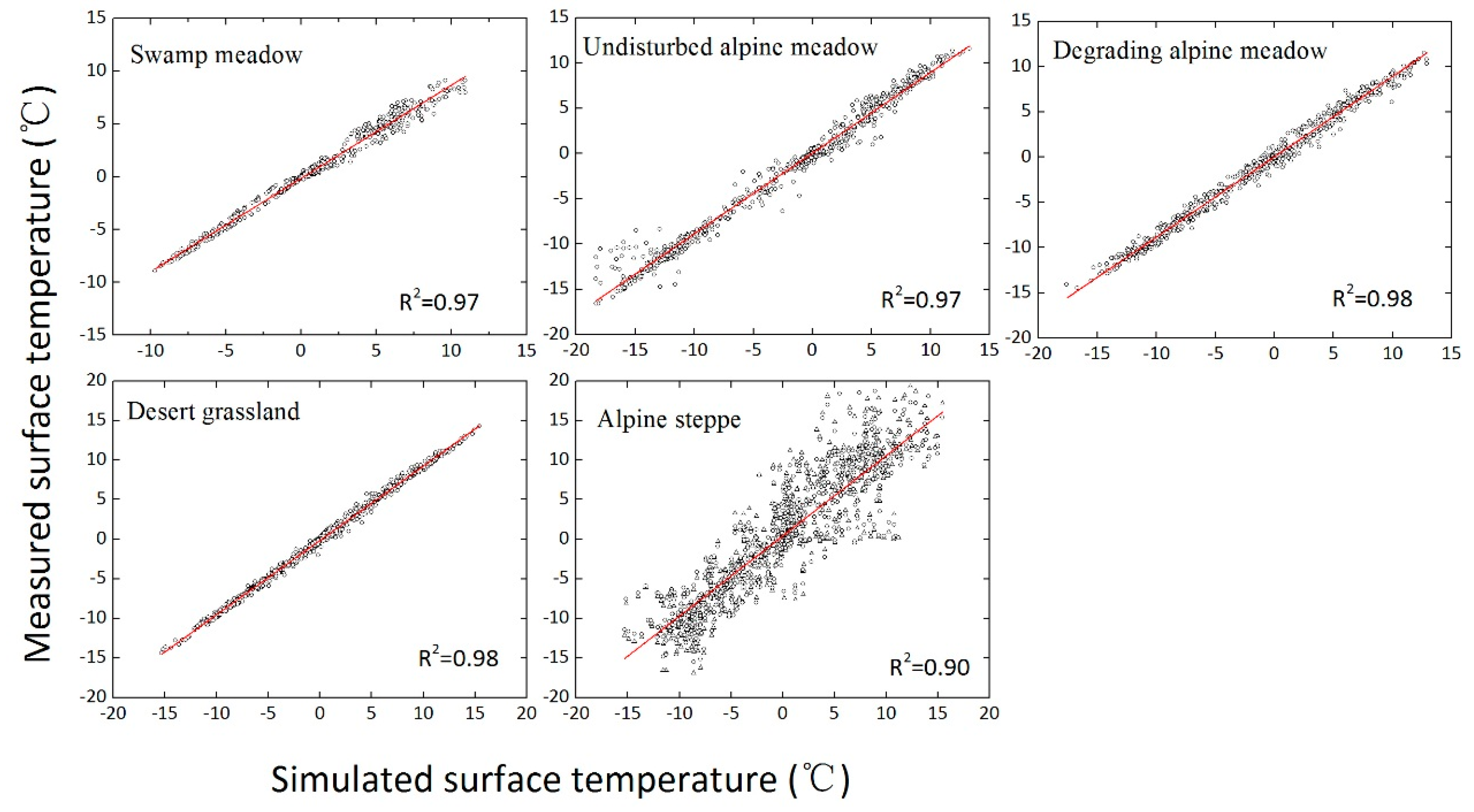
2.2.4. Model Calibration and Validation

Site-based calibration and validation is conducted for different vegetation covered areas. As shown in Section 2.2.2, the model is initialized using the climate data in 1956 and then the model is run from 1956 to 2016. The outputs of the model are compared with field observations based on the data availability (2002–2016). An iterative procedure is applied to recalibrate the parameters until a satisfactory goodness of fit between the observed and modelled soil temperatures is obtained.

Figure 3 shows the comparison between simulated and measured daily ground surface temperatures at different sites. The correlation coefficients (R²) are generally above 0.9.

Table 3. Statistics of the measured and simulated mean annual ground temperature (MAGT) at different depths. ME = mean error; MAE = mean absolute error; RMSE = root mean square error; R² = coefficient of determination; N = day.

Site	Depth (m)	R2	ME	MAE	RMSE	N
Swamp Meadow	0.3	0.95	0.8	1.1	2.4	708
	3.0	0.92	0.1	0.1	0.3	708
	5.0	0.93	0.1	0.1	0.2	708
	10.0	0.94	0.0	0.1	0.2	708
Undisturbed Alpine Meadow	0.3	0.98	0.8	1.1	2.4	708
	3.0	0.98	0.1	0.1	0.3	708
	5.0	0.97	0.1	0.1	0.2	708
	10.0	0.93	0	0.1	0.2	708
Degrading Alpine Meadow	0.3	0.98	−0.5	0.8	1.8	712
	3.0	0.95	0.0	0.2	0.2	712
	5.0	0.95	0.0	0.1	0.0	712
	10.0	0.73	0.0	0.0	0.0	712
Alpine Steppe	0.3	0.88	1.1	0.6	1.2	708
	3.0	0.90	0.8	0.8	0.5	708
	5.0	0.92	0.3	0.2	0.1	708
	10.0	0.9	0.1	0.1	0.2	708
Desert Grassland	0.3	0.95	−0.1	0.6	0.8	697
	3.0	0.85	0	0.1	0.1	697
	5.0	0.92	0	0.1	0.1	697
	10.0	0.92	0	0.1	0.1	697

shows the statistical analysis related to the comparison between the simulations and the observations at different depths. The statistics indicate that the simulated MAGTs are close to the field observations. Most of the R² values are above 0.9, and the mean absolute errors (MAE) are generally below 1.0 °C. A scatterplot of simulated and observed ALTs (30 sites) shows a good correlation (R² = 0.87), although there are some bias errors (mean bias error < 0.25 m) in different geomorphological units (Figure 4). Therefore, the simulated ALT and MAGT are in good agreement with the in situ measurements, indicating the validity of the GIPL 2.0 model for obtaining the ALT and permafrost thermal state in this study.

3. Results

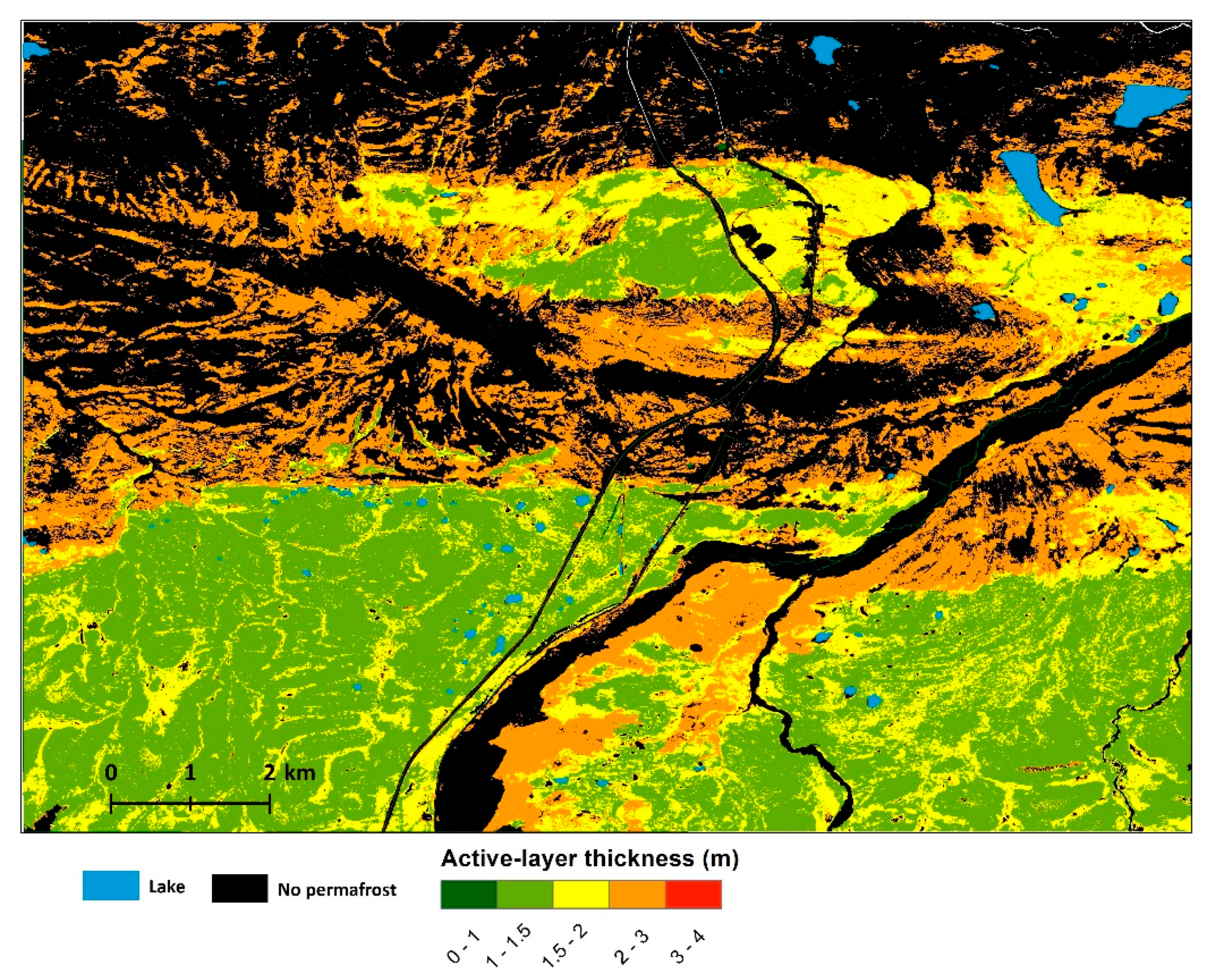
3.1. Present Permafrost Distribution

Figure 5 and Figure 6 present the modeled average ground temperatures (MAGT) and active-layer thickness (ALT) for the period of 2006–2015 at a grid resolution of 2.0 m, excluding the water bodies. The MAGT values are relatively high as modelled mostly between −2.0 °C and 0 °C. The lowest MAGTs (< −1.5 °C) are found in the swamp meadow and undisturbed alpine meadow areas, and the highest MAGTs with a temperature above 0 °C are found in the alpine steppe and desert grassland areas. For alpine meadow (i.e., undisturbed alpine meadow and degrading alpine meadow) areas, the relatively warm MAGTs, ranging from −1.5 °C to 0 °C, are modeled. Considering a MAGT = 0 °C as the threshold for permafrost occurrence, the permafrost covers about 61.4% (81 km²) of the study area, excluding rivers and lakes (8.8% of the area). Therefore, the permafrost extent in our study is discontinuous (underlying 50–90% of the landscape). Generally, permafrost areas with a colder MAGT have relatively thinner ALTs, while the areas with warmer MAGTs are covered by thicker ALTs (Figure 6). In swamp meadow and undisturbed alpine meadow, average ALTs of less than 2.0 m are modeled, while degrading alpine meadow features ALTs of 2.0–3.0 m. For alpine steppe and desert grassland where sporadic permafrost exists, the modeled average ALTs generally range from 2.0 m to 4.0 m.

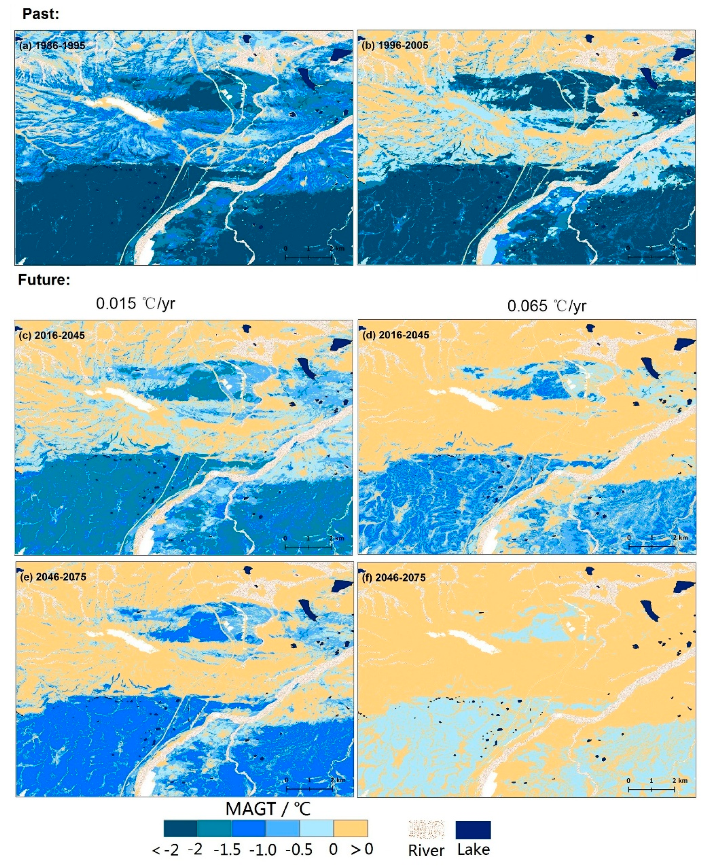
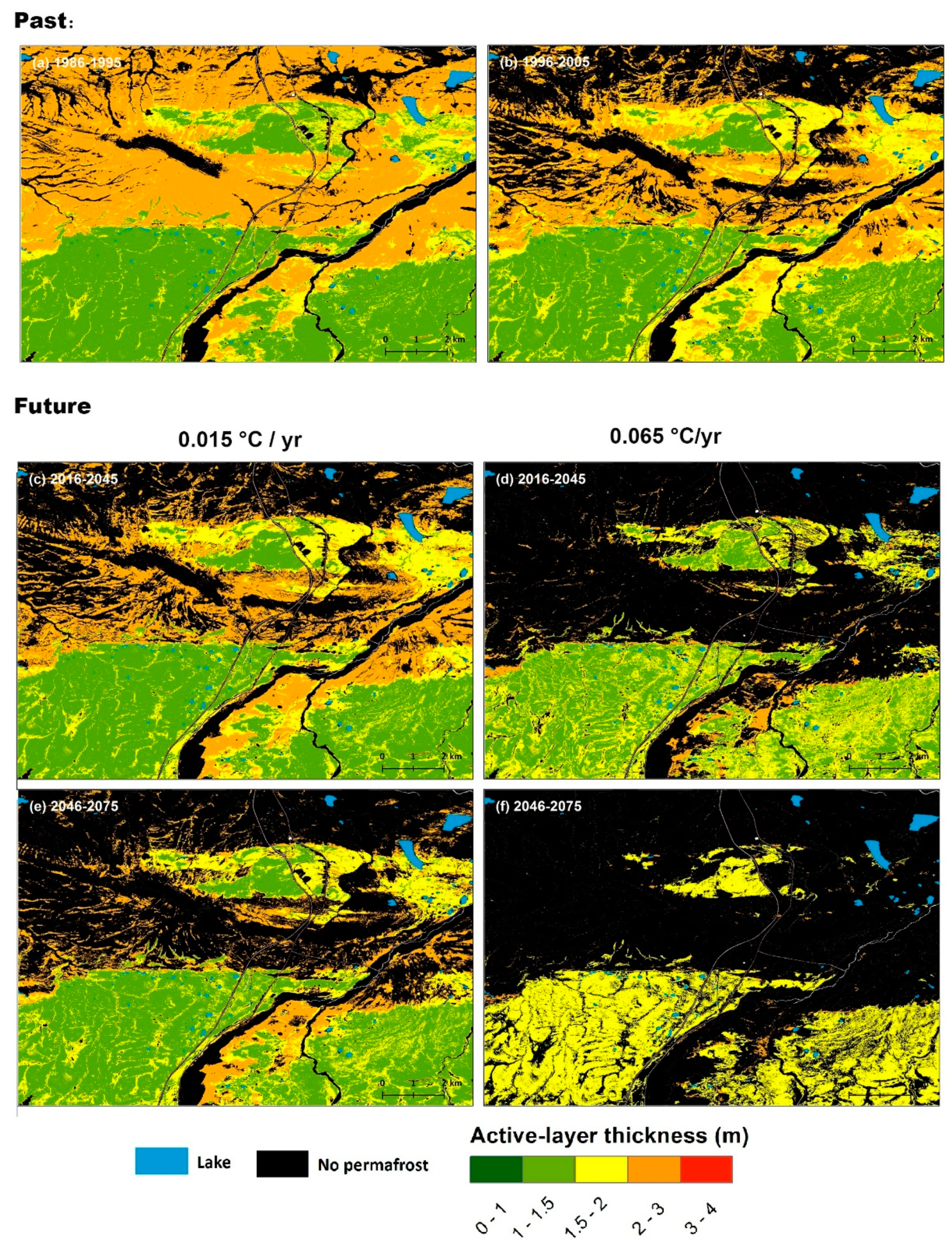
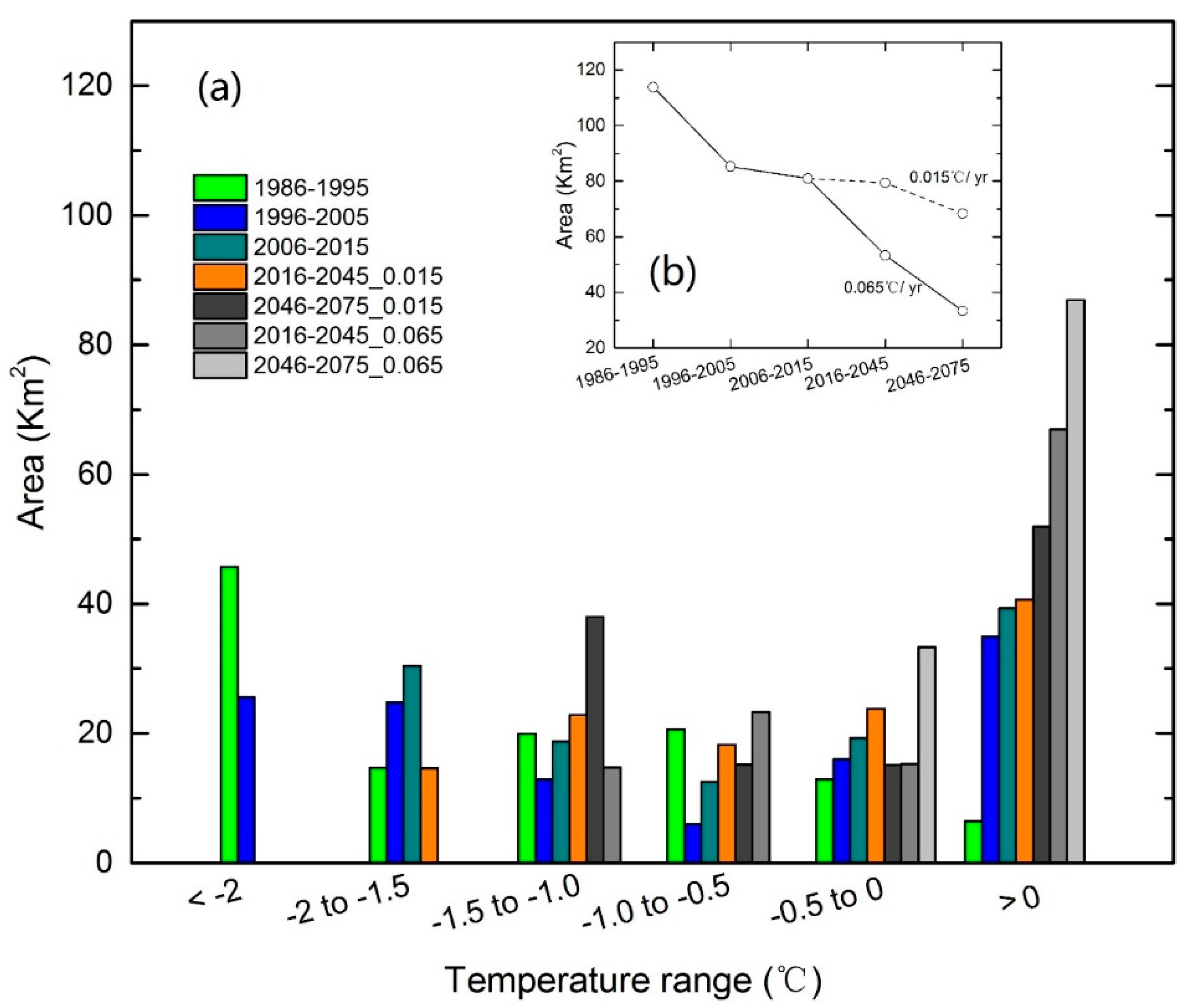
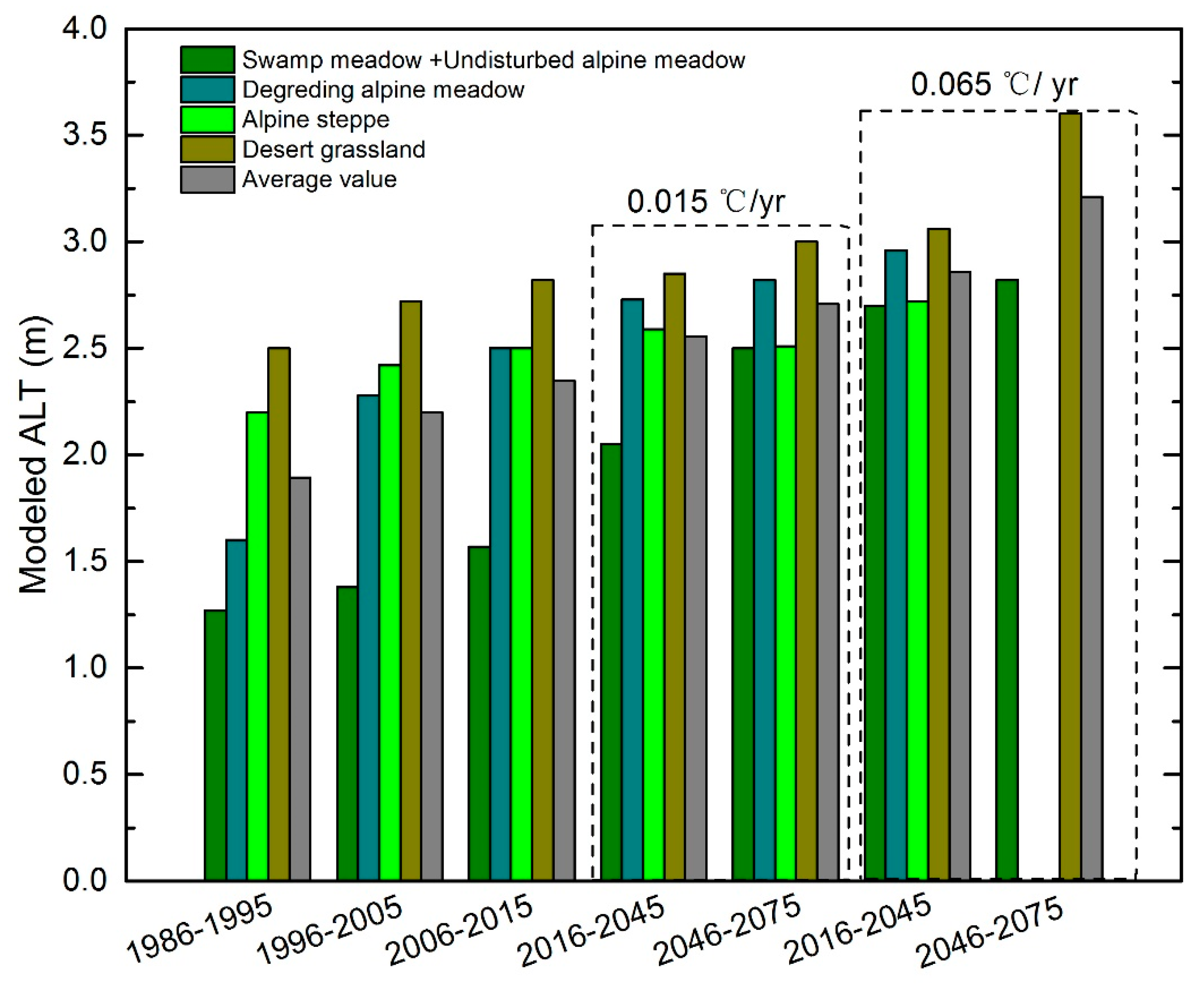
3.2. Historic and Future Permafrost Development in a Warming Climate

Figure 7 and Figure 8 depict the spatial distribution of the MAGT and ALT for the periods of 1986–1995, 1996–2005, 2016–2045, and 2046–2075, respectively. Figure 7a,b shows the evolution of the permafrost temperature during the past 20 years. In the 1990s (i.e., 1986–1995), permafrost existed in most area (occupying about 86.3% of the region, Figure 8b), with most MAGT values being < −1.5 °C (Figure 8a). The permafrost area extent decreased rapidly by 26% to 60.3% in the 2000s (i.e., 1996–2005) (Figure 8b). The area covered by MAGT values of < −2.0 °C has disappeared over the last 30 years. Given the variations of climate change in the next 60 years, the overall area covered by MAGT values of <0 °C is going to decrease at different rates. According to the simulations, in the following 30 years and 60 years: (i) if the climate continues with the current warming trend (0.065 °C yr⁻¹), the area covered by permafrost will decrease rapidly to 40.4% and 25.3%, respectively; while (ii) if the climate warming rate is going to be lower (0.015 °C yr⁻¹), the area covered by permafrost will slightly decrease to 64.7% and 51.8%, respectively. MAGT changes will be much more pronounced within the areas covered by colder permafrost (MAGT< −1.5 °C) in comparison with areas where the permafrost temperature is presently close to 0 °C. The modeled average ALT for the permafrost domain also shows a significant response to scenarios of climate change (Figure 9). As shown in Figure 10, in the last 30 years, the ALTs have been modeled as generally 1.0–1.5 m in the swamp meadow and undisturbed alpine meadow areas, and 1.5–2.0 m in degrading alpine meadow areas. For the desert grassland and alpine steppe, the ALTs range from 2.0 m to 3.0 m. On average for the entire region, the ALT increased by 0.46 m from the 1990s (i.e., 1986–1995) to the 2010s (i.e., 2006–2015). The major changes in ALT occurred in degrading alpine meadow. From the 2010s to the end of the 21st century (2046–2075), the average ALT will increase by 0.38 m and 0.86 m under the scenarios of 0.015 °C yr⁻¹ and 0.065 °C yr⁻¹, respectively (Figure 10).

4. Discussion

4.1. Model Uncertainties

In this study, the spatial n-factors and soil thermal parameters are scaled up from point observations by using high-resolution satellite images. The ground surface temperature is driven from the air temperature based on an NDVI versus n-factor relationship (Equation (2)). One of the major uncertainties is related to this relationship, although this approach has been applied in recent permafrost modeling studies [33,34,37]. The summer n-factor (n_t) had large variations even in a short time scale and among different ground surface types, and the winter n-factor (n_f) had a relatively smaller variation with the time series [26,38]. In this study, we acknowledge that the quantitative error of using this relationship (Equation (1)) to represent the historic and future period is not able to be analyzed due to the lack of long-term available field data and robust prediction of ecosystem dynamics. However, Hipp et al. [34] analyzed the bias error caused by n-factor variations, and indicated that a carefully verified n-factor is a good representation of the long-term average n-factor. This study is focused on the seasonal or multi-annual average ground temperature (i.e., MAGT) and ALT. In addition, employing the n-factor rather than more physical or quasi-physical approaches can reduce the sensitivity of the model to the parameters [39]. The good agreement of the modelled results with the measured MAGT and ALT makes us confident that the simplistic n-factor approach is valid in the model runs.

Another major uncertainty is the information about the soil thermal parameters which may differ within an ecosystem type. In this study, both soil water and ice content are assumed to be constant, neglecting both long-term changes in the water cycle and lateral variations. Ground thermal properties, especially related to hydrogeologic ones, are proven to be the main source of model uncertainty regarding modeled permafrost temperature and thaw depth at a local scale [22,40,41]. Lateral heat flux or subsidence due to ground ice melt can modify the ground thermal regime [42]. Changes in vegetation composition due to soil water condition change driven by permafrost thaw are widely observed in permafrost domain [43,44,45]. Additionally, climate change and human disturbances have significant impacts on vegetation conditions and permafrost thermal regimes [46]. These complex interactions between climatic, hydrologic, thermal, and disturbance factors make it extremely difficult to project how surface and sub-surface conditions may respond in the future. The application of high-complexity and dynamic model is still a challenge.

Nevertheless, the modeled results reasonably well represent the long-term average dynamics of the spatial MAGT and ALT, according to the comparison with the observed values (Figure 3; Figure 4). Moreover, in most areas across the Beiluhe basin, the near-surface material is dominated by sand or coarse gravel-sand and the soil water content is relatively low (Table 2) [26]. Thus, the effect of water flow or the lateral heat transfer seems unimportant or restricted in most flat regions, excluding the area beside water bodies. In addition, details on the sensibilities and the uncertainties of the GIPL2.0 model can be found in Nicolsky et al. [22,47] and Qin et al. [15].

4.2. Comparison with Other Observations and Results

Recent studies have mapped the permafrost distribution across the QTP at different spatial resolutions. Zou et al. [17] used the TTOP model to simulate the permafrost distribution (40%). Qin et al. [15] applied the GIPL permafrost model to analyze the permafrost thermal conditions. The result showed that 33.21% of the QTP is covered by permafrost, with an average ALT of 2.3 m. Wu et al. [16] analyzed the permafrost thermal condition and ice content using a numerical permafrost model. The modeled average ALT was 3.23 m with a MAGT of −1.56 °C. It is less meaningful to compare our results to these studies at regional scale, however, our results can give more detailed spatial information about permafrost thermal dynamics at a high resolution (i.e., local scale) with climate change. A direct comparison of our result to the permafrost thermal map, which was compiled using a clustering approach [26], is conducted. The differences (6.4%) mainly distribute over the drainage channels such as beside the river region. Our result shows that there is permafrost beside the river region, but this is on the contrary based on the field observations (Figure 5). The lateral heat transfer in this region cannot be ignored.

Overall, compared to previous studies on the QTP, the permafrost modelling approach used in this work integrates remote sensing products and gives a far more detailed assessment of possible permafrost development with climate change at the local scale. The result is more suitable for land-use planning, such as engineering projects, and ecosystem assessment associated with permafrost degradation under a changing climate.

4.3. Permafrost Change at the Local Scale

The last 30 years have seen an increase of air temperature and precipitation by about 0.06 °C yr⁻¹ and 5.8 mm yr⁻¹, respectively [26]. Ongoing climate warming and wetting have led to significant degradation of permafrost [4]. Our model patterns of MAGT and ALT show that spatial permafrost degradation is different among different ecosystem units. As shown in Figure 7, permafrost will probably remain more stable in swamp meadow and undisturbed alpine meadow areas under a warming climate. However, areas alongside rivers and streams covered by desert grassland tend to have warm permafrost and are much more sensitive to any warming or disturbance. During the last 30 years (1986–2015), major changes have occurred in the cold ground temperatures due to latent heat for melting. Major permafrost degradation is to be expected by the end of the 21st century under current climate changing trend. Permafrost degradation has led to changes in geomorphology (e.g., thermokarst lakes) [28], surface and subsurface hydrologic conditions [48], and soil strength properties which may result in geotechnical problems and potential hazards on the QTP [13,49]. The approaches used in this study give detailed permafrost thermal dynamic maps, which can serve as an up-to-date baseline to assess permafrost development and infrastructure planning in the future.

5. Conclusions

In this study, the GIPL 2.0 permafrost model is applied to a permafrost area (the Beiluhe basin), where a large number of field datasets are available for model validation. Results of this model provide an insight into spatial permafrost thermal dynamics from 1986 to 2075 at the local scale. From this study, the following conclusions can be drawn:

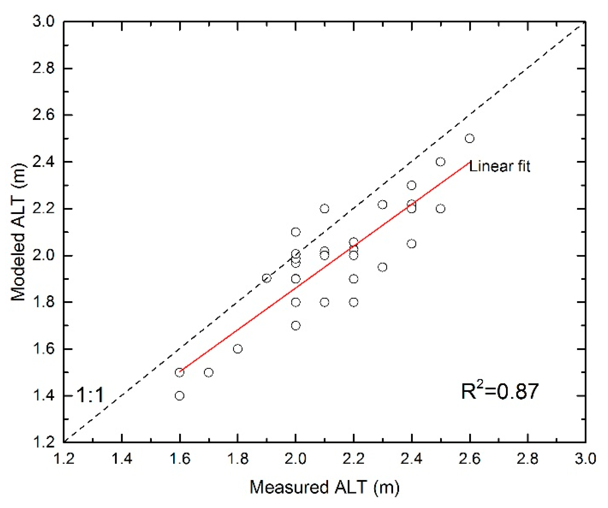
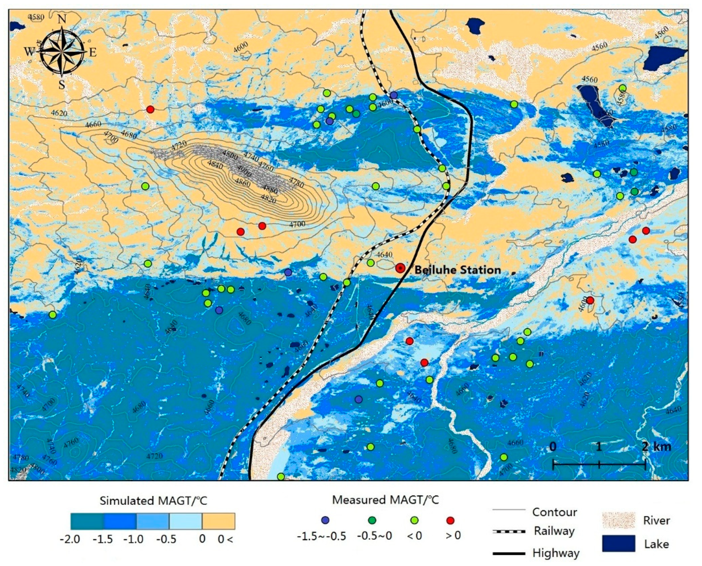
• The ecosystem types derived from high resolution satellite image provide a reliable and efficient way to scale up the ground thermal parameters and improve the resolution of the model. The GIPL 2.0 model gives a valid picture of the permafrost thermal distribution at 2.0 m spatial resolution. Present permafrost is discontinuous and occupies about 61.4% of the study region, excluding rivers and lakes. MAGT values generally range from −2.0 °C and 0 °C, but vary with ecosystem types. The modeled ALTs are highly related to the MAGT.
• The model results suggest that the permafrost area has decreased rapidly, by 26% since 1986. The mean ALT is modeled to have increased by 0.46 m. According to two climate scenarios, degradation of permafrost is suggested to occur throughout the next 60 years in most regions. A total of 8.5–35% of the area will be involved in widespread permafrost degradation. In the meantime, the average ALT will probably increase by 0.38–0.86 m.

Finally, the findings of this research contribute mainly to improving the general knowledge about permafrost thermal dynamics at a local scale for the QTP. Past, present and possible future developments of ground temperature and thaw depth have geomorphologic and geotechnical implications, which is valuable information for the government for infrastructure planning and natural hazard prediction. Additional research, in particular taking into account high-resolution satellite products on ground thermal properties and coupling with the results from the dynamic ecosystem model, is necessary to quantify possible spatial permafrost changes.

References

1. Arctic Climate Impact Assessment (ACIA). Impacts of a Warming Arctic—Arctic Climate Impact Assessment; Cambridge University Press: Cambridge, UK, 2005; p. 1042. [Google Scholar]
2. Pepin, N.; Bradley, R.; Diaz, H.; Baraër, M.; Caceres, E.; Forsythe, N.; Fowler, H.; Greenwood, G.; Hashmi, M.; Liu, X. Elevation-dependent warming in mountain regions of the world. Nate Clim. Chang. 2015, 5, 424. [Google Scholar] [CrossRef]
3. Qiu, J. The third pole. Nature 2008, 454, 24. [Google Scholar] [CrossRef] [PubMed]
4. Vaughan, D.G.; Comiso, J.C.; Allison, I.; Carrasco, J.; Kaser, G.; Kwok, R.; Mote, P.; Murray, T.; Paul, F.; Ren, J. Observations: Cryosphere. In Climate Change: The Physical Science Basis; Stocker, T.F., Qin, D., Plattner, G.K., Tignor, M., Allen, S.K., Boschung, J., Nauels, A., Xia, Y., Bex, V., Midgley, P.M., Eds.; Contribution of Working Group I to the Fifth Assessment Report of the Intergovernmental Panel on Climate Change; Cambridge University Press: Cambridge, UK; New York, NY, USA, 2013; p. 362. [Google Scholar]
5. Lawrence, D.M.; Slater, A.G.; Swenson, S.C. Simulation of present-day and future permafrost and seasonally frozen ground conditions in CCSM4. J. Clim. 2012, 25, 2207–2225. [Google Scholar] [CrossRef]
6. Kurylyk, B.L.; MacQuarrie, K.T.; McKenzie, J.M. Climate change impacts on groundwater and soil temperatures in cold and temperate regions: Implications, mathematical theory, and emerging simulation tools. Earth-Sci. Rev. 2014, 138, 313–334. [Google Scholar] [CrossRef]
7. Li, R.; Zhao, L.; Ding, Y.; Wu, T.; Xiao, Y.; Du, E.; Liu, G.; Qiao, Y. Temporal and spatial variations of the active layer along the Qinghai-Tibet Highway in a permafrost region. Sci. Bull. 2012, 57, 4609–4616. [Google Scholar] [CrossRef] [Green Version]
8. Wu, Q.; Zhang, T. Recent permafrost warming on the Qinghai-Tibetan Plateau. J. Geophys. Res. Atmos. 2008, 113, D13108. [Google Scholar] [CrossRef]
9. Wu, Q.; Zhang, T. Changes in active layer thickness over the Qinghai-Tibetan Plateau from 1995 to 2007. J. Geophys. Res. Atmos. 2010, 115, D09107. [Google Scholar] [CrossRef]
10. Wu, Q.; Zhang, T.; Liu, Y. Thermal state of the active layer and permafrost along the Qinghai-Xizang (Tibet) Railway from 2006 to 2010. Cryosphere 2012, 6, 607. [Google Scholar] [CrossRef]
11. Wu, T.; Zhao, L.; Li, R.; Wang, Q.; Xie, C.; Pang, Q. Recent ground surface warming and its effects on permafrost on the central Qinghai–Tibet Plateau. Int. J. Climatol. 2013, 33, 920–930. [Google Scholar] [CrossRef]
12. Yang, M.; Nelson, F.E.; Shiklomanov, N.I.; Guo, D.; Wan, G. Permafrost degradation and its environmental effects on the Tibetan Plateau: A review of recent research. Earth-Sci. Rev. 2010, 103, 31–44. [Google Scholar] [CrossRef]
13. Ma, W.; Niu, F.; Satoshi, A.; Dewu, J. Slope instability phenomena in permafrost regions of Qinghai-Tibet Plateau. Landslides 2006, 3, 260–264. [Google Scholar] [CrossRef]
14. Niu, F.; Yin, G.; Luo, J.; Lin, Z.; Liu, M. Permafrost Distribution along the Qinghai-Tibet Engineering Corridor, China Using High-Resolution Statistical Mapping and Modeling Integrated with Remote Sensing and GIS. Remote Sens. 2018, 10, 215. [Google Scholar] [CrossRef]
15. Qin, Y.; Wu, T.; Zhao, L.; Wu, X.; Li, R.; Xie, C.; Pang, Q.; Hu, G.; Qiao, Y.; Zhao, G.; et al. Numerical Modeling of the Active Layer Thickness and Permafrost Thermal State Across Qinghai-Tibetan Plateau. J. Geophys. Res. Atmos. 2017, 122, 604–620. [Google Scholar] [CrossRef]
16. Wu, X.; Nan, Z.; Zhao, S.; Zhao, L.; Cheng, G. Spatial modeling of permafrost distribution and properties on the Qinghai-Tibet Plateau. Permafr. Periglac. Process. 2018, 29, 86–99. [Google Scholar] [CrossRef]
17. Zou, D.; Zhao, L.; Yu, S.; Chen, J.; Hu, G.; Wu, T.; Wu, J.; Xie, C.; Wu, X.; Pang, Q. A new map of permafrost distribution on the Tibetan Plateau. Cryosphere 2017, 11, 2527. [Google Scholar] [CrossRef]
18. Ran, Y.; Li, X.; Cheng, G.; Zhang, T.; Wu, Q.; Jin, H.; Jin, R. Distribution of Permafrost in China: An Overview of Existing Permafrost Maps. Permafr. Periglac. Process. 2012, 23, 322–333. [Google Scholar] [CrossRef]
19. Jafarov, E.; Marchenko, S.; Romanovsky, V. Numerical modeling of permafrost dynamics in Alaska using a high spatial resolution dataset. Cryosphere 2012, 6, 613–624. [Google Scholar] [CrossRef] [Green Version]
20. Westermann, S.; Schuler, T.V.; Gisnas, K.; Etzelmuller, B. Transient thermal modeling of permafrost conditions in Southern Norway. Cryosphere 2013, 7, 719–739. [Google Scholar] [CrossRef] [Green Version]
21. Zhang, Y.; Wang, X.; Fraser, R.; Olthof, I.; Chen, W.; Mclennan, D.; Ponomarenko, S.; Wu, W. Modelling and mapping climate change impacts on permafrost at high spatial resolution for an Arctic region with complex terrain. Cryosphere 2013, 7, 1121–1137. [Google Scholar] [CrossRef] [Green Version]
22. Nicolsky, D.J.; Romanovsky, V.; Panda, S.; Marchenko, S.; Muskett, R. Applicability of the ecosystem type approach to model permafrost dynamics across the Alaska North Slope. J. Geophys. Res. Earth Surf. 2017, 122, 50–75. [Google Scholar] [CrossRef]
23. Ou, C.; LaRocque, A.; Leblon, B.; Zhang, Y.; Webster, K.; McLaughlin, J. Modelling and mapping permafrost at high spatial resolution using Landsat and Radarsat-2 images in Northern Ontario, Canada: Part 2—Regional mapping. Int. J. Remote Sens. 2016, 37, 2751–2779. [Google Scholar] [CrossRef]
24. Ran, Y.; Li, X.; Jin, R.; Guo, J. Remote Sensing of the Mean Annual Surface Temperature and Surface Frost Number for Mapping Permafrost in China. Arct. Antarct. Alp. Res. 2015, 47, 255–265. [Google Scholar] [CrossRef] [Green Version]
25. Westermann, S.; Peter, M.; Langer, M.; Schwamborn, G.; Schirrmeister, L.; Etzelmuller, B.; Boike, J. Transient modeling of the ground thermal conditions using satellite data in the Lena River delta, Siberia. Cryosphere 2017, 11, 1441–1463. [Google Scholar] [CrossRef] [Green Version]
26. Yin, G.; Niu, F.; Lin, Z.; Luo, J.; Liu, M. Effects of local factors and climate on permafrost conditions and distribution in Beiluhe basin, Qinghai-Tibet Plateau, China. Sci. Total Environ. 2017, 581, 472–485. [Google Scholar] [CrossRef]
27. Lin, Z.; Niu, F.; Xu, Z.; Xu, J.; Wang, P. Thermal regime of a thermokarst lake and its influence on permafrost, Beiluhe Basin, Qinghai–Tibet Plateau. Permafr. Periglac. Process. 2010, 21, 315–324. [Google Scholar] [CrossRef]
28. Luo, J.; Niu, F.; Lin, Z.; Liu, M.; Yin, G. Thermokarst lake changes between 1969 and 2010 in the beilu river basin, qinghai–tibet plateau, China. Sci. Bull. 2015, 60, 556–564. [Google Scholar] [CrossRef]
29. Yun, H.; Wu, Q.; Zhuang, Q.; Chen, A.; Yu, T.; Lyu, Z.; Yang, Y.; Jin, H.; Liu, G.; Qu, Y.; et al. Consumption of atmospheric methane by the Qinghai–Tibet Plateau alpine steppe ecosystem. Cryosphere 2018, 12, 16. [Google Scholar] [CrossRef]
30. Wu, Q.; Hou, Y.; Yun, H.; Liu, Y. Changes in active-layer thickness and near-surface permafrost between 2002 and 2012 in alpine ecosystems, Qinghai–Xizang (Tibet) Plateau, China. Glob. Planet. Chang. 2015, 124, 149–155. [Google Scholar] [CrossRef]
31. Tipenko, G.; Marchenko, S.; Romanovsky, V.; Groshev, V.; Sazonova, T. Spatially Distributed Model of Permafrost Dynamics in Alaska. In Proceedings of the AGU Fall Meeting, San Francisco, CA, USA, 13–17 December 2004. [Google Scholar]
32. Wu, Q.; Zhang, T.; Liu, Y. Permafrost temperatures and thickness on the Qinghai-Tibet Plateau. Glob. Planet. Chang. 2010, 72, 32–38. [Google Scholar] [CrossRef]
33. Westermann, S.; Elberling, B.; Højlund Pedersen, S.; Stendel, M.; Hansen, B.U.; Liston, G.E. Future permafrost conditions along environmental gradients in Zackenberg, Greenland. Cryosphere 2015, 9, 719–735. [Google Scholar] [CrossRef] [Green Version]
34. Hipp, T.; Etzelmüller, B.; Farbrot, H.; Schuler, T.; Westermann, S. Modelling borehole temperatures in Southern Norway–insights into permafrost dynamics during the 20th and 21st century. Cryosphere 2012, 6, 553–571. [Google Scholar] [CrossRef]
35. Rogelj, J.; den Elzen, M.; Höhne, N.; Fransen, T.; Fekete, H.; Winkler, H.; Schaeffer, R.; Sha, F.; Riahi, K.; Meinshausen, M. Paris Agreement climate proposals need a boost to keep warming well below 2 °C. Nature 2016, 534, 631. [Google Scholar] [CrossRef]
36. UNFCCC. Adoption of the Paris Agreement; Report No. FCCC/CP/2015/L.9/Rev.1; United Nations: New York, NY, USA, 2015; Available online: http://unfccc.int/resource/docs/2015/cop21/eng/l09r01.pdf (accessed on 29 January 2016).
37. Gisnas, K.; Etzelmuller, B.; Farbrot, H.; Schuler, T.V.; Westermann, S. CryoGRID 1.0: Permafrost Distribution in Norway estimated by a Spatial Numerical Model. Permafr. Periglac. Process. 2013, 24, 2–19. [Google Scholar] [CrossRef] [Green Version]
38. Lin, Z.; Burn, C.; Niu, F.; Luo, J.; Liu, M.; Yin, G. The thermal regime, including a reversed thermal offset, of arid permafrost sites with variations in vegetation cover density, Wudaoliang Basin, Qinghai-Tibet Plateau. Permafr. Periglac. Process. 2015, 26, 142–159. [Google Scholar] [CrossRef]
39. Gubler, S.; Endrizzi, S.; Gruber, S.; Purves, R.S. Sensitivities and uncertainties of modeled ground temperatures in mountain environments. Geosci. Model Dev. 2013, 6, 1319–1336. [Google Scholar] [CrossRef] [Green Version]
40. Langer, M.; Westermann, S.; Heikenfeld, M.; Dorn, W.; Boike, J. Satellite-based modeling of permafrost temperatures in a tundra lowland landscape. Remote Sens. Environ. 2013, 135, 12–24. [Google Scholar] [CrossRef] [Green Version]
41. Nicolsky, D.J.; Romanovsky, V.E. Modeling Long-Term Permafrost Degradation. J. Geophys. Res. Earth Surf. 2018, 123, 1756–1771. [Google Scholar] [CrossRef]
42. Kurylyk, B.L.; Hayashi, M.; Quinton, W.L.; Mckenzie, J.M.; Voss, C.I. Influence of vertical and lateral heat transfer on permafrost thaw, peatland landscape transition, and groundwater flow. Water Resour. Res. 2016, 52, 1286–1305. [Google Scholar] [CrossRef] [Green Version]
43. Christensen, T.R.; Johansson, T.; Åkerman, H.J.; Mastepanov, M.; Malmer, N.; Friborg, T.; Crill, P.; Svensson, B.H. Thawing sub-arctic permafrost: Effects on vegetation and methane emissions. Geophys. Res. Lett. 2004, 31. [Google Scholar] [CrossRef]
44. Jorgenson, M.T.; Racine, C.H.; Walters, J.C.; Osterkamp, T.E. Permafrost Degradation and Ecological Changes Associated with a Warming Climate in Central Alaska. Clim. Chang. 2001, 48, 551–579. [Google Scholar] [CrossRef]
45. Jorgenson, M.T.; Harden, J.; Kanevskiy, M.; O’Donnell, J.; Wickland, K.; Ewing, S.; Manies, K.; Zhuang, Q.; Shur, Y.; Striegl, R.; et al. Reorganization of vegetation, hydrology and soil carbon after permafrost degradation across heterogeneous boreal landscapes. Environ. Res. Lett. 2013, 8, 035017. [Google Scholar] [CrossRef]
46. Wu, Q.; Zhang, Z.; Gao, S.; Ma, W. Thermal impacts of engineering activities and vegetation layer on permafrostin different alpine ecosystems of the Qinghai—Tibet Plateau, China. Cryosphere 2016, 10, 1695–1706. [Google Scholar] [CrossRef]
47. Nicolsky, D.J.; Romanovsky, V.E.; Tipenko, G.S. Estimation of thermal properties of saturated soils using in-situ temperature measurements. Cryosphere 2007, 1, 213–269. [Google Scholar] [CrossRef]
48. Jin, H.; Chang, X.; Wang, S. Evolution of permafrost on the Qinghai-Xizang (Tibet) Plateau since the end of the late Pleistocene. J. Geophys. Res. Earth Surf. 2007, 112, F02S09. [Google Scholar] [CrossRef]
49. Peng, H.; Ma, W.; Mu, Y.H.; Jin, L. Impact of permafrost degradation on embankment deformation of Qinghai-Tibet Highway in permafrost regions. J. Cent. South Univ. 2015, 22, 1079–1086. [Google Scholar] [CrossRef]
Figure 1. The location of the study area: (a) The Beiluhe basin in the central Qinghai-Tibet Plateau (QTP); (b) Gao fen-1 satellite image (2.0 m resolution) of the study area and the locations of the climate station and the validation sites.
Remotesensing 11 01294 g001
Figure 2. Summer mean nt factor vs. Normalized Differential Vegetation Index (NDVI) based on in situ measurements (2012–2016) [25]. The red line represents the fit following Equation (2).
Remotesensing 11 01294 g002
Figure 3. Scatterplot of the simulated and measured daily ground surface temperature for multiple field sites. Each graph includes one site with a land cover type.
Remotesensing 11 01294 g003
Figure 4. Scatterplot of the simulated and measured active-layer thicknesses (ALT) in different geomorphological units.
Remotesensing 11 01294 g004
Figure 5. Modeled permafrost thermal condition (MAGT at 10 m depth) for the period of 2006–2015.
Remotesensing 11 01294 g005
Figure 6. Modeled mean active-layer thickness for the period of 2006–2015.
Remotesensing 11 01294 g006
Figure 7. Modeled evolution of the ground temperatures at 10 m for different periods. (a) 1986–1995, (b) 1996–2005, (c,d) 2016–2045 for the low- and high-rate runs, (e,f) 2046–2075 for the low (0.015 °C yr−1) and high (0.065 °C yr−1) climate warming trends.
Remotesensing 11 01294 g007
Figure 8. Statistics of modeled ground temperature distribution. (a) MAGTs at 10 m depth for different temperature ranges; (b) permafrost area evolution.
Remotesensing 11 01294 g008
Figure 9. Modeled evolution of the active-layer thickness. (a) 1986–1995, (b) 1996–2005, (c,d) 2016–2045 for the low- and high-rate runs, (e,f) 2046–2075 for the low- and high-rate runs.
Remotesensing 11 01294 g009
Figure 10. Distributions of modeled ALTs for different ecosystem units in 1986–1995, 1996–2005, 2006–2015, 2016–2045, and 2046–2075.
Remotesensing 11 01294 g010