A New RGB-D SLAM Method with Moving Object Detection for Dynamic Indoor Scenes

Abstract
1. Introduction
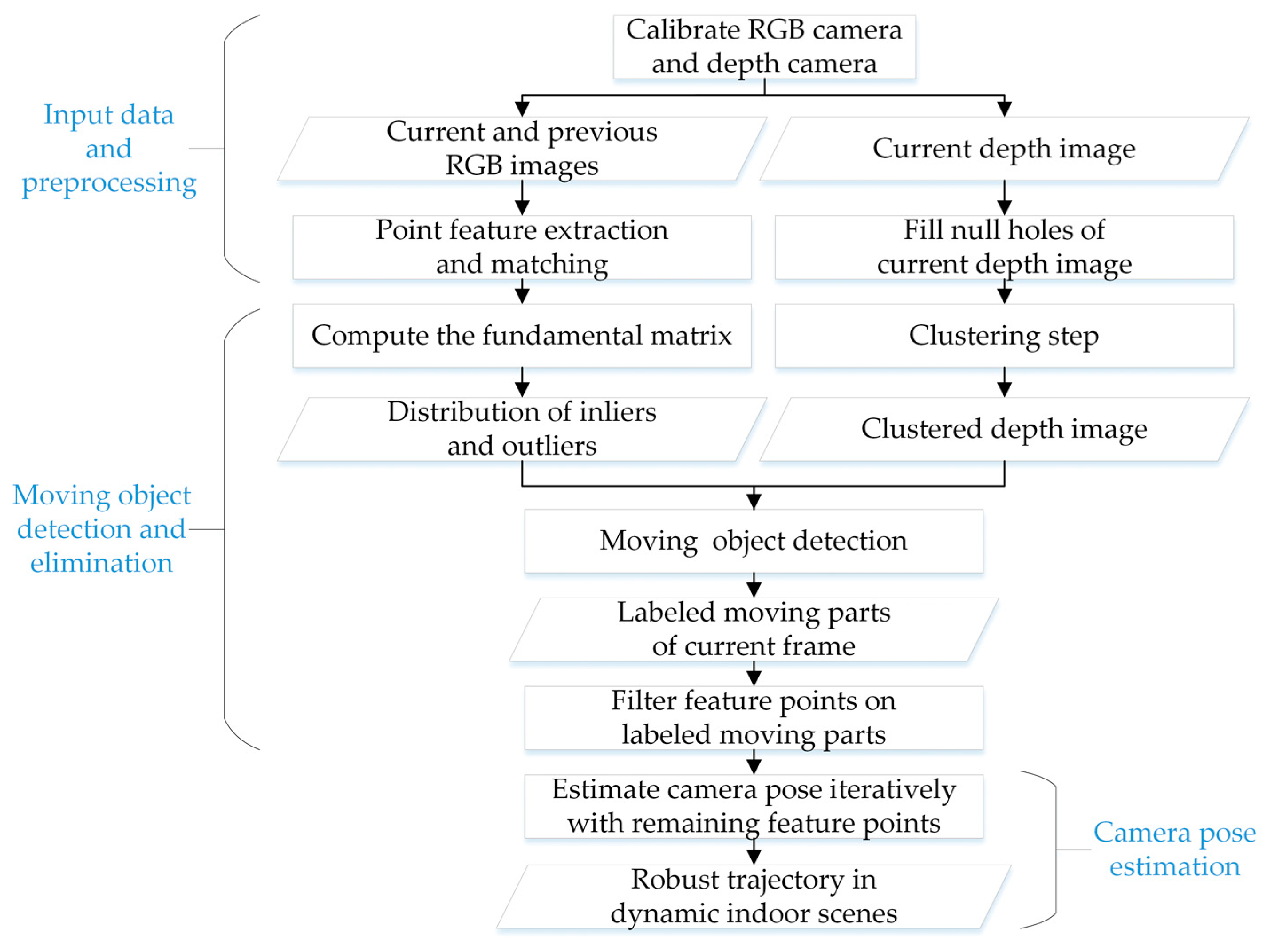
2. Methodology
2.1. Input Data and Preprocessing
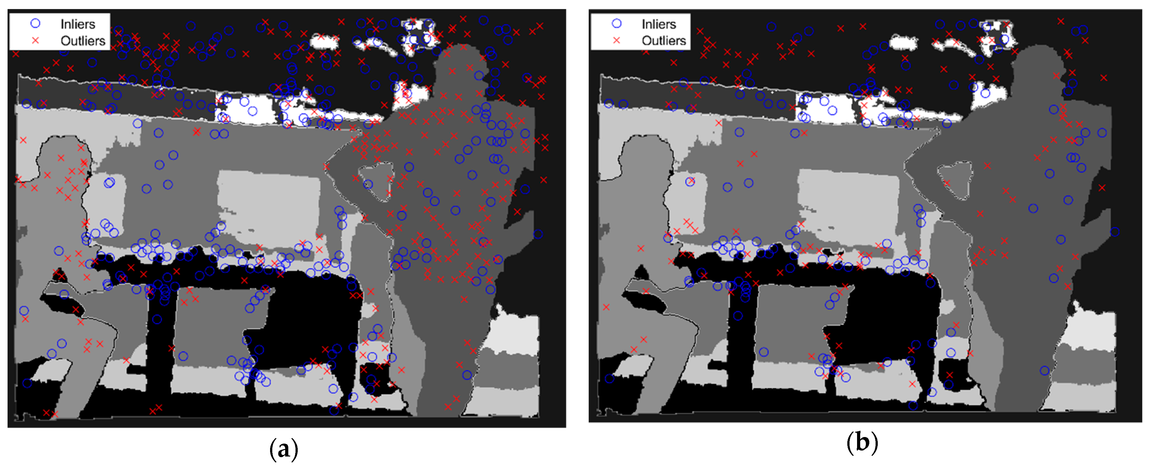
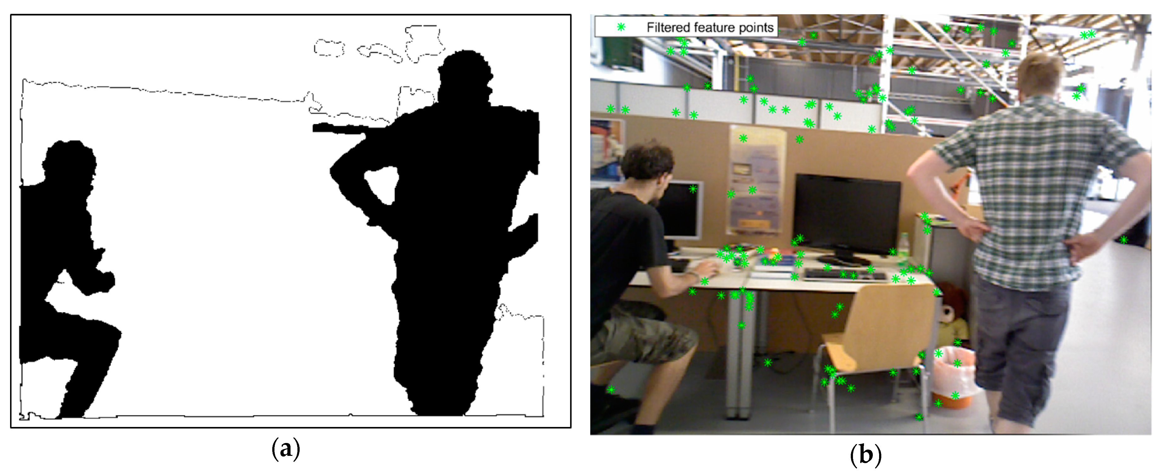
2.2. Moving Object Detection and Elimination
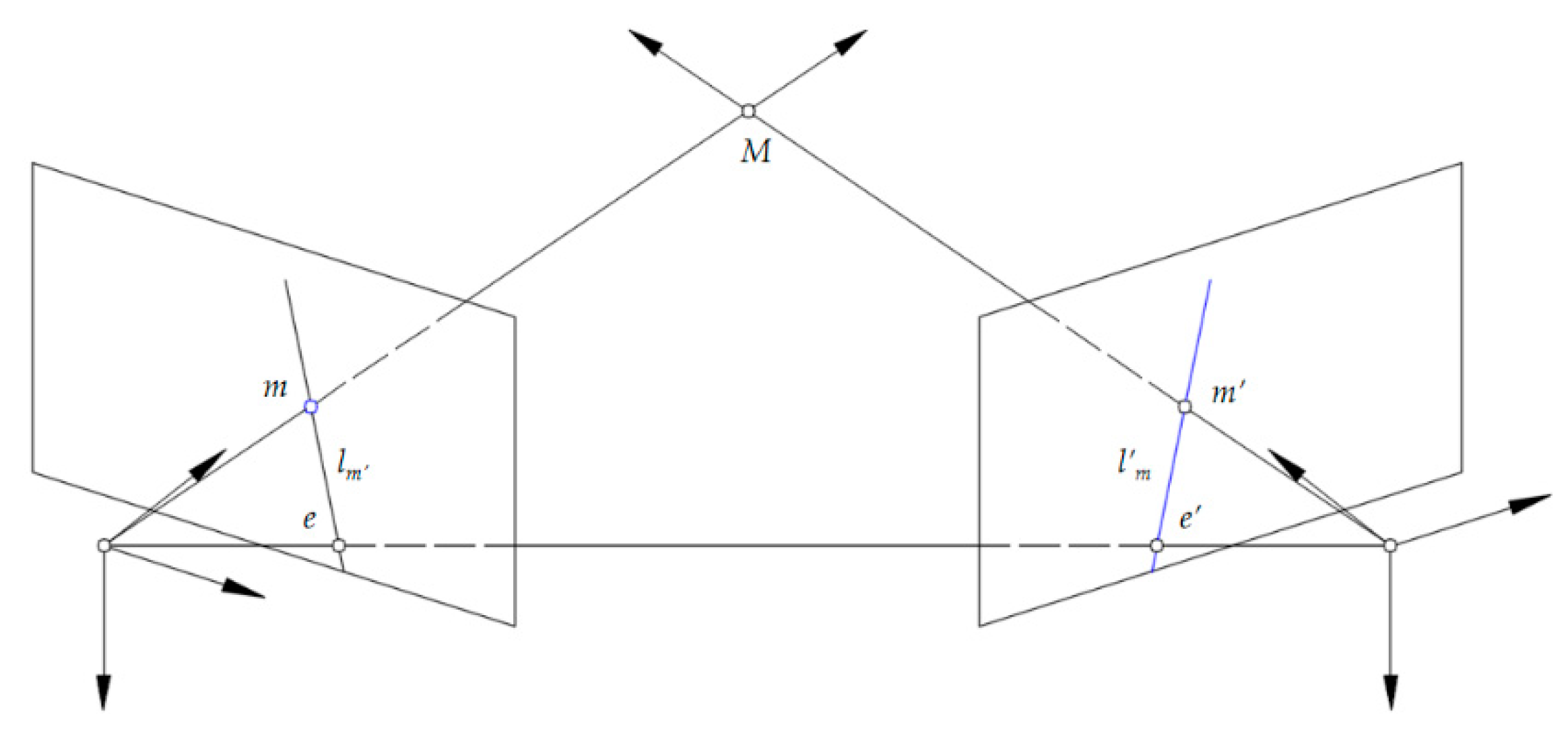
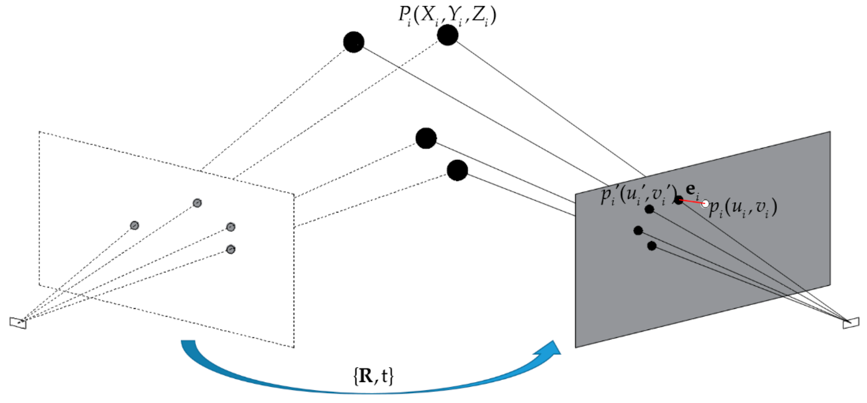
2.3. Camera Pose Estimation
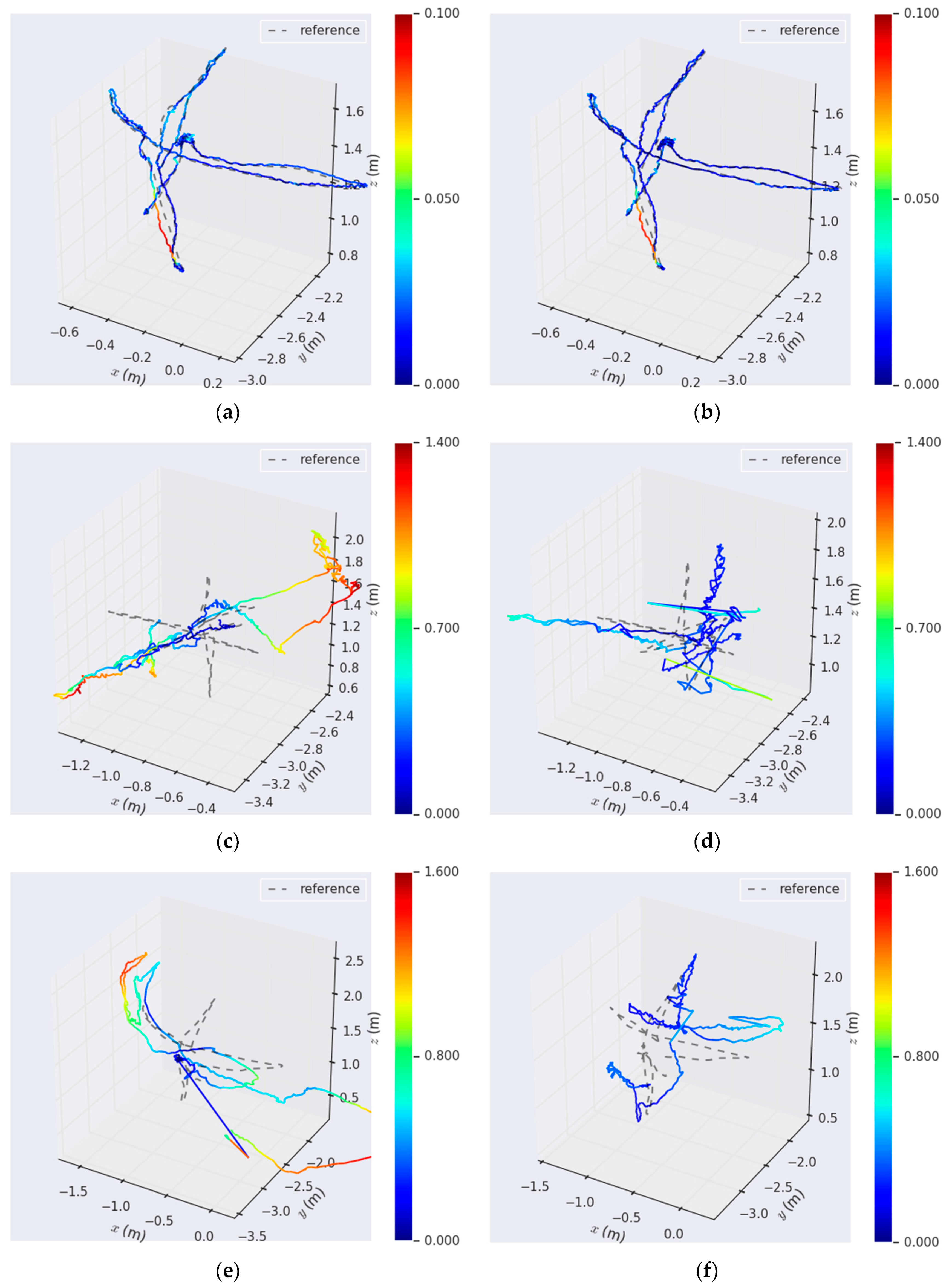
3. Experimental Results
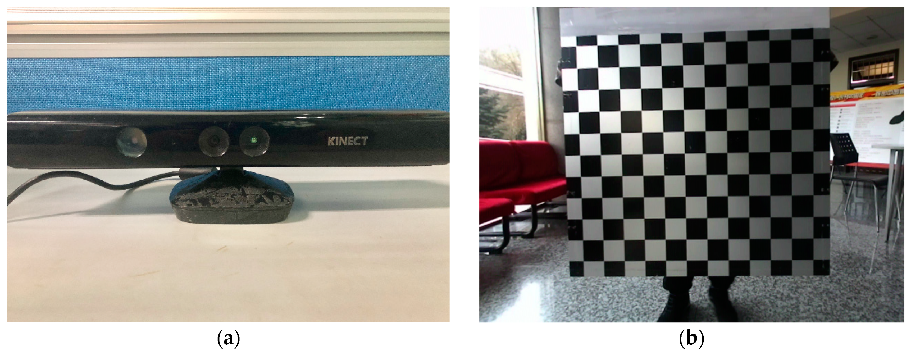
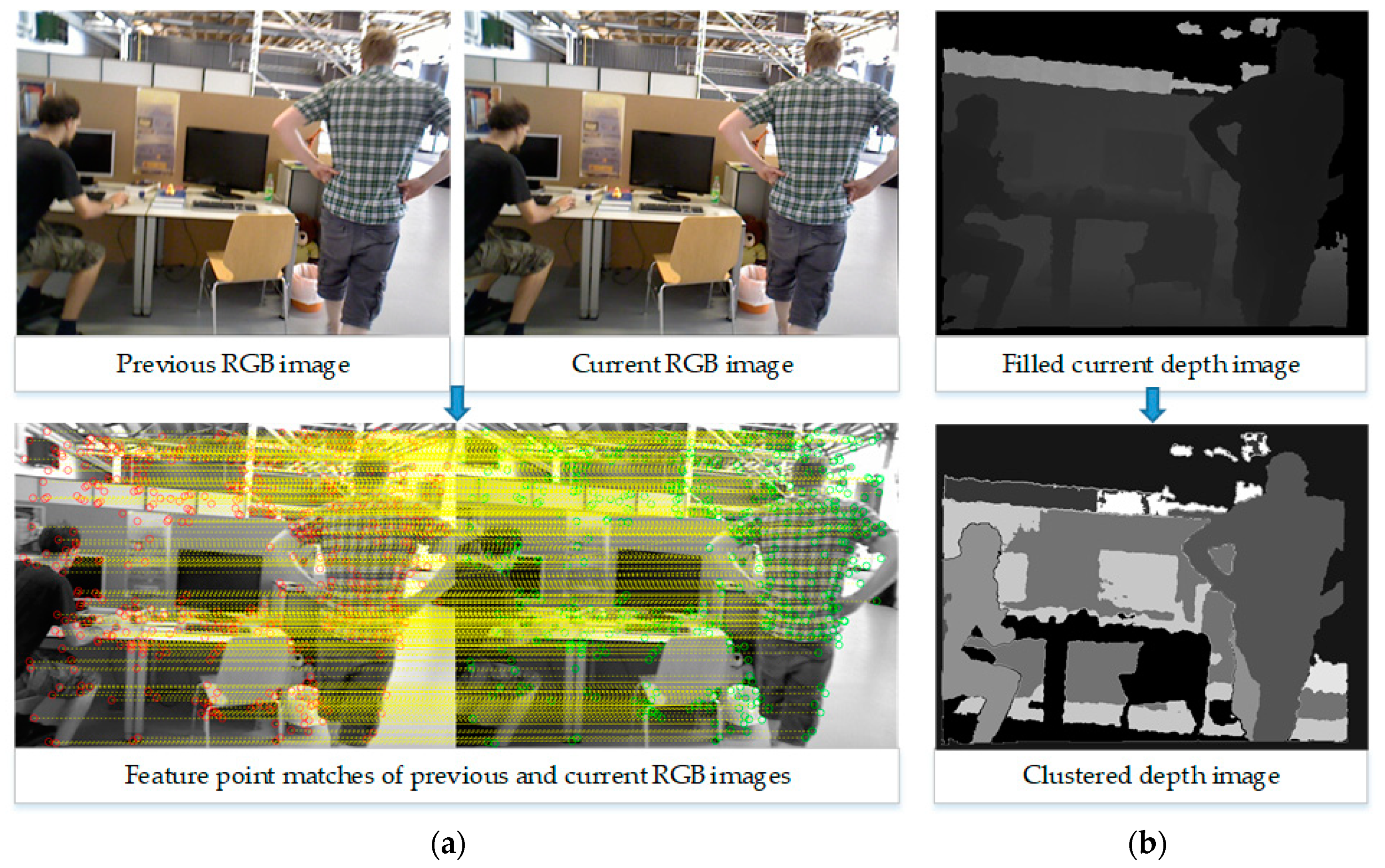
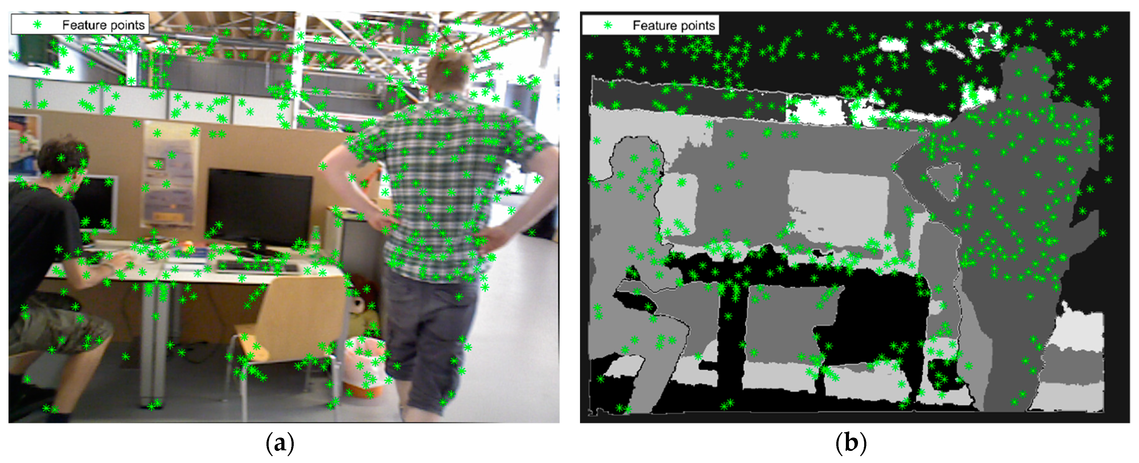
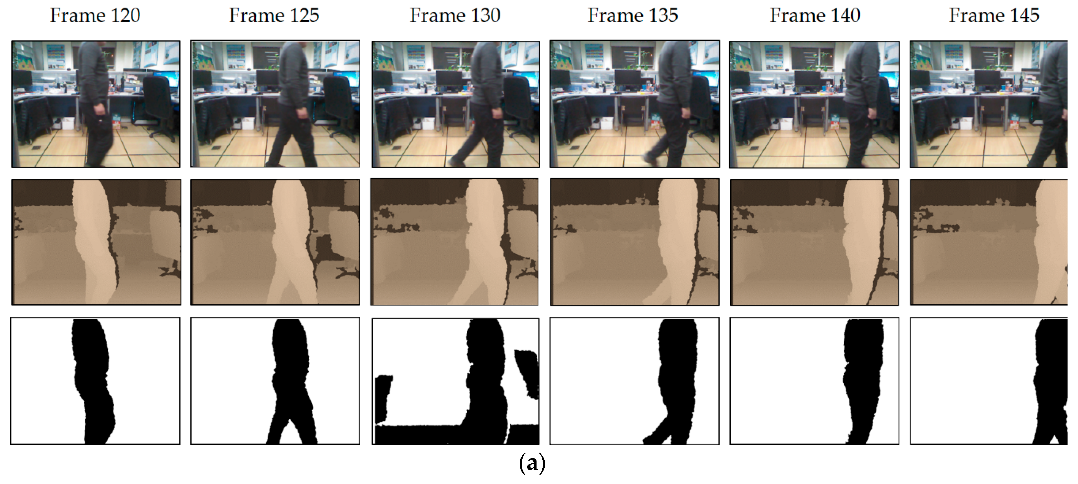
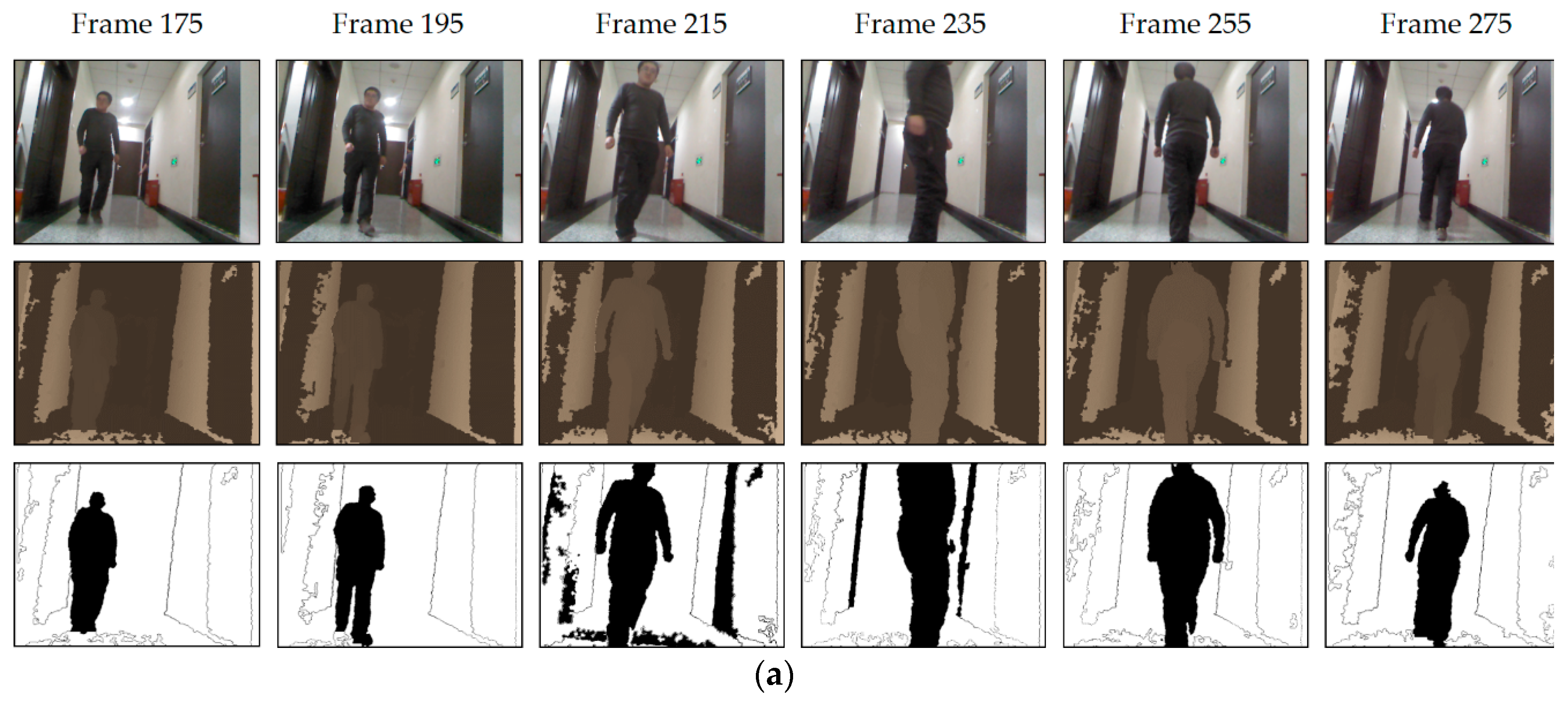
3.1. Testing with Sequence Images Captured by Our RGB-D Camera
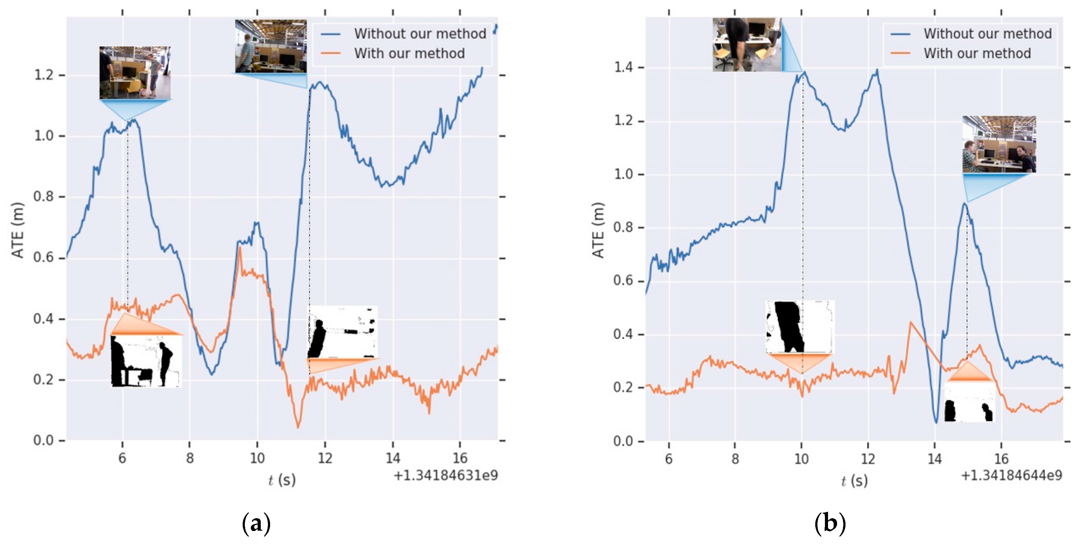
3.2. Evaluation Using TUM RGB-D SLAM Datasets
4. Conclusions
Author Contributions
Funding
Acknowledgments
Conflicts of Interest
Abbreviations
| SLAM | Simultaneous localization and mapping |
| LiDAR | Light detection and ranging |
| GPS | Global positioning system |
| IMUs | Inertial measurement units |
| 3D | Three-dimension |
| SURF | Speeded-Up Robust Features |
| ORB | Oriented FAST and rotated BRIEF |
| ORB-SLAM | ORB feature based SLAM |
| DoFs | Degree of freedom |
| DVO | Dense visual odometry |
| RFS | Random finite set |
| FOV | Field of view |
| BaMVO | Background model-based dense-visual-odometry |
| IAICP | Intensity assisted iterative closest point |
| FPS | Frames per second |
| EPnP | Efficient perspective-n-point method |
| BA | Bundle adjustment |
| ATE | Absolute trajectory error |
| RMSE | Root mean square error |
| RPE | Relative pose error |
References
- Durrant-Whyte, H.; Bailey, T. Simultaneous localization and mapping: Part I. IEEE Robot. Autom. Mag. 2006, 13, 99–110. [Google Scholar] [CrossRef]
- Bailey, T.; Durrant-Whyte, H. Simultaneous localization and mapping (SLAM): Part II. IEEE Robot. Autom. Mag. 2006, 13, 108–117. [Google Scholar] [CrossRef]
- Dissanayake, M.W.M.G.; Newman, P.; Clark, S.; Durrant-Whyte, H.F.; Csorba, M.A. Solution to the simultaneous localization and map building (SLAM) problem. IEEE Trans. Robot. Autom. 2001, 17, 229–241. [Google Scholar] [CrossRef]
- Hess, W.; Kohler, D.; Rapp, H.; Andor, D. Real-time loop closure in 2D LIDAR SLAM. In Proceedings of the IEEE International Conference on Robotics and Automation, Stockholm, Sweden, 16–21 May 2016; pp. 1271–1278. [Google Scholar] [CrossRef]
- Fuentes-Pacheco, J.; Ruiz-Ascencio, J.; Rendón-Mancha, J.M. Visual simultaneous localization and mapping: A survey. Artif. Intell. Rev. 2015, 43, 55–81. [Google Scholar] [CrossRef]
- Ido, J.; Shimizu, Y.; Matsumoto, Y.; Ogasawara, T. Indoor Navigation for a Humanoid Robot Using a View Sequence. Int. J. Robot. Res. 2009, 28, 315–325. [Google Scholar] [CrossRef]
- Celik, K.; Chung, S.J.; Clausman, M.; Somani, A.K. Monocular vision SLAM for indoor aerial vehicles. In Proceedings of the 2009 IEEE/RSJ International Conference on Intelligent Robots and Systems (ICRA), St. Louis, MO, USA, 11–15 October 2009; pp. 1566–1573. [Google Scholar]
- Davison, A.J.; Reid, I.D.; Molton, N.D.; Stasse, O. MonoSLAM: Real-time single camera SLAM. IEEE Trans. Pattern Anal. Mach. Intell. 2007, 29, 1052–1067. [Google Scholar] [CrossRef] [PubMed]
- Lemaire, T.; Lacroix, S. Monocular-vision based SLAM using Line Segments. In Proceedings of the IEEE International Conference on Robotics and Automation (ICRA), Roma, Italy, 10–14 April 2007; pp. 2791–2796. [Google Scholar]
- Celik, K.; Chung, S.J.; Somani, A. Mono-vision corner SLAM for indoor navigation. In Proceedings of the 2008 IEEE International Conference on Electro/information Technology, Winsor, ON, Canada, 7–9 June 2008; pp. 343–348. [Google Scholar]
- Wu, K.; Di, K.; Sun, X.; Wan, W.; Liu, Z. Enhanced monocular visual odometry integrated with laser distance meter for astronaut navigation. Sensors 2014, 14, 4981–5003. [Google Scholar] [CrossRef]
- Jiang, Y.; Chen, H.; Xiong, G.; Scaramuzza, D. ICP Stereo Visual Odometry for Wheeled Vehicles based on a 1DOF Motion Prior. In Proceedings of the 2014 IEEE International Conference on Robotics and Automation (ICRA), Hong Kong, China, 31 May–7 June 2014; pp. 585–592. [Google Scholar]
- Gomez-Ojeda, R.; Gonzalez-Jimenez, J. Robust stereo visual odometry through a probabilistic combination of points and line segments. In Proceedings of the 2016 IEEE International Conference on Robotics and Automation (ICRA), Stockholm, Sweden, 16–21 May 2016; pp. 2521–2526. [Google Scholar]
- Gomez-Ojeda, R.; Moreno, F.A.; Scaramuzza, D.; Gonzalez-Jimenez, J. PL-SLAM: A Stereo SLAM System through the Combination of Points and Line Segments. arXiv 2017, arXiv:1705.09479. [Google Scholar] [CrossRef]
- Kaess, M.; Dellaert, F. Probabilistic structure matching for visual SLAM with a multi-camera rig. Comput. Vis. Image Underst. 2010, 114, 286–296. [Google Scholar] [CrossRef]
- Moratuwage, D.; Wang, D.; Rao, A.; Senarathne, N. RFS Collaborative Multivehicle SLAM: SLAM in Dynamic High-Clutter Environments. IEEE Robot. Autom. Mag. 2014, 21, 53–59. [Google Scholar] [CrossRef]
- He, Y.; Zhao, J.; Guo, Y.; He, W.; Yuan, K. PL-VIO: Tightly-Coupled Monocular Visual-Inertial Odometry Using Point and Line Features. Sensors 2018, 18, 1159. [Google Scholar] [CrossRef] [PubMed]
- Bay, H.; Ess, A.; Tuytelaars, T.; Gool, L.V. Speeded-Up Robust Features (SURF). Comput. Vis. Image Underst. 2008, 110, 346–359. [Google Scholar] [CrossRef]
- Rublee, E.; Rabaud, V.; Konolige, K. ORB: An efficient alternative to SIFT or SURF. In Proceedings of the 2011 IEEE International Conference on Computer Vision (ICCV), Barcelona, Spain, 6–13 November 2011; pp. 2564–2571. [Google Scholar]
- Hu, G.; Huang, S.; Zhao, L.; Alempijevic, A.; Dissanayake, G. A robust RGB-D SLAM algorithm. In Proceedings of the 2012 IEEE/RSJ International Conference on Intelligent Robots and Systems (IROS), Vilamoura, Portugal, 7–12 October 2012; pp. 1714–1719. [Google Scholar]
- Ji, Y.; Yamashita, A.; Asama, H. RGB-D SLAM using vanishing point and door plate information in corridor environment. Intell. Serv. Robot. 2015, 8, 105–114. [Google Scholar] [CrossRef]
- Mur-Artal, R.; Tardós, J.D. ORB-SLAM2: An Open-Source SLAM System for Monocular, Stereo, and RGB-D Cameras. IEEE Trans. Robot. 2017, 33, 1255–1262. [Google Scholar] [CrossRef]
- Kerl, C.; Sturm, J.; Cremers, D. Dense visual SLAM for RGB-D cameras. In Proceedings of the 2013 IEEE/RSJ International Conference on Intelligent Robots and Systems, Tokyo, Japan, 3–7 November 2013; pp. 2100–2106. [Google Scholar]
- Wang, C.C.; Thorpe, C.; Thrun, S.; Hebert, M.; Durrant-Whyte, H. Simultaneous Localization, Mapping and Moving Object Tracking. Inter. J. Robot. Res. 2007, 26, 889–916. [Google Scholar] [CrossRef]
- Alcantarilla, P.; Yebes, J.; Almazn, j.; Bergasa, L. On combining visual SLAM and dense scene flow to increase the robustness of localization and mapping in dynamic environments. In Proceedings of the 2012 IEEE International Conference on Robotics and Automation (ICRA), Saint Paul, MN, USA, 14–18 May 2012; pp. 1290–1297. [Google Scholar]
- Wang, Y.; Huang, S. Towards dense moving object segmentation based robust dense RGB-D SLAM in dynamic scenarios. In Proceedings of the 2014 13th International Conference on Control Automation Robotics& Vision (ICARCV), Singapore, 10–12 December 2014; pp. 1841–1846. [Google Scholar]
- Bakkay, M.C.; Arafa, M.; Zagrouba, E. Dense 3D SLAM in dynamic scenes using Kinect. In Proceedings of the 7th Iberian Conference on Pattern Recognition and Image Analysis, Santiago de Compostela, Spain, 17–19 June 2015; pp. 121–129. [Google Scholar]
- Sun, Y.; Liu, M.; Meng, Q.H. Improving RGB-D SLAM in dynamic environments: A motion removal approach. Robot. Autom. Syst. 2017, 89, 110–122. [Google Scholar] [CrossRef]
- Sturm, J.; Engelhard, N.; Endres, F.; Burgard, W.; Cremers, D. A benchmark for the evaluation of RGB-D SLAM systems. In Proceedings of the 2012 IEEE/RSJ International Conference on Intelligent Robots and Systems (IROS), Algarve, Portugal, 7–12 October 2012; pp. 573–580. [Google Scholar]
- Yang, S.; Wang, J.; Wang, G.; Hu, X.; Zhou, M.; Liao, Q. Robust RGB-D SLAM in dynamic environment using faster R-CNN. In Proceedings of the 2017 3rd IEEE International Conference on Computer and Communications (ICCC), Chengdu, China, 13–16 December 2017; pp. 5702–5708. [Google Scholar]
- Ren, S.; He, K.; Girshick, R.; Sun, J. Faster r-cnn: Towards real-time object detection withregion proposal networks. IEEE Trans. Pattern Anal. Mach. Intell. 2017, 39, 1137–1142. [Google Scholar] [CrossRef]
- Zhong, F.; Wang, S.; Zhang, Z.; Zhou, C.; Wang, Y. Detect-SLAM: Making Object Detection and SLAM Mutually Beneficial. In Proceedings of the 2018 IEEE Winter Conference on Applications of Computer Vision, Lake Tahoe, NV, USA, 12–15 March 2018; pp. 1001–1010. [Google Scholar]
- Yang, D.; Bi, S.; Wang, W.; Yuan, C.; Wang, W.; Qi, X.; Cai, Y. DRE-SLAM: Dynamic RGB-D Encoder SLAM for a Differential-Drive Robot. Remote Sens. 2019, 11, 380. [Google Scholar] [CrossRef]
- Redmon, J.; Farhadi, A. Yolov3: An incremental improvement. arXiv 2018, arXiv:1804.02767. [Google Scholar]
- Moratuwage, D.; Vo, B.-N.; Wang, D. Collaborative multi-vehicle SLAM with moving object tracking. In Proceedings of the 2013 IEEE Int. Conf. Robotics &Automation (ICRA), Karlsruhe, Germany, 6–10 May 2013; pp. 5702–5708. [Google Scholar]
- Zou, D.; Tan, P. CoSLAM: collaborative visual SLAM in dynamic environments. IEEE Trans. Pattern Anal. Mach. Intell. 2013, 35, 354–366. [Google Scholar] [CrossRef]
- Kerl, C.; Sturm, J.; Cremers, D. Robust odometry estimation for RGB-D cameras. In Proceedings of the 2013 IEEE Int. Conf. Robotics &Automation (ICRA), Karlsruhe, Germany, 6–10 May 2013; pp. 3748–3754. [Google Scholar]
- Lee, D.; Myung, H. Solution to the SLAM Problem in Low Dynamic Environments Using a Pose Graph and an RGB-D Sensor. Sensors 2014, 14, 12467–12496. [Google Scholar] [CrossRef]
- Kim, D.H.; Kim, J.H. Effective Background Model-Based RGB-D Dense Visual Odometry in a Dynamic Environment. IEEE Trans. Robot. 2017, 32, 1565–1573. [Google Scholar] [CrossRef]
- Li, S.; Lee, D. RGB-D SLAM in Dynamic Environments using Static Point Weighting. IEEE Robot. Autom. Lett. 2017, 2, 2263–2270. [Google Scholar] [CrossRef]
- Zhang, Z. A flexible new technique for camera calibration. IEEE Trans. Pattern Anal. Mach. Intell. 2000, 22, 1330–1334. [Google Scholar] [CrossRef]
- Soille, P. Morphological Image Analysis: Principles and Applications. Sens. Rev. 1999, 28, 800–801. [Google Scholar]
- Richard, H.; Andrew, Z. Multiple View Geometry in Computer Vision, 2nd ed.; Cambridge University Press: Cambridge, UK, 2003; pp. 241–253. [Google Scholar]
- Massart, D.L.; Kaufman, L. Least median of squares: a robust method for outlier and model error detection in regression and calibration. Analytica Chimica Acta 1986, 187, 171–179. [Google Scholar] [CrossRef]
- Lepetit, V.; Moreno-Noguer, F.; Fua, P. EPnP: An accurate O(n) solution to the PnP problem. Inter. J. Comput. Vis. 2009, 81, 155–166. [Google Scholar] [CrossRef]
- Hall, B.C. Lie Groups, Lie Algebras, and Representations, 2nd ed.; Springer: New York, NY, USA, 2015; pp. 49–75. [Google Scholar]
- Kümmerle, R.; Grisetti, G.; Strasdat, H.; Konolige, K.; Burgard, W. G2o: A general framework for graph optimization. In Proceedings of the 2011 IEEE International Conference on Robotics and Automation (ICRA), Shanghai, China, 9–13 May 2011; pp. 3607–3613. [Google Scholar]


| Camera | |||||||||
|---|---|---|---|---|---|---|---|---|---|
| RGB | 584.35 | 584.33 | 317.97 | 252.80 | −0.10585 | 0.27096 | 0.0 | 0.00504 | −0.00166 |
| Depth | 519.95 | 519.55 | 315.82 | 238.71 | 0.04810 | −0.19281 | 0.0 | 0.00458 | −0.00014 |
| Rotation Angles (°) | −0.00079 | −0.00084 | −0.00541 |
| Translation Vector (mm) | −25.59983 | 0.16700 | −0.40571 |
| Dynamic TUM RGB-D Datasets | Without Moving Object Detection ATE (m) | With Moving Object Detection ATE (m) | ||||||
|---|---|---|---|---|---|---|---|---|
| Max. | Avg. | Min. | RMSE | Max. | Avg. | Min. | RMSE | |
| fr3/sitting_static | 0.0381 | 0.0078 | 0.0007 | 0.0087 | 0.0255 | 0.0059 | 0.0002 | 0.0066 |
| fr3/sitting_halfsphere | 0.0971 | 0.0194 | 0.0018 | 0.0230 | 0.0919 | 0.0152 | 0.0017 | 0.0196 |
| fr3/walking_static | 0.6391 | 0.3513 | 0.0587 | 0.3843 | 0.6161 | 0.2691 | 0.0231 | 0.3080 |
| fr3/walking_xyz | 1.3661 | 0.6309 | 0.0612 | 0.7328 | 0.8196 | 0.2768 | 0.0430 | 0.3047 |
| fr3/walking_halfsphere | 1.5683 | 0.5831 | 0.0690 | 0.6891 | 0.6246 | 0.2972 | 0.1088 | 0.3116 |
| fr3/walking_rpy | 1.1136 | 0.4975 | 0.1118 | 0.5523 | 0.9351 | 0.4637 | 0.0708 | 0.4983 |
| TUM RGB-D Datasets Category: Dynamic Objects | Translation RMSE (m/s) | Rotation RMSE (°/s) | |||||
|---|---|---|---|---|---|---|---|
| DVO | BaMVO | Ours | DVO | BaMVO | Ours | ||
| Low Dynamic Environment | fr2/desk_with_person | 0.0354 | 0.0352 | 0.0069 | 1.5368 | 1.2159 | 0.4380 |
| fr3/sitting_static | 0.0157 | 0.0248 | 0.0077 | 0.6084 | 0.6977 | 0.2595 | |
| fr3/sitting_xyz | 0.0453 | 0.0482 | 0.0117 | 1.4980 | 1.3885 | 0.4997 | |
| fr3/sitting_halfsphere | 0.1005 | 0.0589 | 0.0245 | 4.6490 | 2.8804 | 0.5643 | |
| fr3/sitting_rpy | 0.1735 | 0.1872 | 0.0234 | 6.0164 | 5.9834 | 0.7838 | |
| High Dynamic Environment | fr3/walking_static | 0.3818 | 0.1339 | 0.1881 | 6.3502 | 2.0833 | 3.2101 |
| fr3/walking_xyz | 0.4360 | 0.2326 | 0.2158 | 7.6669 | 4.3911 | 3.6476 | |
| fr3/walking_halfsphere | 0.2628 | 0.1738 | 0.1908 | 5.2179 | 4.2863 | 3.3321 | |
| fr3/walking_rpy | 0.4038 | 0.3584 | 0.3270 | 7.0662 | 6.3398 | 6.3215 | |
© 2019 by the authors. Licensee MDPI, Basel, Switzerland. This article is an open access article distributed under the terms and conditions of the Creative Commons Attribution (CC BY) license (http://creativecommons.org/licenses/by/4.0/).
Share and Cite
Wang, R.; Wan, W.; Wang, Y.; Di, K. A New RGB-D SLAM Method with Moving Object Detection for Dynamic Indoor Scenes. Remote Sens. 2019, 11, 1143. https://doi.org/10.3390/rs11101143
Wang R, Wan W, Wang Y, Di K. A New RGB-D SLAM Method with Moving Object Detection for Dynamic Indoor Scenes. Remote Sensing. 2019; 11(10):1143. https://doi.org/10.3390/rs11101143
Chicago/Turabian StyleWang, Runzhi, Wenhui Wan, Yongkang Wang, and Kaichang Di. 2019. "A New RGB-D SLAM Method with Moving Object Detection for Dynamic Indoor Scenes" Remote Sensing 11, no. 10: 1143. https://doi.org/10.3390/rs11101143
APA StyleWang, R., Wan, W., Wang, Y., & Di, K. (2019). A New RGB-D SLAM Method with Moving Object Detection for Dynamic Indoor Scenes. Remote Sensing, 11(10), 1143. https://doi.org/10.3390/rs11101143