Article

Radiometric Calibration of UAV Remote Sensing Image with Spectral Angle Constraint

1
School of Remote Sensing and Information Engineering, Wuhan University, Wuhan 430079, China
2
China Centre for Resources Satellite Data and Application, Beijing 100094, China
*
Author to whom correspondence should be addressed.
Remote Sens. 2019, 11(11), 1291; https://doi.org/10.3390/rs11111291
Submission received: 11 April 2019 / Revised: 22 May 2019 / Accepted: 25 May 2019 / Published: 30 May 2019
(This article belongs to the Section Remote Sensing Image Processing)

Abstract

:
In recent years, the acquisition of high-resolution multi-spectral images by unmanned aerial vehicles (UAV) for quantitative remote sensing research has attracted more and more attention, and radiometric calibration is the premise and key to the quantification of remote sensing information. The traditional empirical linear method independently calibrates each channel, ignoring the correlation between spectral bands. However, the correlation between spectral bands is very valuable information, which becomes more prominent as the number of spectral channels increases. Based on the empirical linear method, this paper introduces the constraint condition of spectral angle, and makes full use of the information of each band for radiometric calibration. The results show that, compared with the empirical linear method, the proposed method can effectively improve the accuracy of radiometric calibration, with the improvement range of Mean Relative Percent Error (MRPE) being more than 3% in the range of visible band and within 1% in the range of near-infrared band. Besides, the method has great advantages in agricultural remote sensing quantitative inversion.

1. Introduction

As a new multi-purpose data acquisition platform, unmanned aerial vehicles (UAV) can quickly acquire remote sensing information about land resources, and are being applied more and more widely. Remote sensing technology based on UAV is mainly applied in many fields, such as forest fire monitoring [1,2], oil, gas and mineral exploration and production [3], meteorological research [4,5], and farmland and pasture management [6,7,8,9]. However, the remote sensing images can be susceptible to environmental conditions at the time of data acquisition [10,11]. Such as sensor noise, atmospheric scattering and absorption, all of these will introduce noises and errors into remote sensing images [12]. On the other hand, the images obtained by the sensor are stored in the form of digital numbers (DNs), which is not the true meaning of surface reflectance. It is not a direct measure of reflectance, which will change with illumination condition and consistency of sensor [13,14]. Therefore, the radiometric calibration of remote sensor is the precondition and key to the quantification of remote sensing information [15], because it converts DNs to physical units of reflectance, and makes quantitative analysis data from different sensors or times of the day possible [16].
With the study of radiation calibration, many methods have been developed. Most researchers used the empirical line method (ELM) to calibrate remote sensing data to surface reflectance, assuming that the relationship between them is linear, and established linear calibration equations by using the calibration targets to convert DNs to reflectance for each sensor band [17,18,19,20,21,22,23]. Some of them used two calibration targets of different gray levels and developed a workflow to calibrate the imagery [18,19,20], while others used more targets to improve the calibration accuracy [22]. However, some researchers found that the relationship between DNs and surface reflectance is not always linear, and they used a nonlinear model which conforms to the objective principles of physics to establish the regression equation [15,24,25,26]. For example, Lei et al. used the power transformation relation of visible bands and the linear transformation relation of NIR bands to fit the radiometric calibration model [15]. Additionally, Wang et al. found that the relationship between image raw DNs and surface reflectance in their experiment is not linear but exponential, and they used the natural log-transformed reflectance value and DNs to build the empirical line calibration equation [24]. In these studies, whether linear or nonlinear methods, all of these methods calibrated each band separately. However, the regularity that the reflectance of ground object changes with wavelength is very valuable information. The spectral curve of the ground object is the embodiment of the structure and morphology of the ground object [27,28]. The curve formed by the reflectance of each band of the image should be consistent with the real spectral curve of the ground object, which is very prominent in the application of hyperspectral and multispectral remote sensing, such as spectral matching ground object recognition and spectral similarity classification [29,30,31,32,33,34]. With the continuous progress of hyperspectral and multispectral technology, the number of spectral channels increases gradually. If spectral regularity can be applied to radiation calibration, the accuracy of radiation calibration will be improved.
This paper presents a method that was named Spectral Angle Constraint Method (SACM). This method comprehensively analyzes the spectral characteristics of various typical features of multi-spectral images, combines the characteristic information of spectral reflectance, and then adds the constraint equation of spectral information. The radiation calibration model was optimized by using the consistency condition of spectral information, so as to improve its precision.
The objective of this study is to establish a radiometric calibration method, which can comprehensively consider the spectral and radiation information, so as to improve the precision of calibration. The paper has the following structure and organization. First, the proposed calculation process of the radiometric calibration is discussed and deduced in Section 2. The study area, the instruments used in the experiment, and the process of data acquisition are described in Section 3. Section 4 presents the results and precision of the radiometric calibration. Then the results achieved are analyzed and validated in Section 5, as well as a case to validate the SACM has advantages in agricultural application. Finally, in Section 6, we summarize our research results and look forward to the future work.

2. Methodology

According to the empirical line method, DNs recorded by sensor and reflectance of ground targets had a direct relationship as:
ρ = a · D N + b
where ρ is the reflectance of ground targets, a and b are the calibration coefficients of each camera channel, which are used to correct the influence of sensor noise, atmospheric scattering, and absorption.
However, for multi-spectral images, each ground target contains information of multiple channels, which form the reference reflectance vector:
ρ = { ρ 1 , ρ 2 , ρ 3 , , ρ m }
Corresponding, the result of calibration constitute the predicted reflectance vector:
ρ ^ = { a 1 D N 1 + b 1 , a 2 D N 2 + b 2 , a 3 D N 3 + b 3 , , a m D N m + b m }
If the calibration is accurate, then according to the spectral angle equation, ρ and ρ ^ has the relationship as:
cos θ = ρ ρ ^ | ρ | | ρ ^ | = 1
Combined with Equations (2), (3), and (4), the relationship of each band can be obtained as follows:
[ ρ 1 ( a 2 D N 2 + b 2 ) ρ 2 ( a 1 D N 1 + b 1 ) ] 2 + [ ρ 1 ( a 3 D N 3 + b 3 ) ρ 3 ( a 1 D N 1 + b 1 ) ] 2 + + [ ρ 1 ( a m D N m + b m ) ρ m ( a 1 D N 1 + b 1 ) ] 2 + [ ρ 2 ( a 3 D N 3 + b 3 ) ρ 3 ( a 2 D N 2 + b 2 ) ] 2 + + [ ρ m 1 ( a m D N m + b m ) ρ m ( a m 1 D N m 1 + b m 1 ) ] 2 = 0
All the above sum terms are square terms, if the equation is true, then each sum term is zero, and the relationship of each band can be represented by the following equation:
ρ 1 a 1 D N 1 + b 1 = ρ 2 a 2 D N 2 + b 2 = = ρ m a m D N m + b m
Then the spectral angle constraint was constructed as:
{ ρ 2 = ( a 2 D N 2 + b 2 ) ρ 1 a 1 D N 1 + b 1 ρ 3 = ( a 3 D N 3 + b 3 ) ρ 1 a 1 D N 1 + b 1 ρ m = ( a m D N m + b m ) ρ 1 a 1 D N 1 + b 1
Assuming that n sample points are involved in modeling, and each sample point is a vector composed of m bands, then the calibration coefficients of each band have the relationship as:
( ρ 11 D N 21 ρ 12 D N 22 ρ 1 n D N 2 n ρ 11 ρ 12 ρ 1 n ) ( a 2 b 2 ) = ( ρ 21 D N 11 ρ 22 D N 12 ρ 2 n D N 1 n ρ 21 ρ 22 ρ 2 n ) ( a 1 b 1 ) ( ρ 11 D N m 1 ρ 12 D N m 2 ρ 1 n D N m n ρ 11 ρ 12 ρ 1 n ) ( a m b m ) = ( ρ m 1 D N 11 ρ m 2 D N 12 ρ m n D N 1 n ρ m 1 ρ m 2 ρ m n ) ( a 1 b 1 )
where ρ i j represent the reflectance of i-th band of the j-th sample point, and D N i j represent the DN value of i-th band of the j-th sample point.
According to Equation (8), let matrix A i and B i represent the following formula:
A i = ( ρ 11 D N i 1 ρ 12 D N i 2 ρ 1 n D N i n ρ 11 ρ 12 ρ 1 n ) , B i = ( ρ i 1 D N 11 ρ i 2 D N 12 ρ i n D N 1 n ρ i 1 ρ i 2 ρ i n )
Then the relation between a i , b i ( i = 2 , 3 , , m ) and a 1 , b 1 can be expressed by the following formula:
( a i b i ) = ( A i T A i ) 1 ( A i T B i ) ( a 1 b 1 ) = ( c i 1 c i 2 c i 3 c i 4 ) ( a 1 b 1 )
Thus, the radiometric calibration equation of each band can be converted into the form of Equation (11), making full use of the information of all bands.
ρ i j = a 1 ( c i 1 D N i j + c i 3 ) + b 1 ( c i 2 D N i j + c i 4 )
where c i 1 , c i 2 , c i 3 , c i 4 are known values, which were calculated by ( A i T A i ) 1 ( A i T B i ) . Then all of the sample points can construct a set of equations like Equation (11), and through the least squares to solve the calibration coefficients a 1 , b 1 , and a i , b i ( i = 2 , 3 , , m ) can be obtained in the same way.
To verify the validity of the method in this paper, the experiment will be divided into two parts: firstly, a variety of ground targets were selected as samples, and the empirical line method (ELM) and spectral Angle constraint method (SACM) were used for experiments, and then evaluate the calibration precision of two methods, as well as analyze the advantages and disadvantages of SACM. Secondly, in order to further analyze the applicability of the SACM, separate experiments were conducted on different spectral constraint targets, and the modeling effects of different ground targets were compared and analyzed to discuss the application scope of the method in this paper.

3. Materials

3.1. Study Area

The study area was a park, which was located in Wuhan city, Hubei, China (as shown in Figure 1). This area was selected since it contains complex and fragmental ground object types such as plastic track, various types of floor and vegetation, so that more experimental materials can be obtained. Remote sensing data for this area was collected from UAV platform on September 18, 2018 when the weather remained sunny and reflectance of ground targets changed little, and reflectance data of ground targets were acquired at the same time.

3.2. Instruments

The instruments employed included a multispectral camera, an UAV platform and a spectroradiometer. The camera was used as the multispectral sensor, the UAV platform was used to carry multispectral sensor, and the spectroradiometer was used to obtain the reflectance of ground targets.
A Mini-MCA camera (Figure 2) was used as the multispectral sensor. The camera is light and suitable for carrying on UAV platform. It is composed of an array of 12 independent channels, and each channel is composed of lens, filter, memory card, and CMOS sensor. The specifications of the Mini-MCA are shown in Table 1.
According to the manufacturer’s data (Tetracam Inc.; Chatsworth, CA, USA), the spectral response of the sensor is uniform with the optimal sensitivity (100%) at the range of 750–800 nm, and then dropping in a smooth curve to 20% peak at 450 nm in the visible region and 1050 nm in near-infrared at the limits of its range. Each channel was equipped with a specific narrow-band filter that enables the sensor to receive information at a specific wavelength. The filters used in this study have a central wavelength of 490, 520, 550, 570, 670, 680, 700, 720, 800, 850, 900, 950 nm, and their full width at half maximum (FWHM) and band width range are shown in Table 2, and the responses of these filters are defined in the following graphic (Figure 3).
The UAV platform used was a Spreading Wings S1000 (Figure 4) manufactured by DJI Innovations, which is designed for professional aerial photography. The most relevant parameters are shown in Table 3.
The spectroradiometer used in this study was a FieldSpec4 Standard-Res produced by Analytical Spectra Devices, Inc (Figure 5). It can be used in many fields where reflectivity, transmittance, radiance, or radiance are measured, such as crop monitoring, forest research and mineral prospecting. The instrument is capable of capturing visible, near-infrared and short-wave infrared spectra ranging from 350 nm to 2500 nm, with a spectral resolution of 1 nm. It is equipped with three separate holographic diffraction gratings and three different detectors, each covered by an appropriate sequence of filters to eliminate the second or higher order light. The parameters of the instrument are shown in Table 4.

3.3. Data Acquisition

As the study area contains complex ground targets, a great deal of material can be acquired for the experiment. Firstly, four calibration targets of different gray levels and ground targets were selected as experimental materials. Since the experiment require two kinds of data sets, modeling set (MS) and verification set (VS), the experimental materials were divided into control surfaces and check surfaces. The control surfaces (calibration blanket, vegetation, water, plastic track, etc.) were highlighted with red rectangles while the check surfaces (vegetation, water, plastic track, etc.) with red circles in Figure 6. Then, the MCA camera carried by the UAV was used to acquire the image data, and the PixelWrench2 image editing software was used to perform geometric correction on the twelve-band data, so as to export the multispectral images in TIFF format. The images of the calibration targets were selected for analysis. To avoid the influence of the boundary effect, the DNs of each target is represented by the mean value of the target’s center point and its neighborhood. Additionally, the spectroradiometer was used to collect the reflectance of the ground targets.
To ensure the precision of the spectroradiometer measurement, the measurement was started after 30 min of preheating. To reduce the accumulated error, the calibrated white reference was measured prior to each sample measurement. Besides, the measurement should be carried out in a steady state of illumination, the calibration white reference was measured when the illumination changed. When measuring the ground targets, five points of each target were measured, and five spectra were measured for each point, and then the average result of 25 individual spectra was used as the spectral measurement for each target.
The reflectance obtained by the spectroradiometer has a resolution of 1nm at the range of 350 nm to 2500 nm, while the Mini-MCA recorded DNs in its twelve channels with a particular response (Figure 3), so it was necessary to adjust the reflectance according to the spectral resolution and spectral response of the Mini-MCA. The spectroradiometer reflectance can be simulated in Mini-MCA multi-spectral bands as:
ρ ( λ ) = λ 1 λ 2 ρ t ( λ ) S R F ( λ ) d λ λ 1 λ 2 S R F ( λ ) d λ
where ρ ( λ ) is the reflectance to be simulated in Mini-MCA’s band, ρ t ( λ ) is the reflectance of ground targets measured by spectroradiometer, S R F ( λ ) is the spectral response of the Mini-MCA. The reflectance of control surfaces before and after simulation are shown in Figure 7.

3.4. Validation of Agricultural Applications

For precision agriculture, radiometric calibration of images is a prerequisite. Another experimental data was carried out to verify the advantages of SACM in agricultural application. The data set was obtained in 2017, includes agricultural image data, surface reflectance data and leaf area index (LAI) data acquired from EZhou, Hubei province. The agricultural image was captured by UAV equipped with a mini-MCA camera, which consists of six channels. The surface reflectance data was obtained by the spectroradiometer. The leaf area data was obtained by LI-3100C Leaf Area Meter, which provides leaf area measurement or leaf-like object through electronic rectangular approximation, and it provides a non-destructive means for environmental scientists and farmers alike to ascertain plant health, quality and local ecological trends as reflected in the leaf’s area, length, average width and maximum width. The surface reflectance data and LAI data were used to build the inversion model according to the vegetation index method [35,36,37], and then the agricultural image data was used to verify the influence of radiation calibration results on the inversion accuracy.

4. Results

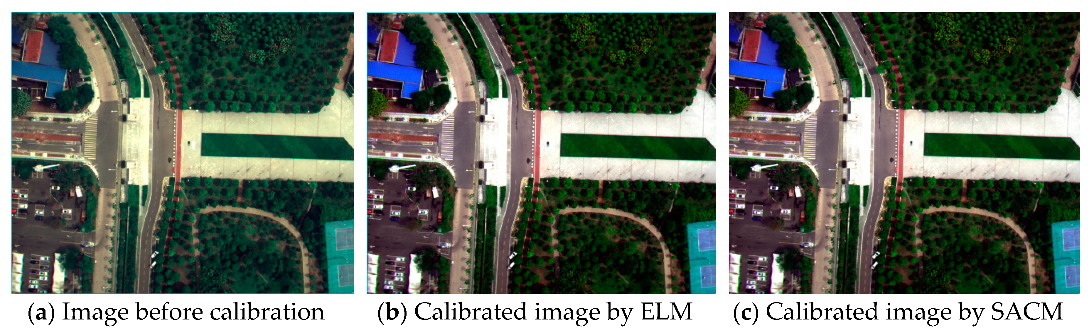
Figure 8 shows the images before and after radiometric calibration by using ELM and SACM, and the calibration coefficients of each band are shown in Table 5. Compare these three images, both of the two methods can improve the image quality if looking at the visual outcome. The brightness level of images in Figure 8b,c are obviously higher than that in Figure 8a, and it can be seen from the comparison results of the three images, there is obvious aberration in the blue and green bands before calibration, thus resulting in the image having a yellowish color. After radiometric calibration, this phenomenon can be eliminated effectively by both two methods.
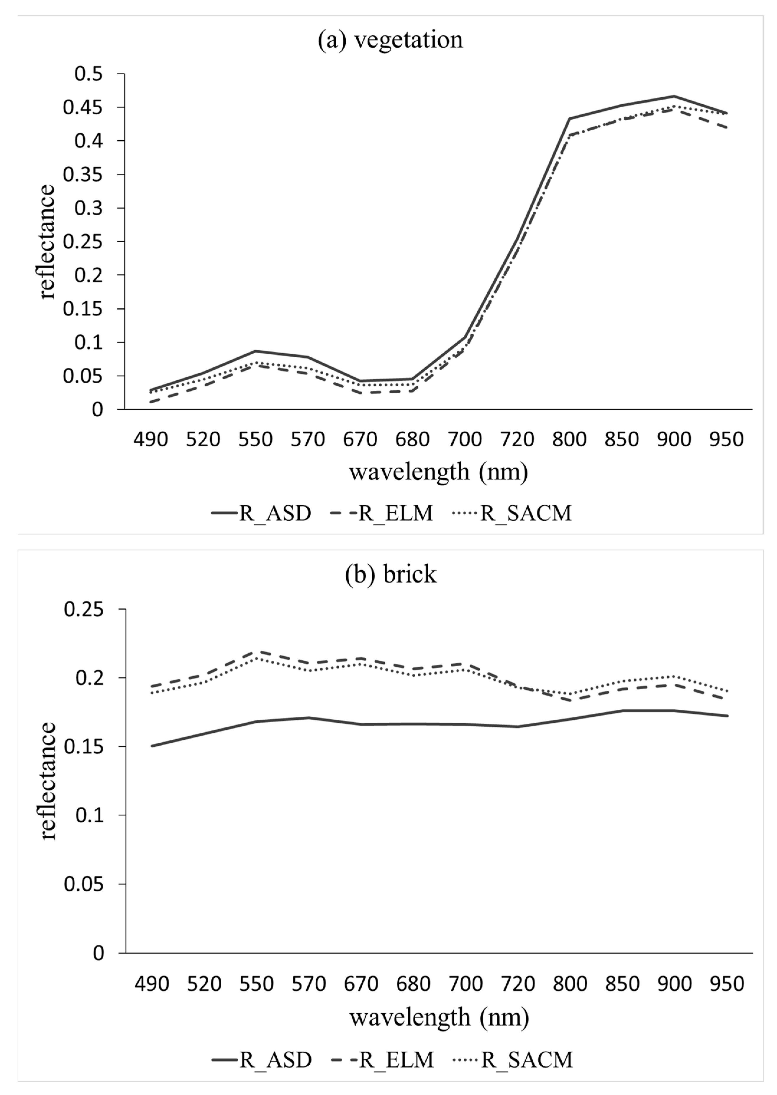
The precision of ELM and SACM were evaluated by comparing reference reflectance collected by spectroradiometer at ground level for the validation samples, and some examples were shown in Figure 9. For these samples, reflectance derived from UAV image using two radiometric calibration methods behaved similar and close to ground-measured reflectance. And it easy to find that the absolute error of each band is within 0.05 for all ground targets. By comparing the results of the two methods, the reflectance obtained by SACM is closer to the ground-measured reflectance than that obtained by ELM in most bands, especially in the visible bands.
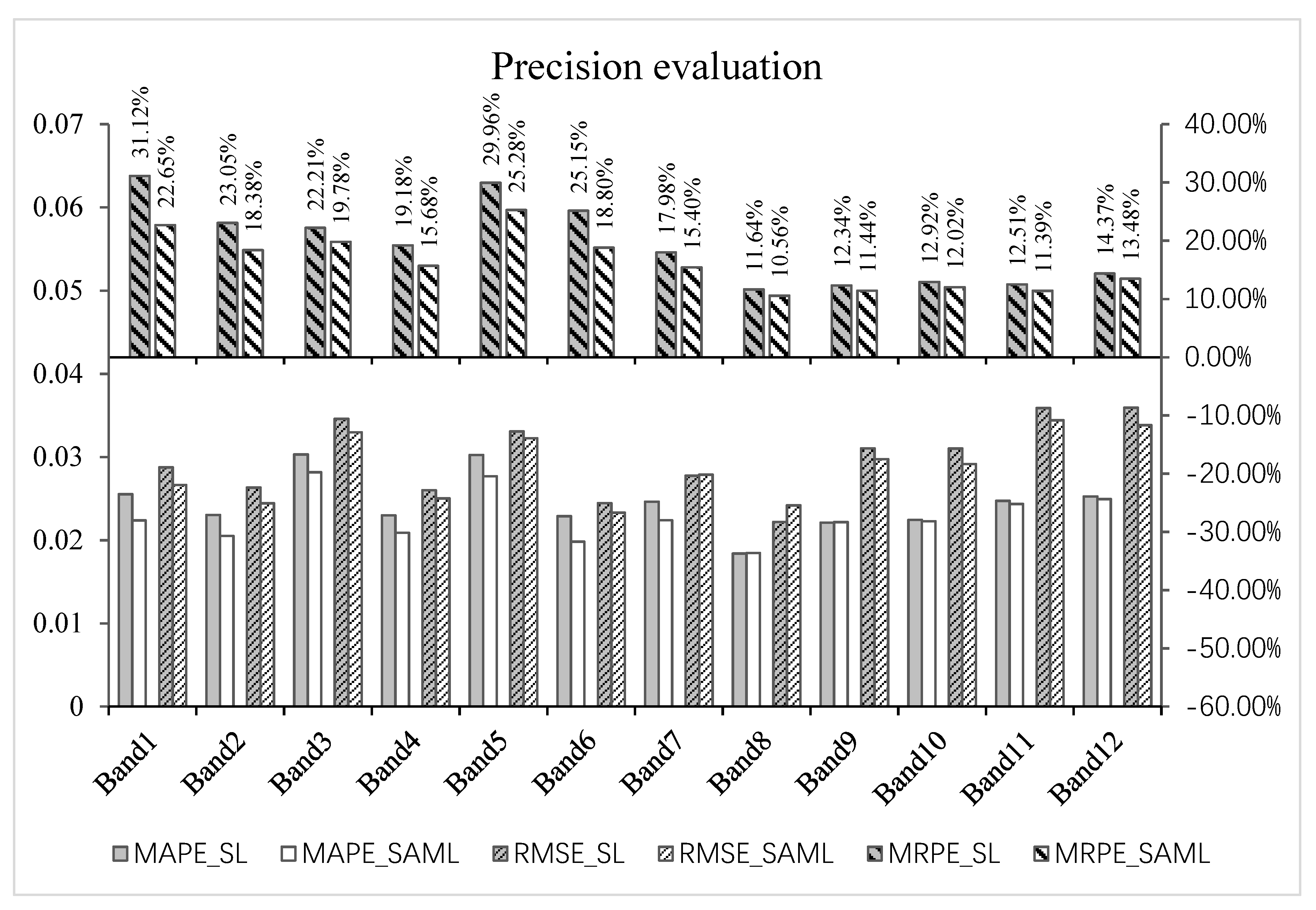
In order to evaluate the advantages and disadvantages of the two methods, the precision results of all the verified samples were statistically analyzed, and the Mean Absolute Error (MAE), Mean Relative Percent Error (MRPE) and Root Mean Square Error (RMSE) were used for evaluation. The equations of evaluation indicators are shown in Table 6, and the results are shown in Figure 10. As can be seen from Figure 10, comparing with ELM, the method proposed in this paper can improve the precision of the radiometric calibration, especially in the range of visible band, which can improve the precision obviously, with the improvement range of MRPE being more than 3% of each band. However, in the range of near-infrared band, SACM has a limited effect on the improvement of accuracy, and the precision of MRPE is basically within 1%. The precision of MAE behaved similar to that of MRPE, with obvious improvement in the visible range and limited improvement in the near-infrared band. Except bands with central wavelength of 700 nm and 720 nm, the RMSE of SACM in other bands is smaller than that of ELM, indicating that the overall precision has been improved. The results of MAE, MRPE and RMSE show that the SACM, which was proposed in this paper can realize the radiometric calibration of UAV remote sensing, and has certain advantages in radiometric calibration precision compared with the ELM.
In the formulas, R c a l , i represents the reflectance derived by ELM or SACM, R c a l , i represents the reflectance obtained by spectroradiometer, and n represents the number of samples.
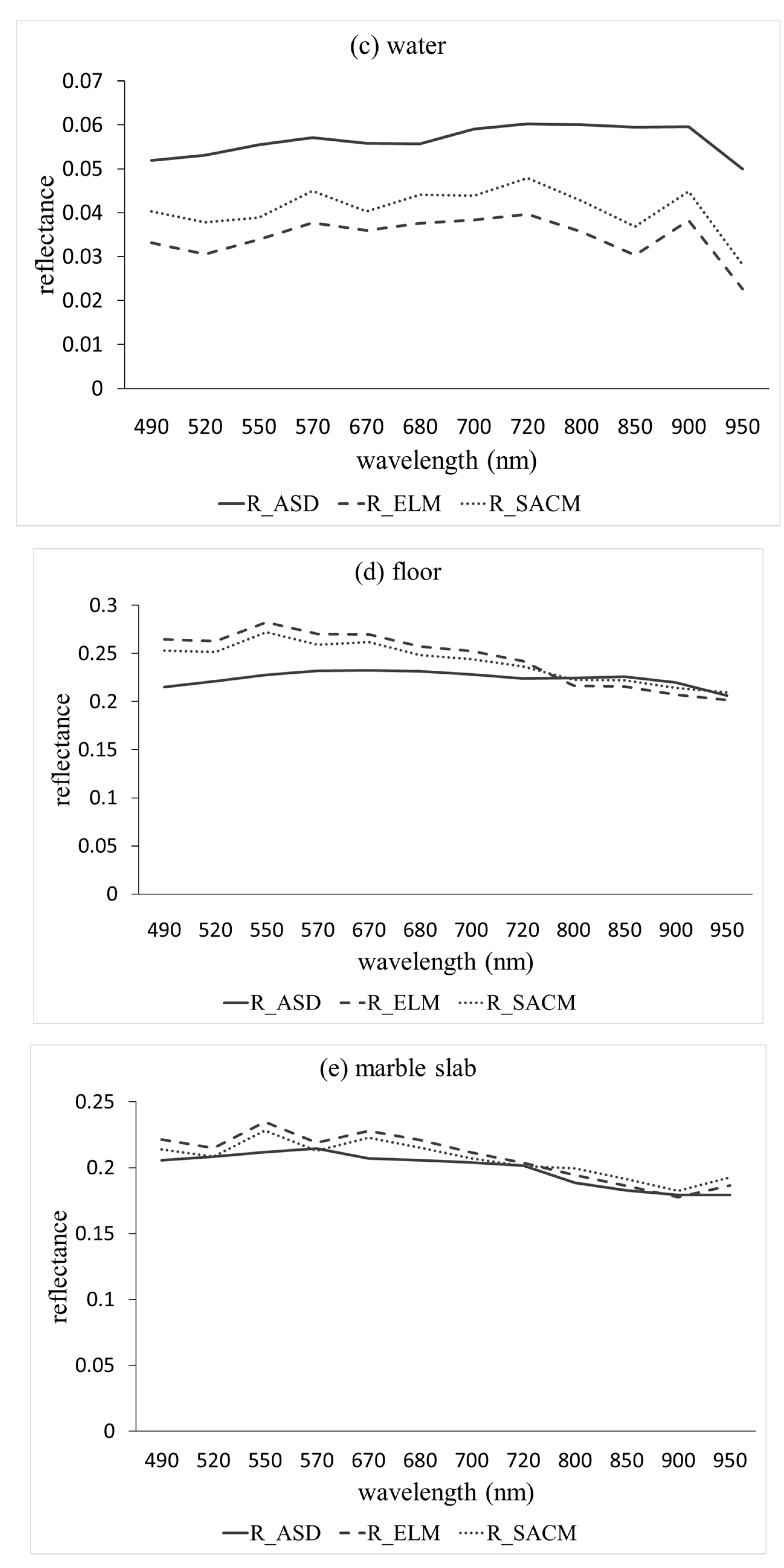
In order to further analyze the applicability of the SACM, separate experiments were conducted on different spectral constraint targets, and MAE, MRPE, and RMSE were used to verify the precision of samples, the results are shown in Figure 11, and the average errors of all bands is shown in Table 7. It can be seen in Figure 11a–c and Table 7, the radiometric calibration precision of the ELM and SACM behave similar. The calibration precision of SACM is slightly better than that of ELM in some bands, while slightly lower in other bands, and the average error of the two methods are basically consistent. However, when using vegetation for constraint modeling, SACM has great advantages in calibration precision, as shown in Figure 11d and Table 7. The average error of this method is about 5% higher than that of the ELM, and for each band, the MRPE of this method is smaller than that of the ELM. Besides, except the 8th band, the MAE and RMSE of other bands are better than that of the ELM. This result seems to show that in practical applications, the use of vegetation constraint modeling will be conducive to improve the precision of radiation calibration, and it also shows that the method proposed in this paper is more suitable for multi-vegetation coverage areas.

5. Discussion

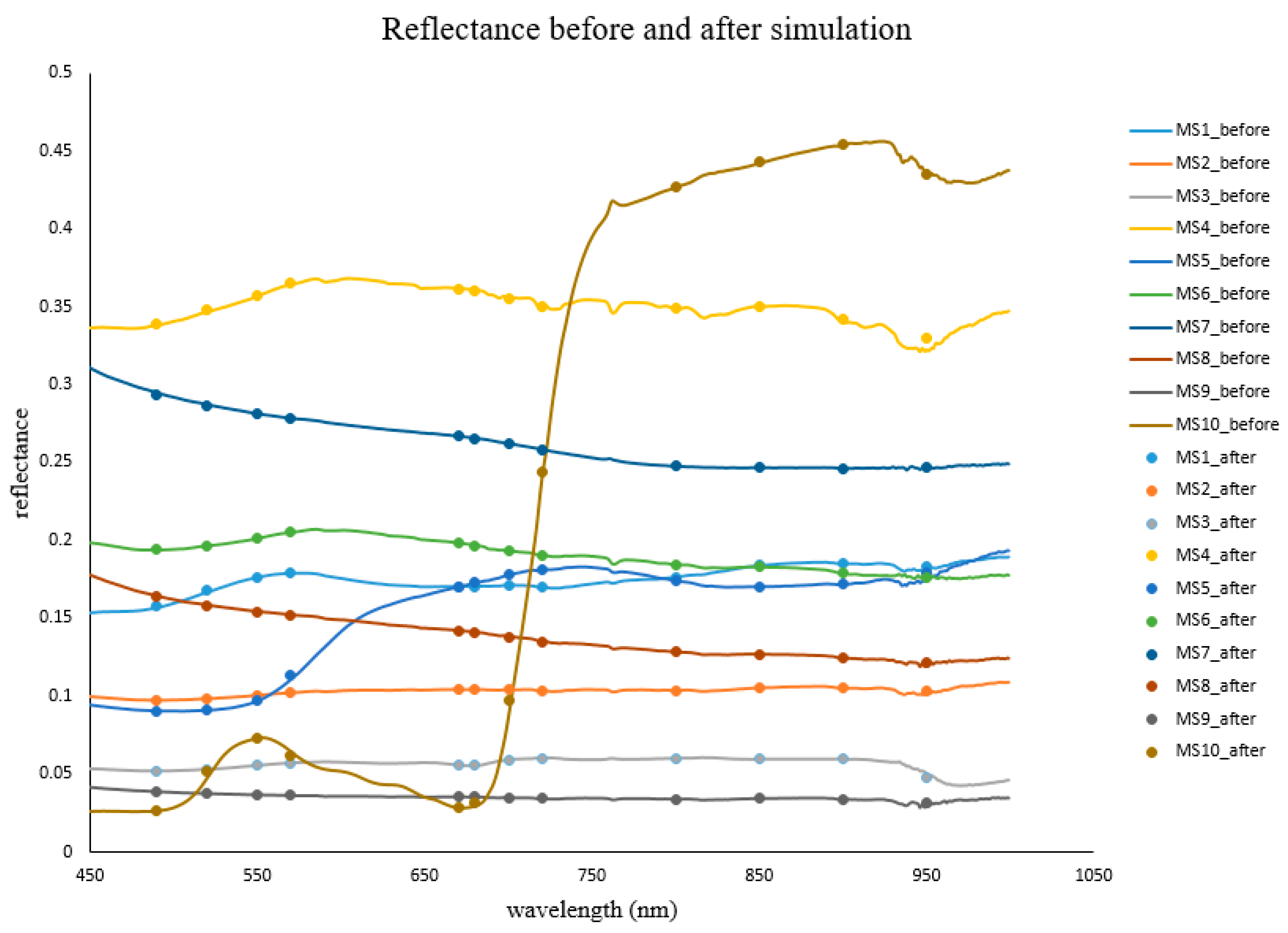
The spectral angle constraint method proposed in this paper is different from other remote sensing radiometric calibration methods of UAV. It makes full use of the spectral information of ground targets, so that the radiometric calibration process is no longer an independent calibration between each band, but combines the information of all bands to calibrate, which improves the precision of radiometric calibration. With the increase of spectral bands, the information between spectral bands will also increase. This method can make full use of the information of all bands, so for hyperspectral images, the method can provide more information in radiometric calibration, which is more conducive to improving the accuracy of radiation calibration. According to the results of separate experiments on different spectral constraint targets, the use of vegetation constraint modeling can greatly improve the precision of radiation calibration, while the results of other targets constraint modeling show that the precision of two methods is basically consistent. As can be seen from Figure 7, the form of vegetation spectral curve fluctuates greatly, while that of other ground targets is relatively flat. By using the standard deviation (STD) to evaluate the flatness of the spectral curve shape. The smaller the standard deviation is, the flatter the spectral curve of the ground object is. As can be seen from Table 8, with the increase of the standard deviation, the better the effect of using this target for constraint modeling is. Thus, it can be speculated that the ground targets with obvious fluctuation in the reflectance curves have a better effect of radiometric calibration using SACM.
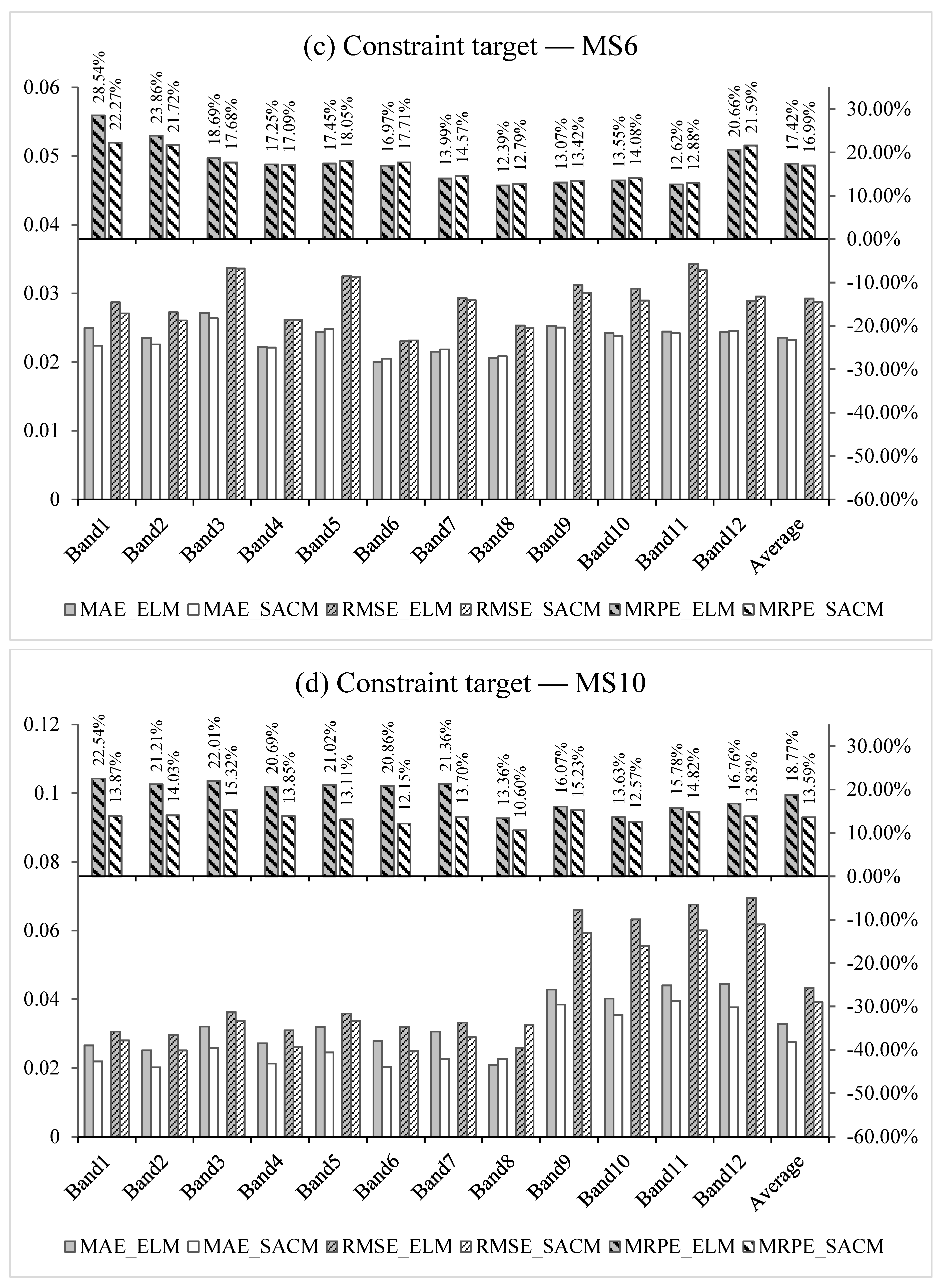
From the method in this paper, the essence is to establish a connection between the data of other bands and the target band according to Formula (10), and then generate constraint data according to Formula (11), so as to increase the amount of data used for the least squares solution. As shown in Figure 12, when the method of this paper is adopted, the number of data originally used for least squares solution increases from several to dozens. It can be found from Figure 12 that the constraint modeling is carried out by using ground targets with obvious fluctuation of spectral curves, can expand the range of modeling data. In the Figure 12a–c, it can be seen that, after the constraint, the essence is to interpolate the original sample points, which results in no improvement of calibration precision. While in Figure 12d, after vegetation constraints, the range of modeling data is not only interpolated within the original range of sample points, but also stretched, which expands the applicability of the model, and finally improves the radiation calibration precision after the constraint.
The above results show that use vegetation for constraint modeling work better than others. For many vegetation area, we can easily obtain the vegetation reflectance spectra. However, for non-vegetation-covered areas, to get vegetation reflectance spectra is difficult, and the calibration accuracy of the method in this paper is basically the same as that of the empirical linear method, but the calibration process is too complex, which restricted the application of this method, so in these areas the empirical linear method may be used for the calibration. Therefore, the method proposed in this paper is more applicable to areas with multiple vegetation coverage. For agricultural remote sensing, the method in this paper may be of great value because it focuses on crops. Therefore, the method proposed in this paper can improve the accuracy of radiometric calibration in agricultural remote sensing, thus affecting the application of agricultural remote sensing. In order to verify this conjecture, the agricultural data of EZhou was used for the experiment. Firstly, the surface reflectance data and LAI data were used to build the inversion model according to the vegetation index method [35,36,37]. Then, the UAV image was calibrated by the empirical linear method and the spectral Angle constraint method respectively, and the calibrated images were used to verify the inversion accuracy of the model. LAI images obtained by the two methods are shown in 
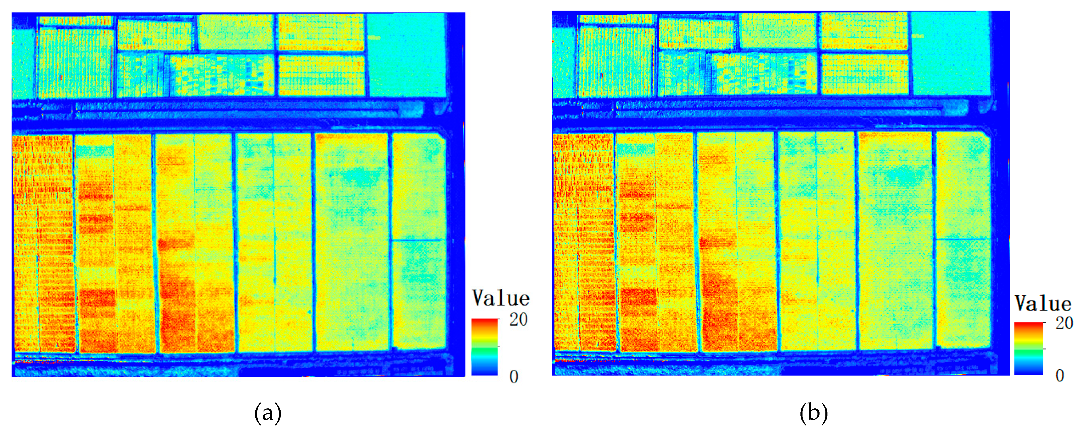
Figure 13, and their inversion accuracy is represented by the relative error of verification points (as shown in Figure 14).
As can be seen from the inversion results in Figure 14, the precision of image data after radiometric calibration with SACM in inversion LAI has been improved to a certain extent, and the relative accuracy of most verification points has been improved, with the average accuracy increased from 27% to 22%. Additionally, the standard deviation of the ELM is 0.1655, while that of the SACM is 0.1498. It can be seen from the results of standard deviation that after calibration by SACM, the precision of inversion can be improved and the results of inversion can be more stable and reliable. The above experiments also confirmed that the method proposed in this paper can be more widely used in agricultural remote sensing.

6. Conclusions

The spectral angle constraint method proposed in this paper, by introducing the spectral angle constraint condition, makes full use of the information of each band of the multi-spectral image, and considers the spectral regulation of the ground targets, so that the radiometric calibration process, which was originally solved independently for each band, can be solved as a whole. Through the research of this paper, it is shown that applying the spectral regulation of ground targets to the radiometric calibration process of UAV image can improve the accuracy of radiometric calibration. Additionally, the effect of different ground targets by using SACM show great difference. When vegetation is used for constraint modeling, the accuracy of radiation calibration can be greatly improved, while other ground targets are used for constraint modeling, the calibration accuracy of ELM and SACM is basically the same. Therefore, the method in this paper will have a great application prospect when it focuses on the reflectance information of vegetation, and its application effect in agricultural remote sensing will be very significant.

Author Contributions

All authors have made significant contributions to this manuscript. S.F. and Y.G. conceived of the research ideas. Y.G. and K.X. designed the experiment in detail and provided the majority of the writing of this paper. Z.L. and K.W. provided data and data acquisition capacity. K.X. and K.W. conducted data processing and analysis and contributed to making the figures and tables in this paper. W.F. provides advice on key technologies and provided comments and suggestions for the manuscript.

Funding

This research was supported by National Key R&D Program of China (2016YFD0101105), Civil Space Technology Pre Research Project of the thirteenth Five-Year Plan (Radiation Calibration Method for Remote Sensing Images Based on Analysis of Terrain Heterogeneity), Fundamental Research Funds for the Central Universities (2042017kf0236), and National 863 Project of China (2013AA102401).

Acknowledgments

We acknowledge the support and the use of the facilities and equipment provided by the School of Remote Sensing and Information Engineering, Wuhan University, China.

Conflicts of Interest

The authors declare no conflict of interest.

References

  1. Merino, L.; Caballero, F.; Martínez-De-Dios, J.R.; Maza, I.; Ollero, A. An Unmanned Aircraft System for Automatic Forest Fire Monitoring and Measurement. J. Intell. Robot. Syst. 2012, 65, 533–548. [Google Scholar] [CrossRef]
  2. Casbeer, D.W.; Kingston, D.B.; Beard, R.W.; Mclain, T.W. Cooperative forest fire surveillance using a team of small unmanned air vehicles. Int. J. Syst. Sci. 2006, 37, 351–360. [Google Scholar] [CrossRef]
  3. Barnard, J.A. The use of unmanned aircraft in oil, gas and mineral E+P activities. SEG Tech. Progr. Expand. Abstr. 2008, 27, 1132–1136. [Google Scholar]
  4. Spiess, T.; Bange, J.; Buschmann, M.; Vörsmann, P. First application of the meteorological Mini-UAV ‘M2AV’. Meteorol. Z. 2007, 16, 159–169. [Google Scholar] [CrossRef]
  5. Martin, S.; Bange, J.; Beyrich, F. Meteorological profiling of the lower troposphere using the research UAV “M2AV Carolo”. Atmos. Meas. Tech. 2011, 3, 705–716. [Google Scholar] [CrossRef]
  6. Hunt, E.R.; Hively, W.D.; Fujikawa, S.; Linden, D.; Daughtry, C.S.; McCarty, G. Acquisition of NIR-Green-Blue Digital Photographs from Unmanned Aircraft for Crop Monitoring. Remote Sens. 2010, 2, 290–305. [Google Scholar] [CrossRef] [Green Version]
  7. Xiang, H.; Lei, T. Development of a low-cost agricultural remote sensingsystem based on an autonomous unmanned aerial vehicle (UAV). Biosyst. Eng. 2011, 108, 174–190. [Google Scholar] [CrossRef]
  8. Wang, C.; Price, K.P.; Merwe, D.V.D.; Nan, A.; Wang, H. Modeling Above-Ground Biomass in Tallgrass Prairie Using Ultra-High Spatial Resolution sUAS Imagery. Photogramm. Eng. Remote Sens. 2015, 80, 1151–1159. [Google Scholar] [CrossRef]
  9. Rango, A.; Laliberte, A.; Herrick, J.E.; Winters, C.; Havstad, K.; Steele, C.; Browning, D. Unmanned aerial vehicle-based remote sensing for rangeland assessment, monitoring, and management. Chin. Hydraul. Pneum. 2009, 3, 11–15. [Google Scholar]
  10. Kelcey, J.; Lucieer, A. Sensor correction and Radiometric calibration of a 6-band multispectral imaging sensor for UAV remote sensing. ISPRS Int. Arch. Photogramm. Remote Sens. Spat. Inf. Sci. 2012, 39-B1, 393–398. [Google Scholar] [CrossRef]
  11. Yang, G.; Liu, J.; Zhao, C.; Li, Z.; Huang, Y.; Yu, H.; Xu, B.; Yang, X.; Zhu, D.; Zhang, X. Unmanned Aerial Vehicle Remote Sensing for Field-Based Crop Phenotyping: Current Status and Perspectives. Front. Plant Sci. 2017, 8, 1111. [Google Scholar] [CrossRef]
  12. Hadjimitsis, D.G.; Clayton, C.R.I.; Hope, V.S. An assessment of the effectiveness of atmospheric correction algorithms through the remote sensing of some reservoirs. Int. J. Remote Sens. 2004, 25, 3651–3674. [Google Scholar] [CrossRef]
  13. Iqbal, F.; Lucieer, A.; Barry, K. Simplified radiometric calibration for UAS-mounted multispectral sensor. Eur. J. Remote Sens. 2018, 51, 301–313. [Google Scholar] [CrossRef]
  14. Pozo, S.D.; Rodríguez-Gonzálvez, P.; Hernández-López, D.; Felipe-García, B. Vicarious Radiometric Calibration of Multispectral Camera on Board Unmanned Aerial System. Remote Sens. 2014, 6, 1918–1937. [Google Scholar] [CrossRef]
  15. Lei, D.; Hao, X.; Mao, Z.; Yan, Y.; Jie, S.; Zhang, A. A Subband Radiometric Calibration Method for UAV-Based Multispectral Remote Sensing. IEEE J. Sel. Top. Appl. Earth Obs. Remote Sens. 2018, 11, 2869–2880. [Google Scholar]
  16. Mafanya, M.; Tsele, P.; Botai, J.O.; Manyama, P.; Chirima, G.J.; Monate, T. Radiometric calibration framework for ultra-high-resolution UAV-derived orthomosaics for large-scale mapping of invasive alien plants in semi-arid woodlands: Harrisia pomanensis as a case study. Int. J. Remote Sens. 2018, 39, 5119–5140. [Google Scholar] [CrossRef]
  17. Moran, M.S.; Bryant, R.; Thome, K.; Ni, W.; Nouvellon, Y.; Gonzalez-Dugo, M.P.; Qi, J.; Clarke, T.R. A refined empirical line approach for reflectance factor retrieval from Landsat-5 TM and Landsat-7 ETM+. Remote Sens. Environ. 2001, 78, 71–82. [Google Scholar] [CrossRef]
  18. Ben-Dor, E.; Kruse, F.A.; Lefkoff, A.B.; Banin, A. Comparison of three calibration techniques for utilization of GER 63- channel aircraft scanner data of Makhtesh Ramon, Negev, Israel. Photogramm. Eng. Remote Sens. 1994, 60, 1339–1354. [Google Scholar]
  19. Dwyer, J.L.; Kruse, F.A.; Lefkoff, A.B. Effects of empirical versus model-based reflectance calibration on automated analysis of imaging spectrometer data: A case study from the Drum Mountains, Utah. Photogramm. Eng. Remote Sens. 1995, 61, 1247–1254. [Google Scholar]
  20. Laliberte, A.S.; Goforth, M.A.; Steele, C.M.; Rango, A. Multispectral Remote Sensing from Unmanned Aircraft: Image Processing Workflows and Applications for Rangeland Environments. Remote Sens. 2011, 3, 2529–2551. [Google Scholar] [CrossRef] [Green Version]
  21. Miura, T.; Huete, A.R. Performance of three reflectance calibration methods for airborne hyperspectral spectrometer data. Sensors 2009, 9, 794–813. [Google Scholar] [CrossRef]
  22. Karpouzli, E.; Malthus, T. The empirical line method for the atmospheric correction of IKONOS imagery. Int. J. Remote Sens. 2003, 24, 1143–1150. [Google Scholar] [CrossRef]
  23. Smith, G.; Milton, E. The use of the empirical line method to calibrate remotely sensed data to reflectance. Int. J. Remote. Sens. 1999, 20, 2653–2662. [Google Scholar] [CrossRef]
  24. Wang, C.; Myint, S.W. A Simplified Empirical Line Method of Radiometric Calibration for Small Unmanned Aircraft Systems-Based Remote Sensing. IEEE J. Sel. Top. Appl. Earth Obs. Remote Sens. 2015, 8, 1876–1885. [Google Scholar] [CrossRef]
  25. Cuirolo, A.; Plata, K.; Rosato, A.E. Empirical line calibration of WorldView-2 satellite imagery to reflectance data: Using quadratic prediction equations. Remote Sens. Lett. 2012, 3, 521–530. [Google Scholar]
  26. Stow, D.; Hope, A.; Nguyen, A.T.; Phinn, S.; Benkelman, C.A. Monitoring detailed land surface changes using a multispectral digital camera system. IEEE Trans. Geosci. Remote Sens. 1996, 34, 1191–1203. [Google Scholar] [CrossRef]
  27. Sims, D.A.; Gamon, J.A. Relationships between leaf pigment content and spectral reflectance across a wide range of species, leaf structures and developmental stages. Remote Sens. Environ. 2002, 81, 337–354. [Google Scholar] [CrossRef]
  28. Zhang, F.; Tiyip, T.; Ding, J.; Sawut, M.; Tashpolat, N.; Kung, H.; Han, G.; Gui, D. Spectral reflectance properties of major objects in desert oasis: A case study of the Weigan—Kuqa river delta oasis in Xinjiang, China. Environ. Monit. Assess. 2012, 184, 5105–5119. [Google Scholar] [CrossRef]
  29. Gao, L.; Yang, B.; Du, Q.; Zhang, B. Adjusted Spectral Matched Filter for Target Detection in Hyperspectral Imagery. Remote Sens. 2015, 7, 6611–6634. [Google Scholar] [CrossRef] [Green Version]
  30. Kruse, F.A.; Boardman, J.W.; Huntington, J.F. Comparison of Airborne Hyperspectral Data and EO-1 Hyperion for Mineral Mapping. IEEE Trans. Geosci. Remote Sens. 2003, 41, 1388–1400. [Google Scholar] [CrossRef]
  31. Schmidt, F.; Legendre, M.; Mouëlic, S.L. Minerals detection for hyperspectral images using adapted linear unmixing: LinMin. Icarus 2014, 237, 61–74. [Google Scholar] [CrossRef] [Green Version]
  32. Tarabalka, Y.; Benediktsson, J.A.; Chanussot, J. Spectral—Spatial Classification of Hyperspectral Imagery Based on Partitional Clustering Techniques. IEEE Trans. Geosci. Remote Sens. 2009, 47, 2973–2987. [Google Scholar] [CrossRef]
  33. van der Meer, F. The effectiveness of spectral similarity measures for the analysis of hyperspectral imagery. Int. J. Appl. Earth Obs. Geoinf. 2006, 8, 3–17. [Google Scholar] [CrossRef]
  34. Sweet, J.N. The spectral similarity scale and its application to the classification of hyperspectral remote sensing data. In IEEE Workshop on Advances in Techniques for Analysis of Remotely Sensed Data; IEEE: Piscataway, NJ, USA, 2004. [Google Scholar]
  35. Cammarano, D.; Fitzgerald, G.J.; Casa, R.; Basso, B. Assessing the Robustness of Vegetation Indices to Estimate Wheat N in Mediterranean Environments. Remote Sens. 2014, 6, 2827–2844. [Google Scholar] [CrossRef] [Green Version]
  36. Fang, S.; Yuan, L.; Qi, L.; Liu, X. Leaf Area Index Estimation Using Time-Series MODIS Data in Different Types of Vegetation. J. Indian Soc. Remote 2014, 42, 733–743. [Google Scholar] [CrossRef]
  37. Verrelst, J.; Rivera, J.P.; Veroustraete, F.; Muñoz-Marí, J.; Clevers, J.G.P.W.; Camps-Valls, G.; Moreno, J. Experimental Sentinel-2 LAI estimation using parametric, non-parametric and physical retrieval methods —A comparison. ISPRS J. Photogramm. Remote Sens. 2015, 108, 260–272. [Google Scholar] [CrossRef]
Figure 1. Study area in Wuhan city, China.
Remotesensing 11 01291 g001
Figure 2. Mini-MCA12 multispectral camera.
Remotesensing 11 01291 g002
Figure 3. The spectral response of filters.
Remotesensing 11 01291 g003
Figure 4. Spreading Wings S1000.
Remotesensing 11 01291 g004
Figure 5. ASD FieldSpec4 Standard-Res.
Remotesensing 11 01291 g005
Figure 6. UAV image of the control and check surfaces.
Remotesensing 11 01291 g006
Figure 7. Reflectance before and after simulation.
Remotesensing 11 01291 g007
Figure 8. The images of the study area before and after calibration.
Remotesensing 11 01291 g008
Figure 9. Comparison of ground-measured reflectance and reflectance derived from radiometric calibrated image using ELM and SACM in different bands for samples of (a) vegetation, (b) brick, (c) water, (d) floor, and (e) marble slab. R_ASD represents the relectance obtain by spectroradiometer, R_ELM and R_SACM represent the refectance derived by ELM and SACM.
Remotesensing 11 01291 g009aRemotesensing 11 01291 g009b
Figure 10. Precision evaluation of ELM and SACM.
Remotesensing 11 01291 g010
Figure 11. The MAE, MRPE and RMSE of the radiometric calibration using ELM and SACM for different constraint targets of (a) MS1 (brick), (b) MS3 (water), (c) MS6 (floor) and (d) MS10 (vegetation).
Remotesensing 11 01291 g011aRemotesensing 11 01291 g011b
Figure 12. Data generated after constraint modeling of different ground targets. (ad) represent the results of constraint modeling with MS1 (brick), MS3 (water), MS6 (floor) and MS10 (vegetation) respectively.
Remotesensing 11 01291 g012
Figure 13. The LAI inversion results of calibrated images. (a) s the calirated image obtained by ELM and (b) is the calibrated image obtained by SACM.
Remotesensing 11 01291 g013
Figure 14. The LAI inversion accuracy of the two methods.
Remotesensing 11 01291 g014
Table 1. Specifications of Mini-MCA.
ParameterValue
Number of channels12
Weight1300 g
Geometric resolution1280 × 1024 pixels
Radiometric resolutionRAW 8 bit/RAW 10 bit/DCM 10 bit
Speed1.3 frames/s
Dimensions6.66 mm × 5.32 mm
Pixel size5.2 µm
Focal length9.6 mm
Table 2. Characteristics of the twelve channels.
Channel NumberCentral Wavelength(nm)FWHMBand Width Range (nm)
149010470–510
252010500–540
355010530–570
457010550–590
567010650–690
668010660–700
770010680–720
872010700–740
980010780–820
1085010830–870
1190020860–940
1295040870–1030
Table 3. Characteristics of the UAV.
ParameterValue
Takeoff weight6 kg~11 kg
Total weight4.2 kg
Estimated flight time15 min (@9.5 kg takeoff weight)
Power battery10,000 mAh~20,000 mAh
Table 4. Characteristics of the spectroradiometer.
ParameterValue
TypeFieldSpec4 Standard-Res
Band width range (nm)350–2500
Spectral sampling interval1.4 nm(350–1000 nm); 2 nm(1001–2500 nm)
Spectral resolution3 nm@700 nm; 10 nm@1400, 2100 nm
Table 5. The calibration coefficients of each band.
ELM_aELM_bSACM_aSACM_b
Band 11.44 * 10−3−4.29 * 10−21.31 * 10−3−2.55 * 10−2
Band 21.79 * 10−3−7.19 * 10−21.62 * 10−3−5.12 * 10−2
Band 31.35 * 10−3−4.14 * 10−21.24 * 10−3−2.58 * 10−2
Band 41.62 * 10−3−3.74 * 10−21.46 * 10−3−1.89 * 10−2
Band 51.32 * 10−3−3.96 * 10−21.23 * 10−3−2.64 * 10−2
Band 61.51 * 10−3−3.82 * 10−21.38 * 10−3−2.16 * 10−2
Band 71.81 * 10−3−7.94 * 10−21.65 * 10−3−5.84 * 10−2
Band 82.44 * 10−3−4.16 * 10−22.21 * 10−3−2.01 * 10−2
Band 92.23 * 10−3−5.28 * 10−22.15 * 10−3−4.26 * 10−2
Band 102.43 * 10−3−1.11 * 10−22.55 * 10−3−1.56 * 10−2
Band 113.44 * 10−3−1.73 * 10−23.63 * 10−3−2.30 * 10−2
Band 128.33 * 10−3−7.85 * 10−29.03 * 10−3−9.46 * 10−2
Table 6. Error equation.
ErrorAbbreviationEquation
Mean Absolute ErrorMAE 1 n i = 1 n | R c a l , i R A S D , i |
Mean Relative Percent ErrorMRPE 1 n i = 1 n | 100 × R c a l , i R A S D , i R A S D , i |
Root Mean Square ErrorRMSE i = 1 n ( R c a l , i R A S D , i ) 2 n
Table 7. The average error of MAE, MRPE and RMSE for different constraint targets.
Constraint TargetMRPEMAERMSE
Vegetation
ELM18.77%0.03280.0434
SACM13.59%0.02750.0391
Water
ELM19.75%0.02880.0327
SACM19.72%0.02880.0327
Brick
ELM21.34%0.02660.0298
SACM21.08%0.02640.0298
Floor
ELM17.42%0.02360.0293
SACM16.99%0.02320.0287
Table 8. The standard deviation and precision improve effect.
Constraint TargetSTDDMRPEDMAEDRMSE
Water0.00340.03%00
Brick0.00810.26%0.00020
Floor0.00900.43%0.00040.0006
Vegetation0.18845.18%0.00530.0043
DMRPE, DMAE and DRMSE respectively represent the difference between the two methods of MRPE, MAE and RMSE.

